This page intentionally left blank
4
CHAPTER
ANIMATION
Animation is what ultimately breathes life into 3D graphics. While still images can be
nice as such, most applications involve objects moving and interacting with each other
and the user, or scenes in some other way changing over time. This chapter introduces
basic, commonly used animation concepts that we will encounter when we discuss the
M3G animation functionality later in the book.
4.1 KEYFRAME ANIMATION
Keyframe animation is perhaps the most common way of describing predefined motions
in computer graphics. The term originates from cartoons, where the senior animator
would first draw the most important “key” frames describing the main poses within
an animation sequence. The in-between frames or “tweens” could then be filled in to
complete the animation, based on those defining features. This allowed the valuable time
of the senior animator to be focused on the important parts, whereas the work of drawing
the intermediate frames could be divided among the junior colleagues.
In computer animation today, a human animator still defines the keyframes, but the
data in between is interpolated by the computer. An example of keyframe interpolation
is shown in Figure 4.1. The keyframes are values that the animated property has at
specific points in time, and the computer applies an interpolation function to these
data points to produce the intermediate values. The data itself can be anything from
105
106 ANIMATION CHAPTER 4
value
time
Figure 4.1: Keyframe values (points) and interpolated data (curve).
positions and orientations to color and lighting parameters, as long as it can be
represented numerically to the computer.
Expressing this mathematically, we have the set of N keyframes K = (k
0

, k
1
, , k
N−1
)
and an interpolation function f. The value of the animated property can then be evalu-
ated at any time t by evaluating f (K, t); we can also say that we sample the animated value
at different times t. Using different functions f, we can vary the characteristics of the
interpolated data, as well as the computational complexity of evaluating the function.
The main benefit of keyframe animation today is perhaps not the time saved in producing
the animation, but the memory saved by the keyframe representation. Data need only be
stored at the keyframe locations, and since much of the animation data required can be
produced from fairly sparse keyframes, keyframe animation is much more space-efficient
than storing the data for each frame. A related benefit is that the keyframe rate need not
be tied to the display rate; once you have your keyframe sequence, you can play it back at
any rate, speeding up or slowing down as necessary.
4.1.1 INTERPOLATION
In practice, interpolation is usually implemented in a piecewise manner: each interpolated
segment, separated by two adjacent keyframes, is computed on its own, and the slope
or curvature of the adjacent segments has no effect on the result. In some schemes, the
interpolation parameters depend on the keyframes of the adjacent segments as well, but
once those parameters are known, each segment is still interpolated as a separate entity.
Interpolating an entire keyframe sequence amounts to identifying the segment we are
interested in, by finding the keyframes surrounding our sampling time t, and computing
the interpolated value for that segment only. Let us call the values of our chosen keyframes
simply a and b. Those will be the desired values at the beginning and end of the segment,
SECTION 4.1 KEYFRAME ANIMATION 107
respectively. Let us also define a new interpolation parameter s, derived from time t,to
give our position within the segment: the value of s shall be 0 at keyframe a and increase
linearly to 1 at keyframe b. Armed with this information, we can begin looking for differ-

entwaystomovefroma to b.
The simplest way to interpolate keyframes is the step function, which does not interpolate
at all:
f
step
(s) = a.
(4.1)
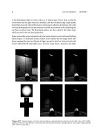
Instead, as show n in Figure 4.2, the interpolated value always remains at that of the
previous keyframe. This is very easy from a computational perspective, but as seen in
the figure, it produces a discontinuous result that is ill-suited to animating most aspects
of a visual scene—for example, a character jumping from one place to another is not what
we typically expect of animation. The step function can still have its uses: switching lig ht
sources on and off at preprogrammed times is one intuitive application.
Going toward smoother motion, we need to take into account more than one keyframe.
Using both keyframes, we can linearly interpolate, or lerp, between them:
f
lerp
(s) = (1 − s)a + sb
(4.2)
= a + s(b − a). (4.3)
value
time
Figure 4.2: Step interpolation.
108 ANIMATION CHAPTER 4
value
time
Figure 4.3: Linear interpolation, or lerp.
As we can see in Figure 4.3, ler p actually connects the keyframes without sudden jumps.
However, it is immediately obvious that the result is not smooth: the direction of our inter-
polated line changes abruptly at each keyframe, and the visual effect is very similar. This,

again, defies any expectations of physically based motion, where some manner of inertia
is to be expected. Lerping is still computationally very cheap, which makes it well suited
to ramping things such as light levels up and down at various speeds, and it can be used to
approximate nonlinear motion by adding more keyframes. Of course, any purely linear
motion at constant speed is a natural application, but such motions are quite uncommon
in practice—consider, for example, city traffic during rush hour, or the individual limbs
and joints of a walking human.
For more life-like animation, we need a function that can provide some degree of ease-in
and ease-out: instead of jumping into and out of motion, short periods of acceleration
and deceleration make the animation appear much more natural. Also, since much of
the animation in computer graphics is not linear, being able to represent curved motion
is another feature in the w ish list. It would seem that changing the linear segments of
Figure 4.3 into curved ones would solve both problems, and indeed it does—in a number
of different flavors. There are many different formulations for producing curves, each
with its individual characteristics that make it better suited for some particular tasks and
less well for others. In the following, we will only cover what is relevant to using and
understanding M3G in the later chapters of this book.
SECTION 4.1 KEYFRAME ANIMATION 109
The curves commonly used in computer graphics are parametric cubic curves,whichoffer
a good balance between the amount of control, computational efficiency, and ease of use
[FvFH90]. Each interpolated curve segment is a separate polynomial function of s that
connects the two keyframes a and b. Depending on the type of curve, the actual polyno-
mial coefficients are usually defined through more intuitive parameters, such as additional
control points or explicit tangent vectors. In this discussion, we will use a Hermite curve
[FvFH90, AMH02] to construct a Catmull-Rom spline [CR74] that smoothly interpolates
our keyframe sequence similarly to Figure 4.4.
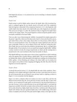
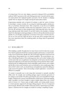
As illustrated in Figure 4.5, each Hermite curve segment is controlled by tangent vectors
at both ends in addition to the actual keyframes. If you think of interpolating the position
of an object using a Hermite curve, the tangent vectors are essentially the velocity—speed
and direction—of the object at the endpoints of the curve.

When discussing lerp, we mentioned that natural objects do not jump from one position
to another, and neither do they change velocity abruptly. For natural-looking motion,
we therefore want not only the position, but also the velocity to be continuous. There-
fore, when interpolating across multiple segments, we want to align the tangent vec-
tors between neighboring segments such that the velocity remains constant. Since our
keyframes are not necessarily spaced uniformly in time, we cannot trivially use the
same tangent vector for both segments connected to a keyframe; instead, the tangents
value
time
Figure 4.4: Curve interpolation.
110 ANIMATION CHAPTER 4
x
y
c
a9
1
b9
2
b9
1
c9
2
b
a
Figure 4.5: Two Hermite curve segments and their tangent vectors; the end tangent of each seg-
ment is reversed for clarity. In order to illustrate the tangent vectors, the coordinate system is different
from Figures 4.2 to 4.4, and time is not plotted at all. Note that the relative magnitude of tangents
b
−
and b

+
depends on keyframe timing and need not be the same; see text.
may have to be scaled to different magnitudes in order to maintain smooth velocity
[KB84, AMH02].
In order to compute the tangent vectors b

−
and b

+
using the three-keyframe sequence
(a, b, c) in Figure 4.5 so that they maintain smooth motion over keyframe b,weneed
to take into account the durations of the adjacent interpolation segments. Let us denote
the time differences between b and its adjacent keyframes by Δt
ab
and Δt
bc
. Our tangent
values will then be [KB84, AMH02]
b

−
=
Δt
ab
Δt
ab
+Δt
bc
b


(4.4)
and
b

+
=
Δt
bc
Δt
ab
+Δt
bc
b

, (4.5)
where b

is a finite central difference over keyframe b:
b

=
c − a
2
.
(4.6)
The tangents for keyframes a and c are computed in a similar manner from their adjacent
keyframes.
SECTION 4.1 KEYFRAME ANIMATION 111
Based on the equations for Hermite curve interpolation [AMH02, FvFH90, WW92]

and the tangent vectors we defined above, we can, again, express the segment between
keyframes a and b as a function of our interpolation parameter s:
f
spline
(s) = [aba

+
b

−
] M
T
[s
3
s
2
s 1]
T
, (4.7)
where M is a basis matrix of coefficients specific to a Hermite curve:
M =
⎡
⎢
⎢
⎢
⎣
2 −21 1
−33−2 −1
0010
1000

⎤
⎥
⎥
⎥
⎦
. (4.8)
As we have mentioned, there are numerous other classes of curves and splines used in
computer graphics. One type of spline commonly used in animation and modeling tools
is an extension of Catmull-Rom splines called Kochanek-Bartels splines [KB84]. They
are also known as TCB splines after the tension, continuity, and bias parameters they add
to control the shape of the curve at each keyframe. However, for the purposes of this
book, it is sufficient to know that it is possible to approximate the shape of any other
curve using Catmull-Rom curves, to an arbitrary degree, by adding more keyframes. For
further reading on other kinds of curves, again, refer to more comprehensive computer
graphics textbooks [FvFH90, AMH02, WW92].
4.1.2 QUATERNIONS
Interpolating positions and most other parameters is easy to understand: you can plot
the keyframe values on paper, draw a line or curve in between, and pick any point on
the line for an intuitive interpolated position. You can interpolate each of the x, y, and z
coordinates independently and get the correct result. Interpolating orientations, however,
is not quite as intuitive.
Most computer animation today, M3G included, uses unit quaternions to represent ori-
entation, as described in Section 2.3.1. As a quick recap, a unit quaternion is a four-vector
[xyzw] of length one where the first three imaginary components relate to an axis
of rotation and the last, real, component relates to a rotation angle.
Each and e very quaternion that we are interested in will always rest on a four-dimensional
sphere that has a radius of one. Imagine that the unit sphere of quaternions has a North
pole (at [0 0 0 1]) and a South pole (at [0 0 0 −1]). The quaternion on the
Nor th pole stands for the initial position of your object, before any rotation has been
applied to it. Each quaternion elsewhere on the surface of the sphere represents a rotation

away from the initial position. The farther you go from the North pole, the more you
rotate. Walking along the shortest path possible along the surface will rotate along the
112 ANIMATION CHAPTER 4
shortest path (and about a single axis) between two orientations. However, moving by
any number of degrees on the 4D sphere will rotate twice that number in 3D space—refer
to Equation 2.21 for the proof. Therefore, if you reach the South pole, your 3D object will
have rotated a full 360 degrees, back to where it started from; but it is important to realize
that in quaternion space, we could not be farther away from the initial position!
To interpolate along the surface of the 4D sphere, spherical linear interpolation or slerp
can be used. Assuming two unit quaternion keyframes
ˆ
a and
ˆ
b, with the interpolation arc
angle θ defined such that cos θ =
ˆ
a ·
ˆ
b, slerp is defined as:
f
slerp
(s) = slerp(s :
ˆ
a,
ˆ
b) =
ˆ
a sin((1 − s)θ) +
ˆ
b sin(sθ)

sin(θ)
. (4.9)
Each quaternion
ˆ
q has a counterpart −
ˆ
q, on exactly the opposite side of the unit sphere,
which results in exactly the same orientation. As long as you are dealing with rotations
of 180 degrees or less, you can optimize your slerp routine a bit by explicitly flipping
the signs on one of the quaternions so that they land on the same hemisphere of the 4D
unit sphere. This is what many code examples on quaternion interpolation do, and it will
work as long as all you want is to interpolate along the shortest path between two 3D
orientations. However, sometimes you may want to interpolate along the longer path, in
the opposite direction, or blend between more than two orientations, and in such a case
using the whole 4D unit sphere is required.
Also, using the proper slerp without any sign mangling, you can actually rotate by
up to 360 deg rees between two keyframes, so there is more power available to you
that way. In any case, be warned that unless you know very well what you are doing,
you will be better off using the full-blown slerp for interpolation. On the other hand,
you will also need to take greater care when exporting the animations from your tools;
some of these only return the orientation keyframes as matrices, requiring a conversion
back to quaternions, and you will need to decide between the quaternions
ˆ
q and −
ˆ
q
for each matrix. However, this small headache will enable the rest of the animation
pipeline to work correctly also when more advanced features than simple two-keyframe
interpolation are introduced.
Slerp for quaternions has the same problem as lerp for positions: you get instant changes

in angular velocity at keyframes. The solution is also similar: use curved interpolation.
The equivalent of splines for quaternions is often dubbed squad. We omit the associated
hairy math here, but for more details, refer to the paper by Shoemake [Sho87] or a graph-
ics book that treats the subject [WW92, AMH02]. Suffice it to say that squad will inter-
polate rotations like spline interpolates positions, albeit with increased computational
intensity. In practice, slerp or even lerp followed by renormalization (Equation (2.4)) is
often sufficient for purposes such as character animation, and regular spline interpola-
tion can be leveraged for most use cases. Squad can still be useful for achieving perfectly
smooth camera interpolation, for example.
SECTION 4.2 DEFORMING MESHES 113
4.2 DEFORMING MESHES
Keyframe animation is good for controlling animated objects, for example moving the
limbs of an articulated character. If we are modeling robots, rigid-body animation suffices,
and we can just render the pieces individually. To affect the motion on a more soft-bodied
character, however, we want the mesh to deform without seams or cracks. This calls for
some form of per-vertex deformation.
4.2.1 MORPHING
A straightforward way to animate a mesh is to do as the cartoonists do: define keyframes
that comprise the essential poses of an animation, then interpolate or morph between
those. A simple example is shown in Figure 4.6. The way we can do this is to define a set
of alternative vertex array definitions M
0
, M
1
, M
2
, , M
N−1
so that each M
i

represents
the vertex coordinates (and other related data, such as normals and texture coordinates)
for one keyframe. The mesh topology or list of primitives is only specified once.
To interpolate between the mesh keyframes, we can just lerp between any two of them if
the keyframes represent poses on a timeline. Better yet, we can think of our keyframes as
alternative shapes, or morph targets, that we can arbitrarily blend between:
M =

w
i
M
i
,
(4.10)
where the w
i
are weights we can freely assign to each of the morph targets. Note that using
weights outside of the [0, 1] range, it is also possible to extrapolate the predefined shapes.
An alternative formulation is to add the weighted morph targets to a base shape:
M = B +

w
i
M
i
(4.11)
This emphasizes the role of some base shape that is being modified through morphing,
but mathematically, both formulations express the same thing.
Figure 4.6: Morphing some of the vertex positions between the two base shapes on the left and the right. Note that the
number of vertices remains the same.