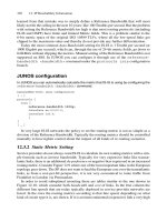
The IS-IS configuration looks alright – all interfaces are referenced. At the top there is
a pointer to an export policy which we will examine closer.
JUNOS configuration
On first sight the static-to-isis policy looks good, however once you check the inden-
tation of the terms and accept statements you will find out that the policy does not do what
the network operator wanted it to do.
hannes@Munich> show configuration policy-options
[… ]
policy-statement static-to-isis {
term reject_management {
from {
route-filter 10.0.0.0/8 orlonger;
}
then reject;
}
term static {
from protocol static;
}
then accept;
}
At first sight this policy looks good. However, once we start to compare the indenta-
tion of the then part we realize that the term static does not have a valid then state-
ment. Due to a misconfiguration, it got inserted at the wrong level in the policy. What the
standalone then accept term does is accept every unicast route in the inet.0 routing
tables and mark it for export into the IS-IS link-state database. Because there is no from
statement at the same indentation level as the final then accept statement, we have
an unconditional export of the entire Internet routing table into IS-IS. (The final “then”
logic is executed when no terms match the routes. The logic is here “Is the route 10/8 or
longer?” No, that’s a private address. “Is the route static?” No, it’s an Internet route.
“Okay, then unconditionally accept the route into IS-IS.”)
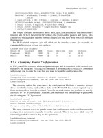
The distributed storage space that each node may allocate is 1492(–27) * 256 ϭ

375 Kbytes. How many IPv4 prefixes do fit in those 375 Kbytes? Figure 12.11 in Chapter
12 “IP Reachability Information” illustrates the structure and storage requirements of the
Extended IP Reachability TLV #135. Worst case, the TLV consumes 9 bytes and best
case 5 bytes due to variable prefix length packing. For the average Internet route we can
assume a prefix length between /16 and /24 and safely assume a total storage requirement
of 8 bytes per prefix. In a single TLV, on average, 31 TLVs fit, which requires 31 * 8 + 2
(TLV Overhead) ϭ 250 bytes to store. An LSP fragment is at maximum 1492 bytes in
size. For TLV information there is 1492 – Header size (ϭ27) ϭ 1465 space. That means
in total we can store 31 * 5 + 26 ϭ 181 routes per fragment. Inside 256 fragments we can
store around 46 K routes, which is too little to hold the entire Internet routing table. As
soon as the routers hit that limit, it pulls the “emergency brake” and sets the overload bit.
472 15. Troubleshooting
Finally, it cleans up the mess by purging the previously generated LSPs off the distrib-
uted link-state database. And that’s what the router was showing us.
In order to fix the problem, the then accept statement is moved into the term
static.
JUNOS configuration
hannes@Munich> show configuration
[… ]
policy-statement static-to-isis {
term reject_management {
from {
route-filter 10.0.0.0/8 orlonger;
}
then reject;
}
term static {
from protocol static;
then accept;
}

}
After committing the change, you will still see all those stale fragments in the data-
base. They will be kept in the database until the garbage collection timer times out. Using
default values, after a period of 20 minutes they are removed automatically.
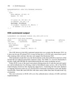
JUNOS command output
After the router has changed, the broken routing policy the Overload Bit is automatically
cleared.
hannes@Munich> show isis database
IS-IS level 2 link-state database:
LSP ID Sequence Checksum Lifetime Attributes
Munich.00-00 0x1c2 0x2d3b 1192 L1 L2
Pennsauken.00-00 0xc77 0xec5e 711 L1 L2
Frankfurt.00-00 0x198 0xdd86 933 L1 L2
14 LSPs
[… ]
The database looks normal again, and the Overload Bit has automatically been
cleared.
Because that problem was encountered many times in the field, Juniper Networks
finally introduced a prefix-export limiter that optionally controls the export behaviour
and suspends route export if a predefined threshold is reached.
Case Studies 473
474 15. Troubleshooting
JUNOS configuration
The prefix-export-limit knob protects the rest of the network from a malicious
policy by applying a threshold filter for exported routed.
hannes@Munich> show configuration
[… ]
protocols {
isis {
export static-to-isis;

level 2 {
wide-metrics-only;
prefix-export-limit 2500;
}
}
}
The amount of prefixes heavily depends on the size of your network. Good design
advice is to set it to double the total number of IS-IS Level 1 and Level-2 routers in your
network – The minimum number of routes should be 1000 and the maximum number of
routes about 10,000. Then you have some growth for even larger numbers of routes that
need to get leaked from Level 1 to Level 2.
15.4 Summary
Most IS-IS problems can be resolved quickly if you stick to a troubleshooting plan and
check from Layer-1 of the OSI Reference Model right up to the Application Layer. In
IS-IS, the Application Layer represents the link-state database that holds the network’s
link state PDUs. The network engineer needs to develop an understanding of what func-
tions each layer is performing and what tools he has available to gather information.
After information gathering, the collected data needs to be analyzed and interpreted,
which requires knowledge of the show commands and debug outputs. For detecting mis-
configuration on a router, the network engineer needs to understand where the IS-IS rele-
vant data in the configuration are stored.
The majority of IS-IS problems are related to adjacency formation. The network engineer
needs to get familiar with all sorts of debug output for IOS and JUNOS. Just looking at
the IS-IS specific configuration is often not enough to resolve a problem. We have
demonstrated in the Internet route export case study that understanding of route export
and policy processing is paramount for resolving complex problems.
16
Network Design
For a long time, link-state protocols were believed not to scale. However, today there are
operational networks with more than 1200 routers in a single level. Still, networks that run

link-state protocols need to be carefully designed and a lot of factors need to be considered
to get to such a scale. By ignoring certain reasonable constraints, you can easily break a
network in certain scenarios. In this chapter you will learn about the critical IS-IS network
design factors, all forms of router stress, including flooding stress, SPF stress and forward-
ing state change stress, as well as what things to consider to build robust, fast-converging
networks.
16.1 Topology and Reachability Information
In service provider networks there are always at least two protocols in use. The first is an
IGP (which could be OSPF or IS-IS), and the other is BGP. One of the first questions
asked by networking novices is why do we need both? It turns out that all IGPs (IS-IS,
OSPF, EIGRP) lack one fundamental thing, which is flow-control. For IGPs, there is no
way to tell an adjacent router that their updates have overwhelmed the receiver and the
sender should throttle down. The only way to deal with the situation is to throw away the
updates and wait for re-transmission. However, that is still a dangerous game, as it may
offload stress at the expense of the sending router, which needs to queue retransmissions
and therefore consumes CPU and memory. Careful protocol heuristics need to be imple-
mented to make sure that both the sending and receiving router do not take themselves
out of service. Dave Katz, a software engineer with Juniper Networks, who can be
blamed for writing the majority of IGP implementations on the Internet (his own self-
definition) puts the complexity around finding the right heuristics in a single quote:
Link State Protocols are hard! (Dave Katz)
What network engineers at service providers have been doing is to apply a divide and
conquer strategy and separating topology from reachability information. Topology infor-
mation contains the skeleton of the network – it is a graph that describes how the routing-
nodes are connected to each other. It does not contain any information about customer
networks and server networks, or so on. Ideally, it does not even contain information
about the directly connected sub-nets. Figure 16.1 shows that the only information that the
routers advertise is their loopback IP address, which is necessary to bring up an iBGP full-
mesh distribution network which handles bulk transport of the routing information.
475

476 16. Network Design
When you run IS-IS over a link you typically advertise your local IP sub-net in your
IS-IS LSPs. There is even the notion that local IP sub-nets should not be announced by
IS-IS, but rather by BGP. Historically there has not been an option to preclude certain IP
sub-nets from being announced. However, recent routing software allows you to change
BGP
BGP
BGP
BGP
BGP
BGP
Washington
IS-IS
IS-IS
IS-IS
IS-IS
IS-IS
IS-IS
192.168.1.11/32 172.16.33.0/24
Pennsauken
192.168.1.18/32 172.16.33.0/24
New York
192.168.1.12/32 172.16.33.0/24
London
192.168.1.17/32 172.16.33.0/24
192.168.1.13/32 172.16.33.0/24
Frankfurt
192.168.1.14/32 172.16.33.0/24
Paris
FIGURE 16.1. The minimal routing information that IS-IS needs to provide is the /32 of the

Loopback IP address for bringing up the iBGP mesh. All customer routes are packed on BGP
that behaviour. In IOS, there is a single knob that changes the advertising behaviour of
directly connects sub-nets. Once you configure the passive-only knob, the routing
software walks down the list of configured interfaces and looks for interfaces that are
marked as passive. Recall that passive means that you include that interface’s
sub-net in your routing update, but you do not try to establish a neighbour relationship or
an adjacency over that interface. The loopback interface is by default passive and so
if you configure the passive-only option, only the loopback IP address of the router
is advertised in its LSP.
IOS configuration
In IOS controlling whether directly connected route get advertised is provided using the
passive-only knob.
New-York# show running-config
[… ]
router isis
advertise passive-only
!
[… ]
In JUNOS there is no specific knob to control advertising behaviour. In JUNOS you
write a policy for achieving that task. Later you call that policy as export policy in the
protocols isis {} branch.
JUNOS configuration
In JUNOS you need to write an explicit policy that rejects all routes beside sub-nets on the
lo0.0 interface.
hannes@Frankfurt# show
[… ]
protocols {
isis {
export lo0-only;
[… ]

}
}
policy-options {
policy-statement lo0-only {
term lo0 {
from interface lo0.0;
then accept;
}
term final {
then reject;
}
[… ]
Topology and Reachability Information 477
The nice thing about the JUNOS policy is that you may explicitly control the level to
suppress direct routes by introduction of a to {} statement. The following example
shows how to restrict to the loopback0 interface related routes inside Level 2 LSPs only.
policy-options {
policy-statement lo0-only {
term lo0 {
from interface lo0.0;
to {
protocol isis;
level 2;
}
then accept;
}
term final {
then reject }
}
}

[… ]
}
BGP has perfected flow-control capabilities because it runs on top of the Transmission
Control Protocol (TCP). Flow control at the TCP level is built into the protocol: as soon
as a receiver cannot keep up processing inbound routing updates, it can easily slow down
transmission of acknowledgements or even drop the inbound update and indirectly indi-
cate that the sender should back off and send information at a lower speed. Originally
BGP was intended to process a certain maximum of routes. Yakov Rekhter, an Internet
architect with Juniper Networks relates:
Kirk Lougheed (Cisco Systems) and myself’s goal was to build a routing protocol able
to convey 1000 routes and not fall into pieces – If you consider the total routes being
today in the Internet we pushed the envelope a bit (Yakov Rekhter)
Based on BGP’s superb scaling capabilities, the idea here is to “borrow” the existing
BGP distribution mesh being used for transport of Internet routes for internal routes
as well.
The conclusion as to why you always need two protocols is therefore: IS-IS scales
too poorly for conveying a bulk amount of routes, however, it can quickly discover a
topology and provide routing connectivity between router loopback IP addresses. BGP
heavily depends on these IGP-supplied routes to bring up the iBGP. Second, BGP is
really in the dark when it comes to ascertaining the distance between a pair of routers.
Internal BGP sessions are not “targeted” and therefore need an IGP to resolve routes and
to give BGP speakers directions.
In order to come up with a design recommendation, let’s first evaluate the forms of
stress that routers are exposed to and develop a set of critical design factors based on
those insights. From there we will set up some rules to follow when designing an IS-IS
network.
478 16. Network Design
16.2 Router Stress
Generally routing software can exhaust resources in three possible areas:
1. Bandwidth

2. CPU
3. Memory
The next three sections investigate IS-IS implementations to see if they suffer from any
limitations in those three areas. The first area is bandwidth – in IS-IS, the main band-
width consumer is related to the flooding of LSPs.
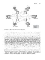
16.2.1 Flooding
Unlike link-local packets like Hellos (IIH) or Synchronization packets (SNP), transmit-
ting link-state PDUs (LSPs) has a network-wide bandwidth usage impact. Once a router
floods LSPs, it is using bandwidth equal to the number of links in a given topology times
the size of the LSP. Worst case, it can be that network-wide transmission of an LSP
comes at a cost of using the number of all links times the size of a LSP squared. The big
gap between the best and the worst case (recall the best case is linear behaviour and the
worst case is N^2 behaviour) is solely explainable by the way the topology is meshed.
Consider Figure 16.2, where in a strict ring topology of six routers there is no duplicate
Router Stress 479
Paris
Ring Topology Full-mesh Topology
Pennsauken
New York
Washington
Frankfurt
London
Pennsauken
New York
Washington
Paris
Frankfurt
London
FIGURE 16.2. In a dense-meshed environment there are lots of duplicate LSPs to process
transmission of an LSP. As soon as a link breaks, the LSP travels round until every node

gets a copy. Note that for greater visibility the propagation of only one LSP is shown. Of
course, in real networks both ends of the link that breaks would originate a new LSP. As
soon as you add links to the topology, the more redundant the transmission of LSPs gets.
In the ring-topology each router sees the LSP one time.
The worst case is a full-mesh of all routers, where a single router failure triggers
(N – 1) LSPs being flooded over (N – 2) links (ϭ O(N
2
)) through the network. The big
problem in a dense- or full-mesh environment is that nodes that already got a copy of
LSPs receive many redundant duplicates with the same information.
An additional source of flooding stress comes from turning on the TE extensions.
Once you turn on features like Traffic Engineering, DiffServ Traffic Engineering or Auto
Bandwidth, then the TEDs throughout the network topology need to be updated through
the use of the IS-IS flooding sub-system. That means that every router in the network
sees (and needs to see) accurate TE information. However, if the TE implementation
permits changes to flooding timers, then let having very conservative timers guide your
design. TE extensions are a major source of LSP updates and there should be an effort to
reduce these to the minimum possible.
It is recommended that you consider the topology to evaluate the stress resulting from
receipt of duplicate LSPs. Densely meshed environments scale poorly in flooding environ-
ments. Try to avoid full-mesh or near-full mesh topologies. Sometimes a lot of extra
redundancy does not turn into more resiliency.
16.2.2 SPF Stress
Link-state routing protocols were once believed to be CPU intense algorithms that
exhausted an embedded system’s sparse resources. Because of that belief, both link-state
IGPs (OSPF, IS-IS) have provisions to split the size of the link-state domains to smaller
units. In OSPF multiple areas, and in IS-IS two levels, are an attempt to spare the control
plane CPU when doing the SPF run.
A lot has changed in the last decade. CPUs became (in line with Moore’s Law) faster by
a factor of 8000; Trunk bandwidth grew from T1 speeds to OC-192c/STM-64. The only

thing that has not changed at all is the paranoid thinking that SPF may exhaust the CPU
resources of a router. The fact is, the demand that SPF puts on router resources has been
outpaced by the processing power of modern CPUs. Table 16.1 shows how SPF execution
fares on modern route processors like the Cisco Systems GRP or a Juniper Networks RE
3.0. The CPU requirements of an SPF operation are well understood and well documented
by computer scientists. The fundamental relationship is O(N
*
log(N )), which describes a
curve where the CPU requirements grow a little more than linearly, with N being the num-
ber of total routers in the network. In practice it is a little more than just log N due to the
2-way check that is needed to verify that a node is connected on both ends and not a dead end.
The results from the simulation in Table 16.1 are impressive. It means that processing
a grid of 2000 routers, which are in total connected by 5000 links, has a typical execu-
tion runtime of only 100–245 milliseconds. If you consider this table then it is obvious
that raw SPF execution time is not a problem for large IS-IS networks. So what is it then?
480 16. Network Design
Why are we all so scared of routers running excessive number of SPF runs back to back?
What is it besides the SPF calculation itself that scares network operators so much?
16.2.3 Forwarding State Change Stress
The purpose of the SPF calculation is to find out the shortest path to every edge of the
network. However, just the insight that there are better paths available is not enough.
There are no good things, unless you do them! (Erich Kästner)
The router has to pass on the new proximity results to a subsystem called the resolver,
which is used to map third party next-hops to forwarding next-hops. Consider Figure
16.3, if the link between Washington and New York breaks, the SPF calculation will be
finished in a matter of microseconds. Each IS-IS speaker is also a BGP speaker and car-
ries several thousand active BGP routes. If the IS-IS topology changes, then the BGP
routes that depend on IS-IS need to get changed as well. The resolver needs now to back-
track through all the BGP routes and verify that the BGP next-hop is affected by a change
in the core topology. As you can imagine, walking down a table of several hundreds of

thousands of BGP route-entries is a resource intensive task. In our example, there are
tons of forwarding state changes to do: all Washington and New York routes need to be
changed in a very short time.
After the BGP dependencies have been worked out, this may generate changes in the
BGP topology as well: recall that the IGP distance is part of the BGP route selection
process. But that is only half of the story, as those things still occur on the control plane.
Router Stress 481
TABLE 16.1. Modern route processors can calculate topologies for
thousands of nodes and links sub second.
SPF runtime (ms)
Juniper Networks Cisco Systems
Routers Links Routing Engine 3.0 GRP 12000
100 250 1,92 4,80
200 500 4,97 12,42
400 1000 12,49 31,22
600 1500 21,18 52,94
800 2000 30,67 76,67
1000 2500 40,78 101,94
1500 3750 68,11 170,27
2000 5000 97,68 244,21
2500 6250 128,98 322,45
3000 7500 161,69 404,22
4000 10000 230,53 576,33
5000 12500 303,09 757,72
6000 15000 378,67 946,67
7000 17500 456,82 1142,04
8000 20000 537,19 1342,98
9000 22500 619,55 1548,86
10000 25000 703,67 1759,18
The forwarding state change of tens of thousands of routes may stress several sub-systems

of an Internet core router. It turns out that changing a forwarding state is one of the most
expensive operations in a router. Meanwhile, both Juniper and Cisco have found a way to
pass on third party next-hop information to the line-cards and retain the dependency of
BGP routes to IS-IS speakers to forwarding interfaces. More on passing on third party next-
hop information, and why it is not always a good idea to attempt to fully resolve a route to
its forwarding next-hop, can be found in Chapter 10, “SPF and Route Calculation”.
482 16. Network Design
Wash D.C.
Metric 4
Metric 2
Metric 4 Metric 2
Metric 1Metric 1
Metric 4 Metric 4
Pennsauken
Frankfurt
London
Washington
New York
Paris
BGP
40 K active
routes
BGP
25 K active
routes
BGP
30 K active
routes
BGP
15 K active

routes
BGP
20 K active
routes
BGP
10 K active
routes
FIGURE 16.3. The resolver needs to track and map BGP next-hops to the shortest path resulting
from the SPF calculation
16.2.4 CPU and Memory Usage
The two main things that utilize the CPU most in an IS-IS router are the SPF calculation
and the resolver. SPF calculation puts a short burden on the system but even in large
topologies that burden does not last more than 200 ms using modern route processors. As
discussed in the previous section, the far bigger CPU hog is the resolver, which maps BGP
routes to forwarding next-hops. SPF execution runtime is ultimately a non-issue; however,
the burden that the resolver can put on the system needs to be carefully examined.
In the 1990s, during the explosive growth of the Internet, routers were constantly short
of memory. Since then network service providers are cautious about the memory usage
of their routing protocols. There is almost no IS-IS-related documentation regarding
memory consumption. The majority of IS-IS implementations use memory in three
areas:
1. Link-state database
2. SPF result table
3. Storing neighbour information
The link-state database size is the easiest to predict. It contains mostly raw data that
was extracted from the TLVs in an IS-IS PDU. There are also overhead and index struc-
tures so the IS-IS software can quickly traverse the database when it is looking for a cer-
tain LSP. As a rough guideline, one can state that the size of the link-state database is
about double the size that individual LSPs consume on the wire. For example, if the net-
work knows about 100 LSPs with an average length of 400 bytes each, then the size to

store this information in the router software is 100
*
400
*
2 ϭ 80 KB.
The size of the SPF result table depends largely on how many IP prefixes are known
to IS-IS inside the network. A good estimation here is that each prefix consumes about
70 bytes. For example, if you have 1600 IS-IS prefixes in your network, then the mem-
ory consumption on the control plane is 112 KB.
The neighbouring table is the most complex one to calculate as all the flooding state
and retransmission list needs to be kept on a per adjacency basis. That structure is also
dependent on the size of the link-state database, because all the flooding states are tied to
both the LSP and the adjacency. There is a lot of clever pointer work involved here, and
the overhead to do efficient flooding is enormous. A good approximate figure is that this
table is about 50 times the average LSP size multiplied by the number of active adjacen-
cies. For example, if the average LSP is about 400 bytes and the number of adjacencies
is eight, then the memory consumption is 400
*
50
*
8 ϭ 160 K.
If you sum the three memory areas up, then the result for a large network is unlikely
to exceed 4–5 MB in total. In IS-IS, the memory consumption is minimal given that
there are mainly route processors with 256 MB–2 GB memory deployed in the field.
Interestingly, there are large overhead structures in the LSP databases to increase LSP
lookup speed and to keep flooding state even for large numbers of adjacencies. This is just
more evidence that memory consumption for IS-IS networks with big core routers is a
non-issue.
Router Stress 483
16.3 Design Recommendations

Through the years of designing large IS-IS networks, and based on the experience of
NOC engineers and software engineers at the big router vendors, the authors have come
up with the following design tips to design truly scalable networks. Those recommenda-
tions are not rigid, that is, you do not need to follow them all to the letter. To be a good
network designer, you have to find a healthy balance between what the products can do
and what you want to achieve.
The rest of this chapter draws on many of the topics and ideas discussed throughout
this book. There is no need to repeat more than the basics of the discussions, however, so
we don’t present all of the gory details all over again.
16.3.1 Separate Topology and IP Reachability Data
Perhaps the most important rule is keeping topology and IP reachability data separate.
You saw that IGPs are not very good at transporting large numbers of routes, so just
avoid it and pass the job to BGP. In large (more than 1000 routers per level) you may
even decide to advertise directly connected routes in BGP as well. Given that an average
IS-IS core router has about five or six directly attached sub-nets, then you clearly want to
avoid that extra 2500–3000 prefixes at the IS-IS level in order to keep convergence times
within an upper bound. An ideal IS-IS LSP contains just a single IP prefix, which is the
router’s loopback IP address, plus Extended IS Reach TLVs that point to neighbouring
routers.
Tcpdump output
An ideal LSP just conveys a single IP prefix per router and passes all other routing infor-
mation via BGP.
12:36:45.587565 OSI, IS-IS, length: 405
hlen: 27, v: 1, pdu-v: 1, sys-id-len: 6 (0), max-area: 3 (0)
L2 LSP, lsp-id: 2092.1113.4009-00, seq: 0x000002fd, lifetime: 1198s
chksum: 0xe984 (correct), PDU length: 185, Flags: [ L1L2 IS ]
Area address(es) TLV #1, length: 4
Area address (length: 3): 49.0001
Protocols supported TLV #129, length: 1
NLPID(s): IPv4

IPv4 Interface address(es) TLV #132, length: 4
IPv4 interface address: 192.168.1.1
Hostname TLV #137, length: 10
Hostname: Washington
Extended IS Reachability TLV #22, length: 99
IS Neighbor: 1921.6800.1077.00, Metric: 4, sub-TLVs present (12)
IPv4 interface address (subTLV #6), length: 4, 172.17.1.6
IPv4 neighbor address (subTLV #8), length: 4, 172.16.1.5
484 16. Network Design
IS Neighbor: 1921.6800.1043.00, Metric: 4, sub-TLVs present (12)
IPv4 interface address (subTLV #6), length: 4, 172.16.33.38
IPv4 neighbor address (subTLV #8), length: 4, 172.16.33.37
IS Neighbor: 1921.6800.1018.00, Metric: 4, sub-TLVs present (12)
IPv4 interface address (subTLV #6), length: 4, 172.16.33.25
IPv4 neighbor address (subTLV #8), length: 4, 172.16.33.26
Extended IPv4 reachability TLV #135, length: 9
IPv4 prefix: 192.168.1.1/32, Distribution: up, Metric: 0
Authentication TLV #10, length: 17
HMAC-MD5 password: 68e18feb2e29257113e4bb6580169310
16.3.2 Keep the Number of Active BGP Routes per Node Low
Vendors have come up with smart representations of BGP routes and how those routes
depend on IS-IS routes. However, there is one fault condition where even smart route
representations inside a router do not gain us much. If an entire BGP speaker disappears,
then when the BGP speaker goes down the BGP control plane needs to re-route all those
prefixes, which of course takes time. If an IS-IS router is carrying a large number of
active routes, then it takes proportionally longer if that BGP router goes down. Figure
16.4 shows that, on the left-hand side, Washington is a “hotspot” BGP speaker that car-
ries the majority of BGP routes. If this speaker goes down, then you need to re-route all
120 K routes, which can cause a network wide outage of up to 3 minutes. The logical step
is to spread those 120 K routes among several routers as shown on the right-hand side of

Figure 16.4.
In well-developed peering meshes, the average number of routes per border router is
not more than 10 K. In our example, because of a lack of routers, we still did not put more
than 30 K routes per node. In practice, if you receive more than 10 K routes per peer, then
you may need to consider a redundant router and spread the incoming prefixes over the
two redundant routers. Re-routing 10 K prefixes if the active router breaks down can be
done in a matter of 5–10 seconds.
16.3.3 Avoid LSP Fragmentation
IS-IS has plenty of space (precisely 375,040 bytes per LSP) in the distributed database.
Despite this vast amount of information that an individual IS-IS speaker can originate,
you typically do not want to use that storage size – ever. You should try to accommodate
all the information that you need in maxLSPsize (1492) – LSP header (27) ϭ 1465
bytes. There may be a number of additional LSP updates if you cross an LSP boundary
and have to break things up into another segment. Consider Figure 16.5 to see what happens
if you are at the edge of Fragment 0 and an additional adjacency comes up. Router
1921.6800.1018 decides that it needs to break up another segment. Router 1921.
6800.1018 generates the fragment and floods it. The troubles start if any of the router’s
other sub-nets or adjacencies become unavailable. Assume that Adjacency #4 falls down,
and then the entire TLVs that follow this particular adjacency gets shifted, and also may
fall into another fragment. Considering the example in Figure 16.5, there is no need to
Design Recommendations 485
486
Frankfurt
London
New York
Frankfurt
London
BGP
BGP
BGP

BGP
BGP
BGP
BGP
BGP
Pennsauken
20K active
routes
120K active
routes
Washington
Paris
20K active
routes
Pennsauken
30K active
routes
New York
30K active
routes
Washington
20K active
routes
Paris
25K active
routes
15K active
routes
F
IGURE

16.4. In a well-developed peering mesh the BGP routes are almost e
venly distributed over the entire network
487
TLVs
Extd-IS Reach Neighbour #1
Extd-IS Reach Neighbour #2
Extd-IS Reach Neighbour #3
Extd-IS Reach Neighbour #4
Extd-IS Reach Neighbour #5
Extd-IS Reach Neighbour #6
Extd-IS Reach Neighbour #7
Extd-IS Reach Neighbour #8
Extd-IS Reach Neighbour #9
Extd-IS Reach Neighbour #10
LSP 1921.6800.1018.00-00,
Sequence 0x1,
Lifetime 1200s
LSP 1921.6800.1018.00-01,
Sequence 0x1,
Lifetime 1195s
TLVs
Extd-IS Reach Neighbour #11
TLVs
TLVs
1
2
Extd-IS Reach Neighbour #1
Extd-IS Reach Neighbour #2
Extd-IS Reach Neighbour #3
Extd-IS Reach Neighbour #4

Extd-IS Reach Neighbour #5
Extd-IS Reach Neighbour #6
Extd-IS Reach Neighbour #7
Extd-IS Reach Neighbour #8
Extd-IS Reach Neighbour #9
Extd-IS Reach Neighbour #10
Extd-IS Reach Neighbour #1
Extd-IS Reach Neighbour #2
Extd-IS Reach Neighbour #3
Extd-IS Reach Neighbour #4
Extd-IS Reach Neighbour #5
Extd-IS Reach Neighbour #6
Extd-IS Reach Neighbour #7
Extd-IS Reach Neighbour #8
Extd-IS Reach Neighbour #9
Extd-IS Reach Neighbour #10
Extd-IS Reach Neighbour #11
LSP 1921.6800.1018.00-00,
Sequence 0x2,
Lifetime 1195s
LSP 1921.6800.1018.00-00,
Sequence 0x2,
Lifetime 1197s
LSP 1921.6800.1018.00-01,
Sequence 0x2,
Lifetime 1197s
empty TLV block
F
IGURE
16.5. IS-IS fragmentation may cause excess LSP updates if adjacencies w

ander across several fragments
use Fragment #1 now, as everything would easily fit into Fragment #0. Fragment #1 is
tossed using a network-wide purge. The trouble here is that a single change in a router’s
adjacency may cause several fragments to get re-aligned. ISO 10589 recommends spar-
ing the top 10 per cent of LSP space for problem scenarios like this. That is, when an
LSP is built, then only the first 1318 bytes (1465 – 10 per cent) are used for data. The top
10 per cent are reserved to take up “wandering adjacencies” from higher fragments as
those fragments shrink below a 146-byte fill level.
There is a lot of clever heuristics involved (you could even pad lost adjacencies using
the Padding TLV #8 in order to avoid fragment shifts); however, most implementations
keep those heuristics to a minimum. In order to avoid fragment shifts, the best approach
is to avoid fragmentation at all.
Tcpdump output
An adjacency carrying full TE extensions consumes 75 bytes on the wire.
Extended IS Reachability TLV #22, length: 75
IS Neighbor: 2092.1113.4007.00, Metric: 5, sub-TLVs present (64)
IPv4 interface address (subTLV #6), length: 4, 172.16.1.6
IPv4 neighbor address (subTLV #8), length: 4, 172.16.1.5
Unreserved bandwidth (subTLV #11), length: 32
priority level 0: 9953.280 Mbps
priority level 1: 9953.280 Mbps
priority level 2: 9953.280 Mbps
priority level 3: 9953.280 Mbps
priority level 4: 9953.280 Mbps
priority level 5: 9953.280 Mbps
priority level 6: 9953.280 Mbps
priority level 7: 9953.280 Mbps
Reservable link bandwidth (subTLV #10), length: 4, 9953.280 Mbps
Maximum link bandwidth (subTLV #9), length: 4, 9953.280 Mbps
Administrative groups (subTLV #3), length: 4, 0x00000000

If you consider that you almost need no space for IP Reachability-related TLVs, there
is approximately space for 18
*
75 bytes of full-blown adjacencies using the full-set of
TE sub-TLVs, which ought to be enough even for larger core routers.
16.3.4 Reduce Background Noise
IS-IS has the nice advantage over OSPF in that IS-IS can control its own LSP refresh
rate. In IS-IS the max-LSP-age is a countdown function, which is user configurable. That
is, each router is required to refresh its LSP (refresh just means bump the sequence num-
ber and leave the contents unchanged) in less than max-LSP-age. The recommended
value for implementers is to set the max-LSP-age refresh timer to a value less than 300
seconds, but this is very low. The default value of the max-LSP-age is set to 1200 sec-
onds, which is also the recommended value mentioned in ISO 10589. If you keep the
488 16. Network Design
default value, or use the 300 value, you end up tolerating a lot of “refresh noise” based
on the relatively small interval of 1200 seconds (20 minutes). For example, in a network
consisting of 400 routers, this means on average every 3 seconds a network-wide flood
of an LSP from some router even when the network is quiet (there are no link flaps, and
no topology changes, and so on).
Both IOS and JUNOS allow you to change that default value of 1200 seconds to get
to a lower amount of refresh noise in your network. The recommended value is to set
the max-LSP-age timer to 65,535 seconds, which extends the refresh period to 18.2
hours and therefore reduces the refresh noise by a factor of 50. There are no side-effects
of changing the default value, and it remains an open question for router vendors as to
why this higher value is not made the default value, because every service provider
changes it to this value anyway. Keep in mind that in IOS you need to set both the lsp-
age timer as well as the lsp-refresh timer and subtract the 300 seconds to get a
proper refreshing. JUNOS internally calculates a “sane” timer based on the configured
lsp-age.
16.3.5 Rely on the Link-layer for Fault Detection

Many service providers believe that the key for getting to sub-second convergence is to
tweak all the timers in a router, particularly the Hello and Hold timers. Unfortunately
today some implementations of routing protocols are not real-time capable. If you make
your non-real-time capable IS-IS implementation generate a Hello every 333 ms on hun-
dreds of adjacencies, this may cause some side-effects. Consider the processing of a big
BGP batch run, where the router may not be able to revisit the code that submits the
Hellos, which in turn may cause network-wide churn due to missed Hellos.
Considering that not all vendors support real-time control planes for IS-IS, we have to
go down the road of the lowest common denominator. In many router implementations,
generation of link-layer messages like keep-alives are handled by the forwarding complex,
which typically does run a real-time OS (or at least a tweaked OS that is close enough). In
order to get real-time detection, we offload this task to the forwarding complex. Fault
detection works reasonably well on certain interface technologies like SONET/SDH. No
surprise here! SONET/SDH have the best liveness protocol you can think of. Among the
SONET/SDH overhead are bytes (K1/K2, K3, K4) that carry Remote Defect Indicator
(RDI) bits which are immediately set if there is a problem along the SONET/SDH link.
Due to SONET/SDH requirements, that message will be sent, worst case, within 50 ms of
a failure and travel through every node along the path.
In the ATM world, end-to-end fault detection is performed by operation and manage-
ment (OAM) cells that are inserted by routers at both ends of a Virtual Connection (VC).
The OAM cells are a nice liveness protocol that can perform fault-detection for IS-IS
as well.
The only remaining problem is Ethernet. Because of its inherent simplicity, there is no
link-layer protocol where you could embed Ethernet keep-alive messages. Historically there
was never any possibility to get quick fault detection on Ethernet except through tuning
IS-IS Hold timers. But now there is a solution called bi-directional fault detection (BFD) for
this purpose. BFD is described in draft-katz-ward-bfd-00.txt and the protocol and its
Design Recommendations 489
mechanisms are simple: The idea is to set up a high frequency (Ͻ100 ms) exchange of UDP
packets. If that exchange is disrupted there must be a problem with the underlying media and

the link can be declared down. As soon as there are interoperable BFD implementations it
will become the method of choice as a liveness protocol for Ethernet.
Table 16.2 shows a short summary of the preferred interface media type fault-
detection protocols over IS-IS.
As for every major interface type there is a high-frequency fault detection protocol
available and so there is no need to abuse IS-IS to provide that function. It is our recom-
mendation to use the per-interface media type-dependent fault-detection protocols and
leave IS-IS with its default Hello timers.
16.3.6 Simple Loopback IP Address to System-ID
Conversion Schemes
The 6-byte System-ID field has an inherent drawback. For administering System-IDs
there are almost no address management tools available that can cope with 6-byte
address entities. For the network service operator there are two choices:
1. Develop a custom address management tool for 6-byte System-IDs
2. Do not manage System-IDs – rather auto-derive it from IPv4 loopback addresses
Typically, network service providers do not want to maintain yet another list of addresses,
and therefore there are very simple mapping concepts for converting IPv4 loopback
addresses to System-IDs. It is recommended to keep these schemes as simple as possible.
The simplest form is the binary coded decimal (BCD) conversion where the IP address
is represented in decimal notation and the resulting digits make up the System-ID. See
Figure 16.6 for a few conversion examples.
490 16. Network Design
TABLE 16.2. For every interface media type there is a
high-frequency fault-detection protocol available.
Interface media type Liveness protocol
SONET/SDH SONET/SDH RDI
ATM OAM cells
Ethernet Bi-directional fault detection
192.168.13.1
193.83.223.237

172.1.14.18
IP Address
System-ID
1921.6801.3001
1930.8322.3237
1720.0101.4018
FIGURE 16.6. The best conversion tool is a simple binary coded decimal (BCD) conversion
Simple System-ID schemes also have the advantage that once you need to troubleshoot
complex synchronization and flooding problems, it is convenient to have simple schemes
to spot on certain routers.
Tcpdump output
When you are (for example) troubleshooting a synchronization problem, then it is handy if
you can easily derive the IPv4 address of routers by use of a simple mapping scheme.
21:14:07.712478 OSI, IS-IS, length: 1478
L2 CSNP, hlen: 33, v: 1, pdu-v: 1, sys-id-len: 6 (0), max-area: 3 (0)
source-id: 6b01.c219.07fa.00, PDU length: 275
start lsp-id: 1921.6800.1001.00-00
end lsp-id: 1921.6800.1039.00-00
LSP entries TLV #9, length: 240
lsp-id: 1921.6800.1001.00-00, seq: 0x00000562, lifetime: 5014s,
chksum: 0x03dc
lsp-id: 1921.6800.1003.00-00, seq: 0x0000073a, lifetime: 31107s,
chksum: 0xdb8b
lsp-id: 1921.6800.1005.00-00, seq: 0x0000050c, lifetime: 5205s,
chksum: 0xa8bf
lsp-id: 1921.6800.1006.00-00, seq: 0x00000d20, lifetime: 30639s,
chksum: 0x2699
lsp-id: 1921.6800.1007.00-00, seq: 0x0000089f, lifetime: 52194s,
chksum: 0x74ad
lsp-id: 1921.6800.1011.00-00, seq: 0x00000319, lifetime: 61707s,

chksum: 0xc69e
lsp-id: 1921.6800.1011.00-01, seq: 0x0000008e, lifetime: 44126s,
chksum: 0x6e4d
lsp-id: 1921.6800.1013.00-00, seq: 0x000002c0, lifetime: 36610s,
chksum: 0xb05d
lsp-id: 1921.6800.1013.00-01, seq: 0x000000b0, lifetime: 5052s,
chksum: 0x0e21
lsp-id: 1921.6800.1013.00-03, seq: 0x0000029f, lifetime: 11790s,
chksum: 0x5bfa
lsp-id: 1921.6800.1033.00-00, seq: 0x00000318, lifetime: 11255s,
chksum: 0xbb6e
lsp-id: 1921.6800.1034.00-00, seq: 0x000006f4, lifetime: 48962s,
chksum: 0x634f
lsp-id: 1921.6800.1037.00-00, seq: 0x000005bf, lifetime: 44818s,
chksum: 0x4701
lsp-id: 1921.6800.1038.00-00, seq: 0x000013fc, lifetime: 8664s,
chksum: 0x93d4
lsp-id: 1921.6800.1039.00-00, seq: 0x000014b9, lifetime: 17862s,
chksum: 0x2894
Particularly when you need to parse packet dumps like the above using network ana-
lyzers, and you do not have the name cache ready, then simple conversion logic makes
Design Recommendations 491
troubleshooting much easier. You are doing operations and support people a big favour if
you avoid fancy and complicated System-ID schemes.
16.3.7 Align Throttling Timers Based on Global Network Delay
In most IS-IS implementations there are many timers that the network operator can
adjust. In order to build a network that converges in the sub-second range, you often need
to tweak those timers. The first thought may be the faster the better, however, that’s not
always the case. The typical throttles that are on by default are LSP origination and SPF
delay timers. Both JUNOS and IOS have a similar strategy to apply these throttles. Both

implementations in common behave fast (almost no delay) for the first events in a series.
However, the more quickly changes come, the more restrictive, and hence slower, the sys-
tem behaves. This is achieved as a step function in JUNOS (the first three events are han-
dled the fast way, and then the system immediately backs off to slow behaviour) and in
IOS the router gets slower using an exponential curve. However, after three or four events,
the system fully backs off to the slower behaviour. The art of good network design is to
find a healthy compromise so that the majority (95 per cent) of network events falls under
the fast window and you can take full advantage of the open throttles. Consider Figure
16.7. When parts of a network fail, then there is always more than one LSP in flight. Once
the link between Washington and New York breaks, both routers have to update their
LSPs. Ideally both LSPs arrive at all the routers at the same point in time.
Now you need to find a compromise between reasonably fast behaviour and waiting
long enough that you can catch and process an SPF run for all the LSPs belonging to a
particular network fault condition. How long is long enough? If you take a closer look at
how an incident is processed, then the dominating element after mutual detection of a
link-break is the propagation of the LSP. LSP propagation with reasonably fast circuits
(greater then OC-3/STM-1 speeds) is mostly a function of the light-speed in a fibre plus
the LSP processing delay of routers. A good estimation for the average global flooding
delay is the worst case delay for network control traffic, plus the average hop count, multi-
plied by 10 ms (average LSP processing delay).
Speed of light in fibres is about 200.000 km/s ϭ 200 km/ms
Example 1: Continental network (diameter 4.000 km) spanning over average 6 routers.
4.000 km/200 km/ms ϩ 6 * 10 ms ϭ 20 ms ϩ 6 * 10 ms ϭ 80 ms
Example 2: Intercontinental network (diameter 30.000 km) spanning over an average of
8 routers.
30.000 km/200 km/ms ϩ 8 * 10 ms ϭ 150 ms ϩ 8 * 10 ms ϭ 230 ms
It is recommended to change the LSP origination timer to a value that safely catches most
link flaps. It should not be set too aggressively. A good recommendation here is 150 ms,
which gives the router enough time to fully build an LSP no matter how large it may be.
It is recommended that you change the SPF delay timer based on the calculation for

the average processing and LSP propagation delay. A recommendation for delaying the
SPF calculation is between 50 ms and 250 ms depending on network size.
492 16. Network Design
Design Recommendations 493
New York LSP
Washington LSP
Pennsauken
Frankfurt
London
Washington
New York
Paris
FIGURE 16.7. For true fast-convergence routing the throttling behaviour should match the LSP
propagation properties of the network
16.3.8 Single Level Where You Can – Multi-level
Where You Must
IS-IS has many useful scaling tools built in. One of them is the multi-level orientation
that allows having hundreds of routing domains composed of hundreds of routers and
routes between them. An important question to ask yourself is how much scalability
do you really need? A couple of years ago, everybody in the communication industry was
494 16. Network Design
crazy over scaling, and even pushing the envelope for scalability was not enough for
some network service providers. Fortunately today some normality (some say sanity) has
come back to the industry, and most people now realize their true scaling needs and the
associated time-span until a next generation of network and network routers are needed.
According to our experience, for the majority of networks, there is a simple design rule,
which is to start with a single level of IS-IS. Unless your topological domain (IS-IS level)
grows to a total number of beyond 800–1500 routers, there is no need to split things up.
Do not be misled and think that splitting up a single level network into a multi-level net-
work must automatically improve the scaling properties in all dimensions of that net-

work. There are some examples where the additional complexity of processing two
topological domains may result in worse resource demands. A good case study is shown
in Figure 16.8. In a given multi-level network, in order to still get optimal BGP routing,
you need to turn on route leaking and propagate all /32 loopback routes. An individual /32
prefix originating in Area 49.0100 Level 1 is leaked up to the Level 2 Area 49.0001 and,
due to route leaking, it will be propagated down to Area 49.0200 Level 1. If you now sup-
pose (for example) that the San Francisco router goes down, then the timing properties
of all the individual operations are:
1. Flood inside Level 1 Area 49.0100 (20ms)
2. Atlanta: SPF delay, local SPF calculation, leak to Level 2, LSP build delay
(100 ms ϩ 10 ms ϩ 100 ms)
3. Flood inside Level 2 Area 49.0001 (20 ms)
4. Amsterdam: SPF delay, local SPF calculation, leak to Level 1, LSP build delay
(100 ms ϩ 10 ms ϩ 100 ms)
5. Flood inside Level 1 Area 49.0200 (20 ms)
6. Stockholm: SPF delay, local SPF calculation (10 ms ϩ 10 ms)
If you sum up all of these operations then the total Level-1-to-Level-1 convergence
takes 500 ms compared to the single level flooding delay, plus SPF delay and SPF calcu-
lation (130 ms). Although the network should behave better, it actually got worse by a
factor of 4 in terms of convergence.
Typically, you start a green-field design with a single Level-2 IS-IS network. You may
ask why to start with Level 2 first and not with Level 1, and extend it later to a Level-2
network? Figure 16.9 shows the two transitioning examples. On the top, the migration
from a Level-2 to a multi-level network works without any disruption at all. Only two
level settings need to be changed. On the bottom the conversion from a Level-1 to Level-
2 is troublesome, because Level-1 adjacencies require that the Area address matches on
both ends, and in order to create several Level-1 areas you need to renumber the areas
and touch every router. This means that for a short time you must disrupt your service. In
the top example we assume that the network administrator has allocated the appropriate
distinct Area-IDs so that they can change the level anytime. In Level 2 routing, different

Area-IDs are tolerated – the Area-ID does not need to match. A little piece of tolerance
is generally a good recipe for easy transitioning, and here it helps to be able to renumber
the Area-IDs without any disruption. That is good news, as you do not need to worry
about addressing from the start. You can at a later stage change the entire IS-IS Area
addressing and add anything at any time.
495
Frankfurt
London
Washington
New York
Paris
Miami
San Jose
Vienna
Munich
Amsterdam
Atlanta
San Fran
Area
49.0100
Area 49.0001
Level 2-only
Pennsauken
Stockholm
Area 49.0200
F
IGURE
16.8. In a two level IS-IS network propagation through all levels does slo
w down convergence
2

2
2
2
1
1
1
1
1
2
2
1
1
2
2
1
Amsterdam
London
Atlanta
New York
Amsterdam
London
Atlanta
New York
Amsterdam
London
Atlanta
New York
Amsterdam
London
Atlanta

New York
49.0100
Pennsauken
49.0001
Level 2-only
49.0200
Multi Level
49.0100
Pennsauken
49.0001
49.0200
Level 1-only
49.0001
Pennsauken
49.0100
Pennsauken
49.0001
49.0200
Multi Level
F
IGURE
16.9. Level 2-only to multi-level
transition is easier than
Level 1-only to multilevel
, as it does not require renumbering Area-IDs
496