Mạng VSAT (P2) ppsx
Bạn đang xem bản rút gọn của tài liệu. Xem và tải ngay bản đầy đủ của tài liệu tại đây (1.34 MB, 32 trang )
2
USE
OF
SATELLITES
FOR VSAT NETWORKS
It is not
so
important for someone who
is
interested in VSAT networks to know
a lot about satellites. However, a number of factors relative to satellite orbiting
and satellite-earth geometry influence the operation and performance of VSAT
networks. For instance, the relative position of the satellite with respect to the
VSAT at a given instant determines the orientation of the VSAT antenna and also
the carrier propagation delay value. The relative velocity of the satellite with
respect to the earth station receiving equipment induces Doppler shifts on the
carrier frequency that must be tracked and compensated for.
This
impacts on the
specifications and the design of earth station receivers. For a geostationary
satellite, which is supposed to be in a fixed position relative to the Earth, one may
believe that once the antenna has been properly pointed towards that position at
the time of its installation, the adequate orientation is established once and for all.
Actually, as a result of satellite orbital perturbations, there is no such
thing
as
a geostationary satellite, and residual motions induce antenna depointing and
hence antenna gain losses which affect the link performance.
Therefore it is worth mentioning these aspects, and
this
is
the aim of
this
chapter.
Orbit definition and parameters will be presented in the general case, with the
ulterior motive to give the reader some conceptual tools that would be handy
should VSAT networks
be
used some day in conjunction with non-geostationary
satellite systems. However, as current VSAT networks use geostationary satel-
lites, the bulk of the chapter will consider
this
specific scenario. Many of the
considerations developed in this chapter will be used in the following ones.
Before orbital aspects are dealt with,
the
role
of
the satellite and some related
topics will first be introduced as an encouragement to the reader.
2.1
INTRODUCTION
2.1.1
The
relay
function
Satellites relay the carriers transmitted by earth stations on the ground to other
earth stations, as illustrated in Figure
2.1.
Therefore, satellites act similarly to
VSAT Networks
G.Maral
Copyright © 1995 John Wiley & Sons Ltd
ISBNs: 0-471-95302-4 (Hardback); 0-470-84188-5 (Electronic)
50
Use
of
satellites
for
VSAT
networks
SPACE
SEGMENT
UPLINK DOWNLINK
STATION
TRANSMITTING
RECEIVING
EARTH STATION
EARTH STATION
GROUND SEGMENT
Figure
2.1
Architecture
of
a satellite system
microwave terrestrial relays installed
on
the top of hills or mountains to facilitate
long distance radio frequency links. Here the satellite, being at a much higher
altitude than
any
terrestrial relay, is able to link distant earth stations, even from
continent to continent.
Figure
2.1
indicates that the earth stations are part
of
what is called the
ground
segment,
while the satellite is part of the
space
segment.
The space segment also
comprises all the means to operate the satellite, as for instance the stations which
monitor the satellite status by means of telemetry links, and control it by means of
command links. Such links are sometimes called TTC (Telemetry, Tracking and
Command) links.
The satellite roughly consists
of
a platform and a payload. The platform consists
of all subsystems that allow the payload to function properly, namely:
-the mechanical structure which supports all equipments in the satellite;
-the electric power supply, consisting of the solar panels and the batteries used
as supply during eclipses of the sun by the Earth and the Moon;
-the attitude and orbit control, with sensors and actuators;
Introduction
51
-the propulsion subsystem;
-the onboard
TTC
equipment.
The payload comprises the satellite antennas and the electronic equipment for
amplifying the uplink carriers. These carriers are also frequency converted to the
frequency of the downlink. Frequency conversion avoids unacceptable inter-
ference between uplinks and downlinks.
Figure
2.2
shows the general architecture of the payload. The receiver
(W)
encompasses a wide band amplifier and a frequency downconverter. The input
multiplexer (IMUX) splits the incoming carriers into groups within several
sub-bands, each group being amplified to the power level required for trans-
mission by a high power amplifier, generally a travelling wave tube
(TWT).
The
different groups of carriers are then combined in the output multiplexer (OMUX)
and forwarded to the transmitting antenna. The channels associated with the
sub-bands of the payload from IMUX to OMUX are called
transponders.
The
advantage of splitting the satellite band is three-fold:
-each transponder
TWT
amplifies a reduced set of carriers, hence each carrier
benefits from a larger share of the limited amount of power available at the
output of the
TWT;
-the transponder
TWT
operates in a non-linear mode when driven near satura-
tion. Saturation
is
desirable because the
TWT
then delivers more power to the
amplified carriers than when operated in a backed-off mode, away from
saturation. However, amplifying multiple carriers in a non-linear mode gener-
ates intermodulation, which acts as transmitted noise on the downlink. Less
intermodulation noise power is transmitted with a reduced set of amplified
carriers within each
TWT;
spectrum
of
canier
uplink
transponder
bandwidth
\
satellite bandwidth frequency
Figure
2.2
Payload
architecture
52
Use of satellites for
VSAT
networks
-reliability is increased, as the failure of one TWT does not imply an overall
satellite failure and each TWT
can
be backed up.
Typical values
of
bandwidth for a transponder are 36 MHz,
45
MHz, and 72
MHz. However, there is no established standard. The
TWT
power is typically
a few tens of watts. Some satellites are now equipped with solid state power
amplifiers
(SSPA)
instead of
TWTs.
Figure 2.2 does not indicate any back-up equipment. To actually ensure the
required reliability at the end of life of the satellite, some redundancy is built into
the payload: for instance, the receiver is usually backed up with a redundant unit,
which can be switched on in case
of
failure of the allocated receiver. The
transponders are also backed up by a number of redundant units: a popular
scheme is the ring redundancy, where each IMUX output can be connected to any
of several transponders, with a similar arrangement between the transponder
outputs and the OMUX inputs.
2.1.2
Transparent and regenerative payload
A
satellite payload is transparent when the carrier is amplified and frequency
downconverted without being demodulated. The frequency conversion is then
performed by means of a mixer and a local oscillator as indicated in Figure 2.3: the
carrier at a frequency equal to the uplink frequencyf, minus the local oscillator
frequencyf,, is usually selected by filtering at the output of the mixer, and the
local oscillator frequency is tuned
so
that the resulting frequency corresponds to
the desired downlink frequency
f,.
For instance, an uplink carrier at frequency
fu
=
14.25
GHz mixed with a local oscillator frequency
fLo
=
1.55
GHz results in
a downlink carrier frequencyf,
=
12.7 GHz.
A
transparent payload makes no distinction between uplink carrier and uplink
noise, and both signals are forwarded on the downlink. Therefore, at the earth
station receiver, one gets the downlink noise together with the uplink retransmit-
ted noise.
A
regenerative payload entails on-board demodulation
of
the uplink carriers.
On-board regeneration is most conveniently performed on digital carriers. The bit
stream obtained from demodulation of a given uplink carrier is then used to
modulate a new carrier at downlink frequency.
This
carrier
is
noise-free, hence
from
to
IMUX
fD
=
f"
-
f,o
Figure
2.3
Receiver
for
a
transparent satellite
lntroduction
53
I
l4
timc
FDMA
uplink
f
frequency
I4
TDM
downlink
time
Figure
2.4
Regenerative
satellite
payload
with
multiplexed transmission
on
the
downlink
a regenerative payload does not retransmit the uplink noise on the downlink. The
overall link quality is therefore improved. Moreover, intermodulation noise can
be avoided as the satellite channel amplifier is no longer requested to operate in
a multicarrier mode. Indeed, several bit streams at the output of various demodu-
lators can be combined into a time division multiplex (TDM) which modulates
a single high rate downlink carrier.
This
carrier is amplified by the channel amplifier
which can be operated at saturation without generating intermodulation noise as
the carrier it amplifies is unique.
This
concept is illustrated in Figure
2.4.
It should be emphasised that today’s commercial satellites are not equipped
with regenerative payloads but only with transparent ones. Only a few experi-
mental satellites such as NASA’s Advanced Communications Technology Satel-
lite (ACTS) and the Italian ITALSAT incorporate a regenerative payload. The
chances that regenerative payloads will be used in the future to support VSAT
networking
for
commercial services is discussed
in
Chapter
6,
section
6.3.
2.1.3
Coverage
The coverage of a satellite payload is determined by the radiation pattern of its
antennas. The receiving antenna and the transmitting antenna may have different
patterns and hence there may be a different coverage for the uplink and the
54
Use
of
satellites
for
VSAT
networks
GEOSTATIONARY SATELLITE
Figure
2.5
Global
coverage
downlink. The coverage is usually defined by a specified minimum value of the
antenna gain: for instance, the
3
dB coverage corresponds to the area defined by
a contour of constant gain value
3
dB lower than the maximum gain value at
antenna boresight.
This
contour defines the
edge
of
coverage.
There are four types of coverage:
-Global
coverage:
the pattern of the antenna illuminates the largest possible
portion of the surface of the Earth as viewed from the satellite (Figure
2.5).
A
geostationary satellite sees the earth with an angle equal to
17.4'.
Selecting the
beamwidth of the antenna as
17.4"
imposes that the maximum gain at boresight
is
20
dBi, and then the gain at edge of the minus
3
dB coverage is
17
dBi.
-Zone coverage:
an area smaller than the global coverage area is illuminated
(Figure
2.6).
The coverage area may have a simple shape (circle or ellipse) or
a more complex shape (contoured beam). For a typical zone coverage the
antenna beamwidth is of the order of
5".
This
imposes a maximum gain at
boresight of
30
dBi, and a gain at edge of the minus
3
dB coverage of
27
dBi.
lntroduction
55
GEOSTATIONARY SATELLITE
Figure
2.6
Zone
coverage
-Spot
beam
coverage:
an area much smaller than the global coverage area is
illuminated. The antenna beamwidth is
of
the order of
2"
(Figure
2.7).
Con-
sidering a
1.7"
beamwidth imposes a maximum gain at boresight
of
40
dBi and
a gain at edge of the minus
3
dB
coverage
of
37
dBi.
-Multibeam
coverage:
a spot beam coverage has the advantage
of
higher an-
tenna gain than any other type
of
coverage previously discussed, but it can
service only the limited zone within its coverage area.
A
service zone larger
than the coverage area
of
a spot beam can still be serviced with high antenna
gain thanks to a multibeam coverage made
of
several individual spot beams.
An
example
of
such a coverage with adjacent spot beams is shown in Figure
2.8.
This requires a multibeam satellite payload with more complex antenna farms.
Maintaining interconnectivity between all stations
of
the service zone also
56
Use
of
satellites
for
VSAT
networks
2"
GEOSTATIONARY SATELLITE
Figure
2.7
Spot
beam
coverage
implies a more complex payload architecture than that considered in Figure
2.2.
Interconnectivity between stations implies that beams be interconnected: this
can be achieved either by permanent connections from the uplink beams to the
downlink ones, as illustrated in Figure
2.9,
or by temporary connections
established through an on-board switching matrix, as shown in Figure
2.10.
Permanent connections entail a larger number of transponders than on-board
switching. On-board satellite switching requires that earth stations transmit
bursts
of
carriers, synchronous to the satellite switch state sequence, in such a way
that they arrive at the satellite exactly when the proper uplink beam to downlink
beam connection
is
established. More details on the operation
of
such multibeam
satellite systems can be found in [MAR93, Chapter
51.
Introduction
57
n
h
58
Use
of
satellites
for
VSAT
networks
UPLINK DOWNLINK
Ire
uenc
time
frequencq
t
i
rrle
time
frequency
a
:.:.:.:.:.:.:.
.:
.
:.:::::?,
.
BpF
^*I^^-^-
^^^^
^ ^^
t
i
me
I
I
Figure
2.9
Interconnectivity
of
beams
by
permanent connections. (Reproduced
from
[MAR931
by permission
of
John
Wiley
&
Sons
Ltd)
Usually the extension of a
VSAT
network is small enough for all
VSATs
and the
hub station to be located within one beam.
2.1.4
Impact of coverage on satellite relay performance
The relay function of the satellite as described in section
2.1.1
entails adequate
reception of uplink carriers and transmission
of
downlink carriers.
As
will be
demonstrated in Chapter
5,
the ability of the satellite payload to receive uplink
carriers is measured by the figure of merit
Gfl
of the satellite receiver, and its
ability to transmit is measured by its Effective Isotropic Radiated Power (EIRP).
Those characteristics are defined
in
more detail in Chapter
5.
Basically,
Gfl
is the
ratio
of
the receiving satellite antenna gain to the uplink system noise tempera-
ture, and the EIRP is the product of the transmitting satellite antenna gain
G,
and
the power
P,
fed to the antenna by the transponder amplifier. Therefore, both
parameters are proportional to the satellite antenna gain.
The specified values of
GP
and EIRP are to be considered at edge of coverage.
Usually the edge of coverage is definedby the contour on the Earth corresponding
to a constant satellite antenna gain, say
3
dB below the gain
G,,,
at boresight.
Zntroduction
a
60
Use
of
satellites
for
VSAT
networks
Now the maximum satellite antenna gain, Gm,, as obtained at boresight, is
inversely proportional to the square of its half-power beamwidth
03dB:
or
29
000
Gmax
=
-
%B
GmaX(dBi)
=
44.6
-
20
log
e,,
Hence, one can consider that the specified values of
Gfl’
and EIRP are conditioned
by the value of the satellite antenna gain at edge of coverage
G,,
given by:
G
=-
Gmax
em
2
or
G,,(dBi)
=
Gma,(dBi)
-
3
dB
From
(2.2)
and
(2.1),
it canbe seen that the specifiedvalues of Gfl’and EIRP at edge
of coverage are conditioned by the satellite antenna beamwidth
&dB:
the larger the
beamwidth, the lower the G/T and EIRP.
So,
the coverage of the satellite influences its relaying performance in terms
of
Gfl’
and
EIRP.
A
global coverage leads to smaller values
of
satellite
Gfl’
and EIRP,
compared to a spot beam coverage. Should the
VSAT
network be included
in
a single satellite beam, then the larger its geographical dispersion, the poorer the
satellite performance: this has to be compensated for by installing larger
VSATs.
For networks comprised of highly dispersed
VSATs,
say spread over several
continents, the advantages of simple networking in terms of easy interconnectiv-
ity by placing all
VSATs
within a single beam have to be weighed against the cost
of increasing the size of the
VSATs,
which might not be necessary by accepting to
service the network with a multibeam satellite, at the expense, however, of a more
complex network operation.
2.1.5
Frequency reuse
Frequency reuse consists of using the same frequency band several times in such
a way as to increase the total capacity of the network without increasing the
allocated bandwidth.
Frequency reuse can be achieved within a given beam by using polarisation
diversity: two carriers at same frequency but with orthogonal polarisations can be
discriminated by the receiving antenna according to their respective polarisation.
With multibeam satellites the isolation resulting from antenna directivity can be
exploited to reuse the same frequency band
in
different beams.
Figure
2.11
compares the principle of frequency reuse (a) by orthogonal
polarisation, and (b) by angular beam separation. In both cases the bandwidth
allocated to the system
is
B.
The system uses this bandwidth
B
centred on
frequencyf, for the uplink and on the frequencyf, for the downlink. In the case of
Orbit
61
(a)
(W
Figure
2.11
Frequency reuse;
(a)
by orthogonal polarisation; (b) by angular separation
of
the beams
in
a
multibeam satellite system
frequency reuse by orthogonal polarisation, the bandwidth
B
can only be reused
twice. In the case
of
reuse by angular separation, the bandwidth
B
can be reused
for as many beams as the permissible beam to beam interference level allows.
Both types of frequency reuse can be combined.
2.2
ORBIT
2.2.1
Newton’s universal law
of
attraction
Satellites orbit the earth in accordance with Newton’s universal law
of
gravi-
tation: two bodies
of
mass
m
and
M
attract each other with a force which is
proportional to their masses and inversely proportional to the square of the
distance,
Y,
between them:
F=GMY
(N)
m
r
where
G
(gravitational constant)
=
6.672
X
10-”
m3/kg
s2.
orbiting body has a value
As
the mass
of
the Earth is
M,
=
5.974
X
lP4
kg, the product
GM,
for
an earth
p
=
GM,
=
3.986
X
10*4m3/~
2
From Newton’s law, the following results can be derived, which actually were
formulated prior to Newton’s works by Kepler from his observation
of
the
movement
of
the planets around the sun:
-the trajectory of the satellite
in
space, called its orbit, lies in a plane containing
the centre
of
the Earth: for communication satellites, the orbit
is
selected to be
62
Use
of
satellites
for
VSAT
networks
an ellipse and one focus is the centre
of
the Earth. Should the orbit be circular,
then the orbit centre coincides with the Earth's centre;
-the vector from the centre of the Earth to the satellite sweeps equal areas in
equal times;
-the period
T
of revolution of the satellite around the Earth is given by:
T=
271
-
(seconds)
4
where
U
is the semi-major axis of the ellipse
(in
meters).
2.2.2
Orbital parameters
Six parameters are required to determine the position
of
the satellite in space
(Figure 2.12: [MAR93, Figure 7.4, p. 2311):
-two
parameters for the determination of the plane of the orbit: the inclination of
the plane
(i)
and the orbit right ascension of the ascending node
(Cl);
-one parameter for positioning the orbit
in
its plane: the argument of the perigee
(0);
Figure
2.12
Positioning
of
satellite in space. (Reproduced from [MAR931
by
permission
of
John
Wiley
&
Sons
Ltd)
Orbit
63
Figure
2.13
Orbit
plane positioning:
Q,
i
-two parameters for the shape of the orbit: the semi-major axis
(a)
of the ellipse,
and its eccentricity
(e);
-one parameter for the positioning of the satellite on the elliptic curve: the true
anomaly
(v).
2.2.2.1
Plane
of
the orbit (Figure
2.13)
The plane of the orbit is obtained by rotating the Earth's equatorial plane about the
line
of
nodes
of the orbit. The nodes are the intersections of the orbit with the
equatorial plane of the Earth. There
is
one ascending node where the satellite
crosses the equatorial plane from south to north, and one descending node where
the satellite crosses the equatorial plane from north to south. The rotation angle
about the line of nodes is
i,
defined as the
inclination
ofthe
orbital plane.
This
angle is
counted positively in the forward direction between
0"
and
180"
between the
normal
n,
(directed towards the east) to the line of nodes in the equatorial plane,
and the normal
n2
(in the direction of the satellite velocity) to the line of nodes
in
the orbital plane.
The line of nodes must be referenced to some fixed direction in the equatorial
plane. The commonly used reference direction
is
the line of intersection of the
Earth's equatorial plane with the plane of the ecliptic, which is the orbital plane of
the Earth around the sun (Figure 2.14).
This
line maintains a fixed direction in
space with time, called the
direction
of
the vernal point
y.
Actually, as a result of
some irregularities
in
the rotation of Earth, with its axis experiencing nutation, the
direction of the vernal point is not perfectly fixed with time. Therefore the
reference direction is taken as the direction of the vernal point at some instant,
usually noon on January 1, year 2000, designated as
yzm.
The angle which defines
the direction of the line of nodes is the
right ascension
of
the ascending node
R:
it is
counted positively from
0"
to
360"
in the forward direction in the equatorial plane
about the Earth's axis.
64
Use
of
satellites
for
VSAT
networks
equinox
equatorial plane
at
equinox
- -
-
- - - -
hbqn
equinox'
23.5O
\
summer
/
Figure
2.14
The direction
of
the vernal point
y
is used as the reference direction in space
plane
Figure
2.15
Positioning the orbit in its plane: the argument of the perigee
(W)
2.2.2.2 Positioning the orbit in its plane (Figure 2.15)
The centre of the Earth is one of the focuses of the elliptical orbit. Therefore, the
major axis of the ellipse passes through the centre of the Earth. The direction
of
the
perigee in the plane of the orbit
is
determined by the
argument
of
the perigee
W,
which
is the angle, with vertex at the centre of the Earth, taken positively from
0"
to 360"
in the direction of the motion of the satellite between the direction of the ascending
node and the direction of the perigee. The
perigee
is the point of the orbit that is
nearest to the centre
of
the Earth. At the opposite point of the major axis is the
apogee,
which is the point of the orbit that is farthest from the centre of the Earth.
2.2.2.3 Shape
of
the orbit (Figure 2.1
6)
The shape of the orbit
is
determined by its
eccentricity,
e,
and the length,
a,
of its
semi-major axis.
The eccentricity is given by:
C
e
=-
a
The geostationay satellite
65
Perigee
Figure
2.16
Defining the shape
of
the orbit:
U,
e
=
c/u
Perigee
Figure
2.17
Positioning the satellite
in
its orbit
where
c
is the distance from the centre of the ellipse to the centre of the Earth. For
a circular orbit the eccentricity
is
zero, and the centre of the Earth is the centre of
the circular orbit.
The distance from the centre of the Earth to the apogee is
u(1
+e),
and the
distance
from
the centre of the Earth to the perigee is
u(1-
e).
2.2.2.4
Positioning the satellite in its orbit (Figure
2.1
7)
The position of the satellite
in
its orbit
is
conveniently defined by the
true unorndy,
v,
which is the angle with vertex at the centre
of
the Earth counted positively
in
the
direction of movement of the satellite from
0"
to
360°,
between the direction of the
perigee and the direction of the satellite.
The distance from the centre of the Earth to the satellite is given by:
1-2
1
+ecosv
r=u
(m)
The satellite velocity is given by:
2.3
THE GEOSTATIONARY SATELLITE
2.3.1
Orbit parameters
A
geostationary satellite proceeds
in
a circular orbit
(e
=
0)
in the equatorial plane
(i
=
0").
The angular velocity
of
the satellite
is
the same as that of the Earth, and
in
66
Use
of
satellites
for
VSAT
networks
Table
2.1
Characteristics
of
a
geostationary
satellite
orbit
Eccentricity
(e)
0
Inclination
of
orbit
plane
(i)
0"
Period
(T)
23h56min4s=86154s
Semi-major
axis
(a)
42
164
km
Satellite
altitude
(R,,)
35 786
km
Satellite
velocity
(V,)
3075
m/s
the same direction (direct orbit), as illustrated
in
Figure
1.4.
To
a terrestrial
observer, the satellite seems to be
fixed
in
the sky.
The above conditions impose the period of the circular orbit,
T,
to be equal
to the duration of a sidereal day, that is the time it takes for the Earth to rotate
360".
Hence
T
=
23
h 56min
4
S
=
86
164s.
From expression
(2.4)
one can cal-
culate the semi-major axis,
a,
of the orbit which identifies the radius of the orbit.
One obtains
a
=
42
164
km.
Subtracting from this value the Earth radius
R,
=
6378
km,
one obtains the satellite altitude
R,
=
a
-
R,
=
35 786
km.
The
satellite velocity
V,
can be calculated from expression
(2.7)
selecting
r
=
a.
It
results in
V,
=
3075
m/s.
Table
2.1
summarises the characteristics of a geostationary satellite orbit.
2.3.2
Launching the satellite
The principle of launching a satellite into orbit
is
to provide it with the appropriate
velocity at a specific point of its trajectory in the plane of the orbit, starting from
the launching base on the Earth surface. This usually requires a launch vehicle for
the take-off, and an on-board specific propulsion system.
With a geostationary satellite, the orbit aimed at is circular, in the equatorial
plane, and it is attained by an intermediate orbit called the
transfer
orbit.
This
is an
elliptic orbit with perigee at an altitude of about
200
km,
and apogee at the altitude
of the geostationary orbit
(35 786
km). Most conventional launch vehicles (Ariane,
Delta, Atlas Centaur) inject the satellite into the transfer orbit at its perigee, as
shown in Figure
2.18.
At this point, the launch vehicle must communicate a velocity
Vp
=
10
234
m/s
to the satellite (for a perigee at
200
km). Then the satellite is left to itself and
proceeds forward in the transfer orbit. When arriving at the apogee of the transfer
orbit, the satellite propulsion system is activated and a velocity impulse is given to
the satellite.
This
increases its velocity to the required velocity for a geostationary
orbit, that is
V,
=
3075
m/s. The satellite orbit now is circular, and the satellite has
the proper altitude.
Note the advantage of a launch towards the east as the launch vehicle benefits
from the velocity introduced into the trajectory by the rotation of the Earth.
The geostationay satellite
67
Geostationary
orbit
VS
=
3075
m/s
Geostationary
orbit
Vs
=
3075
m/s
Vp
=
10
234
m/s
Figure
2.18
Transfer orbit
and
injection phases
In practice, there are some slight deviations to the above procedure:
-The launch base may not be in the equatorial plane. The launch vehicle follows
a trajectory in a plane which contains the centre of the Earth and the launch base
(Figure
2.19).
The inclination of the orbit is thus greater than or equal to the
latitude of the launching base, unless the trajectory
is
made non-planar, but this
would induce mechanical constraints and an additional expense of energy.
So
the normal procedure is to have it planar. Should the launch base not be on the
equator, then the transfer orbit and the final geostationary satellite orbit are not
in the same plane, and an
inclination correction
has to be performed.
This
correction requires a velocity increment to be applied as the satellite passes
through one of the nodes of the orbit such that the resultant velocity vector,
V,,
is in the plane of the equator, as indicated in Figure
2.20.
For a given inclination
correction, the velocity impulse
AV
to be applied increases with the velocity
V,
of the satellite. The correction is thus performed at the apogee of the transfer
orbit where
V,
is minimum, at the same time as circularisation.
68
Use
of
satellites
for
VSAT
networks
\
EQUATORIAL PLANE
,
B
'Launch base
P
.
Perlgee
of
the transfer orblt
A Apogee of the transfer
orblt
f
.Transfer orblt lncllnohon
l
Latitude of the launch
base
INJECTION INTO
TRANSFER ORBIT
Figure
2.19
Sequence for launch and injection into transfer and geostationary orbit when
the launch base in not
in
the equatorial plane. [(Reproduced from
[MAR931
by permission
of
John
Wiley
&
Sons Ltd)
line
of
nodes.
A
geostationary
orbit
apogee
of
transfer
orbit
Figure
2.20
Inclination correction: (a) transfer orbit plane and equatorial plane; (b)
required velocity increment (value and orientation) in a plane perpendicular to the line of
nodes
-A
precise determination of the transfer orbit parameters requires
trajectory
trucking
during several orbits. Hence, the satellite propulsion system is ac-
tivated
only
after several transfer orbit periods.
The
geostationay satellite
69
-The injection into geostationary orbit does not necessarily take place in the
meridian plane of the Earth where the geostationary satellite is to be positioned
for operation.
To
reach this position, a relative non-zero small angular velocity
between the satellite and the Earth must be kept
so
that the satellite undergoes
a longitudinal drift.
This
leads to injecting the satellite from transfer orbit into
a circular orbit, called
drift
orbit,
with a slightly different altitude than that of the
geostationary satellite orbit. Once the satellite has reached the intended station
longitude, a correction is initiated by activating the thrusters of the satellite
orbit control system.
2.3.3
Distance to the satellite
The distance from an earth station to the satellite impacts on the propagation time
of the radio frequency carrier and hence on the delay for information delivery (see
Chapter 4, section 4.6). It also conditions the path loss which intervenes in the link
budget calculation (see Chapter
5).
Figure
2.21
displays the geometry of the position of the earth station with
respect to the satellite.
If we denote by
I
the geographical latitude of the earth station, and
L
the
difference in longitude between that of the earth station and that of the satellite
meridian, the distance
R
from the satellite to the earth station
is
then given by:
R
=,/R:
+
(R,
+R,)*
-
2R,(R,
+
R,)cos
Q,
(m) (2.8)
where:
R,
=
Earth radius
=
6378
km
R,,
=
satellite altitude
=
35
786
km
cos
Q,
=
cos
I
cos
L
Figure
2.21
Relative position
of
the
earth
station
(ES)
with
respect to
the
satellite
(SL)
70
Use
of
satellites
for
VSAT
networks
0
5
10
15
20
25
30
35
40
45 50
55
60
65
70
75
80
85
latitude (degree)
Figure
2.22
Single hop propagation delay as
a
function
of
the
earth
station latitude,
l,
and
its
relative
longitude,
L,
with
respect
to
the
geostationary
satellite
meridian
With the above numerical values, equation (2.8) can be written as:
R
=
RoJ1
+
0.42(1- cos
0)
(m)
2.3.4
Propagation delay
The single hop propagation delay (from earth station to earth station) is given by:
Tp
=
2-
=
2-,/1+
0.42(1-
cos
0)
(S)
R
R0
(2.10)
cc
where
c
is the velocity
of
light
=
3
X
10'
m/s.
Figure 2.22 displays
Tp
as a function
of
I
and
L.
2.3.5
Azimuth and elevation angles
In
order to point an earth station antenna towards a geostationary satellite, one
needs to know the azimuth
(Az)
and the elevation
(E)
angles. These angles are
defined as follows (Figure
2.23):
-The azimuth angle
Az
is the rotation angle about a vertical axis through the
earth station counted clockwise from the geographical north which brings the
antenna boresight into the vertical plane which contains the satellite. This plane
contains the centre
of
the Earth, the earth station and the satellite. The value
of
Az
is obtained by means
of
an intermediate parameter,
a,
determined from the
The geostationay satellite
71
local
horlzontal
A7
€S
In
SH*
I
Az=a
I
Ai!=360+
NH
=
North hemlsphere
St1
=
South
hemisphere
Mere
a
=
Arctan
(tan
L/sin
1)
Figure
2.23
Definition
of
azimuth and elevation angles
(ES:
earth station, SL: satellite)
(Reproduced
from
[MAR931
by permission
of
John
Wiley
&
Sons Ltd)
family
of
curves of Figure
2.24
and used to calculate
Az
according to the table
inserted in the figure
[SMI72].
The curves are obtained from the following
expression which can be used for greater accuracy:
(degrees)
(2.11)
-The elevation angle
E
is
the rotation angle about a horizontal axis perpendicu-
lar to the above-mentioned vertical plane counted from
0"
to
90"
from the
horizontal, which brings the antenna boresight
in
the direction of the satellite.
The elevation angle
is
obtained from the corresponding family of curves of
Figure
2.24
which correspond to the following expression:
E
=
arctan
['OS@-&]
(degrees)
(2.12)
&E25
where
cos
@
=
cos
I
cos
L
R,
=
radius of the Earth
=
6378
km
R,
=
altitude of the satellite
=
35
786
km
72
Use
of
satellites
for
VSAT
networks
90
I
I
l
1 1
I
1
1
IOF
ES
I
OF
ES
I
SL
EAST
SL
WEST
l
NORTH
HEMISPHERE
I
1
I
1
Figure
2.24
Azimuth and elevation angles as a function of the earth station latitude
l
and
satellite relative longitude
L.
(Reproduced from [MAR931 by permission of
John
Wiley
&
Sons Ltd)
2.3.6
Conjunction
of
the sun and the satellite
Conjunction of the satellite and the sun at the site of the earth station means that
the
sun
is viewed from the earth station in the same direction as the satellite.
As
the earth station antenna
is
pointed towards the satellite, it now becomes also
pointed towards the sun. The antenna captures the radio frequency power
radiated by the
sun
and
this
increases the noise at the antenna noise. The antenna
noise increase is discussed
in
section
3.3.10.
As
the satellite rotates along with the Earth, conjunction of the satellite and the
sun is
a
momentary event. It is predictable and actually happens twice per year for
several minutes over
a
period of
5
or
6
days
[MAR93,
Chapter
71:
-before the spring equinox and after the autumn equinox for a station in the
northern hemisphere:
The geostationay satellite
73
-after the spring equinox and before the autumn equinox for a station in the
southern hemisphere.
2.3.7
Orbit
perturbations
Actually, a geostationary satellite does not exist: indeed, Newton's law considers
an attracting force exerted on the satellite by a point mass, and oriented towards
that point mass. Actually, the Earth is not a point mass, there are other attracting
bodies apart from the Earth, and other forces than attraction forces are exerted on
the satellite. These effects result in orbit perturbations.
For a geostationary satellite, the major perturbations originate in:
-the Earth neither being
a
point mass nor being rotationally symmetric: this
produces an asymmetry of the gravitational potential;
-the presence of the sun and the moon as other attracting bodies;
-the radiation pressure from the sun, which produces forces on the surfaces of
the satellite body facing the sun.
These effects are discussed in detail in [MAR93, Chapter 71. The practical
consequences are summarised below:
-the asymmetry of the gravitational potential generates a
longitudinal
drift
of the
satellite depending on its station longitude. Actually, there are four equilib-
rium positions around the Earth where this drift is zero,
two
of which are stable
(at 102" longitude west and 76" longitude east) and
two
unstable (at
11"
longitude west and 164" longitude east). Left to itself, a geostationary satellite
would undergo an oscillatory longitudinal drift about the stable positions with
a period depending on its initial longitude relative to the nearest point of stable
equilibrium. The evolution of the longitude drift with respect to a point of
stable equilibrium is shown in Figure 2.25;
-the attraction of the moon and the sun modifies the
inclination
ofthe
orbit
at a rate
of about
0.8"
per year;
-the radiation pressure from the sun creates a force which acts in the direction of
the velocity of the satellite on one half of the orbit and
in
the opposite direction
on the other half.
In
this way the circular orbit of a geostationary satellite tends
to become
elliptical,
as illustrated in Figure 2.26.
The ellipticity of the orbit does not increase constantly: with the movement of
the Earth about the sun, since the apsidial line of the satellite orbit remains
perpendicular to the direction of the sun, the ellipse deforms continuously and
the eccentricity remains within limits.