Project Design Of Mechanical System Topic Calculations For Industrial Robot Control.pdf
Bạn đang xem bản rút gọn của tài liệu. Xem và tải ngay bản đầy đủ của tài liệu tại đây (2.1 MB, 26 trang )
<span class="text_page_counter">Trang 1</span><div class="page_container" data-page="1">
<b>HANOI UNIVERSITY OF SCIENCE AND TECHNOLOGYSCHOOL OF MECHANICAL ENGINEERING</b>
<i><b>Hanoi, August, 2022</b></i>
</div><span class="text_page_counter">Trang 2</span><div class="page_container" data-page="2"><b>TABLE OF CONTENTS</b>
<b>CHAPTER I. FUNDAMENTAL KNOWLEDGE OF INDUSTRIAL ROBOTS...1</b>
1.1 History of industrial robots development...1
1.2. Definition and classification...1
1.2.1. Definition...1
1.2.2. Classification...2
1.3 Application of Industrial Robot...3
<b>CHAPTER II. KINEMATICS PROBLEM...4</b>
2.1. Survey of forward kinematics...4
2.1.1. Setting coordinate system for robot...4
2.1.2. Setting the Denavit-Hatenberg parameters...4
2.1.3. Coordinate transformation matrix...5
2.2. Forward kinematics problem...6
<b>CHAPTER IV. MANIPULATOR DYNAMICS...18</b>
4.1. The iterative Newton-Euler dynamics algorithm...18
*** Calculation:...18
<b>CHAPTER V. CONCLUSION...21</b>
<b>REFERENCES...22</b>
</div><span class="text_page_counter">Trang 3</span><div class="page_container" data-page="3"><b>LIST OF FIGURES AND GRAPHS</b>
Figure 1. Link-frame attachment...4
Figure 2. A three-link planar arm...6
Figure 3a. Calculation of forward kinematics in MATLAB...7
Figure 3b. Tranformation matrix <sup>0</sup>T<sub> and </sub><small>0H</small>T<sub> in MATLAB...8</sub>
Figure 4a. <sup>0</sup>T<sub> and </sub><small>0H</small>T<sub> after subsituting given data of problem 2.2A...8</sub>
Figure 4b. Frame assignment of problem 2.2A...9
Figure 5a. <small>0</small>T<sub> and </sub><small>0H</small>T<sub> after subsituting given data of problem 2.2B...9</sub>
Figure 5b. Frame assignment of problem 2.2B...10
Figure 6a. <sup>0</sup>T<sub> and </sub><small>0H</small>T<sub> after subsituting given data of problem 2.2C...10</sub>
Figure 6b. Frame assignment of problem 2.2C...11
Figure 7. The two inverse kinematics solutions for the 3R manipulator:“elbow-up” configuration
1
<sub> and the “elbow-down” configuration </sub>
1
<sub>...12</sub>Figure 8a. Frame assignment of problem 2.3A...13
Figure 8b. Frame assignment of problem 2.3B...13
Figure 9. Resolved-Rate-Algorithm block diagram...14
Figure 10. The force balance, including inertial forces, for a single manipulator link...18
Figure 11a&b. Calculation of dynamics in MATLAB...19
<b>Graphs:</b>Graph 1. Joint rates...15
Graph 2. Joint angles...15
Graph 3. { }<small>T</small>
Xx y m m rad versus time...16Graph 4. Determinant of Jacobian matrix versus time...16
Graph 5. Joint torque T{ } <small>123T</small><sub> versus time...17</sub>
</div><span class="text_page_counter">Trang 4</span><div class="page_container" data-page="4"><b>CHAPTER I. </b>
<b>FUNDAMENTAL KNOWLEDGE OF INDUSTRIAL ROBOTS</b>
<b>1.1 History of industrial robots development</b>
The world’s first industrial robot was brought to life in the United States in 1962. The idea ofthe industrial robot was born from American engineer, George Charles Devol, Jr. in 1954. Devol met Joseph Frederick Engelberger, an entrepreneur and the man who would come to be known as "the father of robotics", and convinced him of the potential of his idea. And in 1961, the two Americans established Unimation Inc., a venture company specializing in industrial robot development. In the following year, they succeeded in the trial production of the world’s first industrial robot, the Unimate. US car manufacturers already working on factory automation at the time showed interest in the Unimate, and with the deployment of the robot in the General Motors Company (GM)’s die-casting factory, the practical use of industrial robots commenced.
Unimate – The First Industrial Robot
<b>1.2. Definition and classification1.2.1. Definition</b>
An industrial robot is one that has been developed to automate intensive production tasks such as those required by a constantly moving assembly line. As large, heavy robots, they are placed in fixed positions within an industrial plant and all other worker tasks and processes revolve around them.
According to the international standard ISO 8373:2012, the industrial robot definition is ‘a multifunctional, reprogrammable, automatically controlled manipulator, programmable in three or more axes that can be fixed in one area or mobile for use in industrial automation applications’.Industrial robots are not usually humanoid in form, although they are capable of reproducing human movements and behaviors but with the strength, precision and speed of a machine.
1
</div><span class="text_page_counter">Trang 5</span><div class="page_container" data-page="5">Based on mechanical configuration, industrial robots can be classified into six major types namely: Articulated Robots
Cartesian Robots SCARA Robots
Delta Robot Polar Robots Cylindrical Robots
Apart from mechanical configuration, industrial robots can also be categorized based on motion control, power supply control and physical characteristics.
SCARA Robot Articulated Robot
</div><span class="text_page_counter">Trang 6</span><div class="page_container" data-page="6"> By applications: industry, aviation universe, medical, military,… .
<b>1.3 Application of Industrial Robot</b>
Typical applications of robots include: Welding
Painting
Assembly, Disassembly
Pick and Place for printed circuit boards
Packaging and Labeling Palletizing
Product inspection Testing
All accomplished with high endurance, speed, and precision. They can assist in material handling.
Robot arc welding cell
3
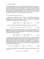
</div><span class="text_page_counter">Trang 7</span><div class="page_container" data-page="7"><b>CHAPTER II. KINEMATICS PROBLEM</b>
<b>2.1. Survey of forward kinematics</b>
<b>2.1.1. Setting coordinate system for robot</b>
Figure 1. Link-frame attachment
* Link-frame attachment procedure:
1. Identify the joint axes and imagine (or draw) infinite lines along them. For steps 2 through 5 below, consider two of these neighboring lines (at axes i and i ).1
2. Identify the common perpendicular between them, or point of intersection. At the point of intersection, or at the point where the common perpendicular meets the ith axis, assign the link-frame origin.
3. Assign the Z<sup>ˆ</sup><small>i</small>
axis pointing along the ith joint axis.
4. Assign the X<sup>ˆ</sup><small>i</small><sub> axis pointing along the common perpendicular, or, if the axes intersect, </sub>
assign X<sup>ˆ</sup><small>i</small><sub> to be normal to the plane containing the two axes.</sub>
5. Assign the Y<sup>ˆ</sup><small>i</small><sub> axis to complete a right-hand coordinate system.</sub>
6. Assign {0} to match {1} when the first joint variable is zero. For {N}, choose an
origin location and X<sup>ˆ</sup><small>N</small><sub> direction freely, but generally so as to cause as </sub>
linkage parameters as possible to become zero.
<b>2.1.2. Setting the Denavit-Hatenberg parameters</b>
- Use Denavit-Hartenberg (D-H) method to solve the forward kinematics problem.
</div><span class="text_page_counter">Trang 8</span><div class="page_container" data-page="8">- D-H Table:
Joint <small>i</small><sub></sub><small>1</small> a<sub>i</sub><sub></sub><sub>1</sub> d<small>i</small> <small>i</small>
1 <sub>0</sub> a<sub>0</sub> d<sub>1</sub> <sub>1</sub>2 <small>1</small> a<sub>1</sub> d<sub>2</sub> <sub>2</sub>
i <small>i</small><sub></sub><small>1</small> a<sub>i</sub><sub></sub><sub>1</sub> d<sub>i</sub> <sub>i</sub>where: a = the distance from <small>i</small> Z<sup>ˆ</sup><small>i</small><sub> to </sub><sub>Z</sub>ˆ<sub>i</sub><sub></sub><sub>1</sub>
<small>1</small>, <small>2</small> and <small>3</small> are joint variables.
<b>2.1.3. Coordinate transformation matrix</b>
- Transformation that transforms vectors defined in
i<small>0012211</small>. . . ... .<small>23i1</small>.<small>ii</small>T T T T <small>i</small> T T<small>i</small>
- The general form of this transformation:
0 0 0 1
R R R PR R R PT
R R RR R R RR R R
</div><span class="text_page_counter">Trang 9</span><div class="page_container" data-page="9"><small>i</small>PP<small>x</small> P<small>y</small> P<small>z</small> <sub>: is the postion vector.</sub>
<b>2.2. Forward kinematics problem</b>
cos sin 0sin cos 0 0
0 0 0 1aT
cos sin 0sin cos 0 0
0 0 0 1aT
cos sin 0sin cos 0 0
0 0 0 1aT
1 0 00 1 0 00 0 1 00 0 0 1
<small>0012</small>T<small>1</small>T T.<small>2</small>
cos sin 0 cossin cos 0 sin
aaT
</div><span class="text_page_counter">Trang 10</span><div class="page_container" data-page="10">+ Joint 3:
<small>0012023</small>T <small>1</small>T T T. .<small>23</small> <small>2</small>T T.<small>3</small>
<small>H</small>T T T T T<small>H</small> T T<small>H</small>
0, , ;cos ,cos ,cos ;sin ,sin ,sin ;cos c ,sin ;
c s 0 cs c 0 s s
L L cL LT
</div><span class="text_page_counter">Trang 11</span><div class="page_container" data-page="11">Figure 3a. Calculation of forward kinematics in MATLAB
Figure 3b. Tranformation matrix <sup>0</sup>T<sub> and </sub><small>0</small>
<small>H</small>T<sub> in MATLAB</sub>
<b>*** Calculation:a. Problem 2.2A</b>
</div><span class="text_page_counter">Trang 12</span><div class="page_container" data-page="12">0 1 0 01 0 0 5.50 0 1 00 0 0 1T
<small>H</small>T<sub> after subsituting given data of problem 2.2A</sub>
Figure 4b. Frame assignment of problem 2.2A
</div><span class="text_page_counter">Trang 13</span><div class="page_container" data-page="13">0 1 0 4.791 0 0 2.320 0 1 00 0 0 1T
Figure 5a. <sup>0</sup>T<sub> and </sub><small>0</small>
<small>H</small>T<sub> after subsituting given data of problem 2.2B</sub>
Figure 5b. Frame assignment of problem 2.2B
</div><span class="text_page_counter">Trang 14</span><div class="page_container" data-page="14">Figure 6a. <sup>0</sup>T<sub> and </sub><small>0</small>
<small>H</small>T<sub> after subsituting given data of problem 2.2C</sub>
Figure 6b. Frame assignment of problem 2.2C
11
</div><span class="text_page_counter">Trang 15</span><div class="page_container" data-page="15">- Assume
is given that:
c 00 0 1 00 0 0 1
<small>1 12 1231231 12 123 123</small>
c ,,
c ,s .c
s s
x L c L c Ly L s L s L
Find <small>1</small><sub>, </sub><sub>2</sub><sub> and </sub><sub>3</sub><sub>.</sub>
- Sovle the inverse kinematics problem+ We have 3 equations:
<small>1 12 1231231 12 123 123123</small>
c 1s 2 3x L c L c L
y L s L s L
+ Substituting
3 into
1and
2, we have two equations:
<small>31 12 1231 12 12</small>
4 5x L c L c L c
y L s L s L s
cos <sup>R</sup> , 1P Q <small></small> <sub></sub>
+ Substituting any one of these solutions back into
4 and
5gives us:
</div><span class="text_page_counter">Trang 16</span><div class="page_container" data-page="16"><small>1 112</small>
<small>2</small> <sub>1 1</sub> <sub>1 1</sub>
' 'Atan2 ,'
x L cc
L y L s x L c
<sub></sub>
+ Finally, <small>3</small><sub> can be determined from </sub>
3: <small>3</small> <small>1</small> <small>2</small><sub>.</sub>
- Conlcusion: From the inverse kinematics soltion for the 3-R manipulator, for a given end-effectorposition and orientation, there are two different ways of reaching it, each corresponding to a different value of <sub>. These different cofigurations are shown as below:</sub>
Figure 7. The two inverse kinematics solutions for the 3R manipulator:“elbow-up” configuration
1
and the “elbow-down” configuration
1
+ For : <sup>1</sup> <small>1</small>210.51<sup>0</sup><sub>Unsatisfied.</sub>+ For : 1 <small>1</small>90 ,<sup>0</sup><small>2</small>180 ,<sup>0</sup><small>3</small>360<sup>0</sup><sub>.</sub>
13
</div><span class="text_page_counter">Trang 17</span><div class="page_container" data-page="17">* Given: <small>0</small>
4.445, 4.664, 90 , 3.5 2 1.5x y L L L m* Result:
+ For : <sup>1</sup> <small>1</small>319.09<sup>0</sup><sub>Unsatisfied.</sub>+ For : 1 <small>000</small>
<small>1</small> 30 , <small>2</small> 45 , <small>3</small> 15 <sub>.</sub>
Figure 8a. Frame assignment of problem 2.3A
Figure 8b. Frame assignment of problem 2.3B
</div><span class="text_page_counter">Trang 18</span><div class="page_container" data-page="18"><b>CHAPTER III. STATICS</b>
<b>*** Calculation:</b>
* Given:
+ Initial joint angles:
<small>000123</small><sup>T</sup> 15 30 45 <sup>T</sup> + End-effector velocity: <small>0</small>
0, 2 0,3 0, 2
X<sup></sup> x y .+ Static force: <small>0</small>
<sup>T</sup>
1 2 3
<small>T</small> , ,
W f f m N N Nm.* Solutions:
Figure 9. Resolved-Rate-Algorithm block diagram
+ Use MATLAB to program and simulate Resolved-rate-control algorithm (simulate in 5 seconds, 0.1s for each step).
15
</div><span class="text_page_counter">Trang 19</span><div class="page_container" data-page="19">+ Graph 1. Joint rates (m/s)
</div><span class="text_page_counter">Trang 20</span><div class="page_container" data-page="20">+ Graph 2. Joint angles (rad)
+ Graph 3. X{ x y}<small>T</small>
m m rad
<sub> versus time</sub>17
</div><span class="text_page_counter">Trang 21</span><div class="page_container" data-page="21">+ Graph 4. Determinant of Jacobian matrix versus time
+ Graph 5. Joint torque T{ } <small>123T</small><sub> (Nm) versus time</sub>
</div><span class="text_page_counter">Trang 22</span><div class="page_container" data-page="22"><b>CHAPTER IV. MANIPULATOR DYNAMICS</b>
<b>4.1. The iterative Newton-Euler dynamics algorithm</b>
+ Outward iterations: : 0i 2
+ Inward iterations: : 3i 1
Figure 10. The force balance, including inertial forces, for a single manipulator link
20
</div><span class="text_page_counter">Trang 23</span><div class="page_container" data-page="23">- Use MATLAB to calculate
</div><span class="text_page_counter">Trang 24</span><div class="page_container" data-page="24">Figure 11a&b. Calculation of dynamics in MATLAB*Given:
+ Weight of each link: m<small>1</small> 20, m<small>2</small> 15, m<small>3</small> 10
kg+ Moment of inertia of each link:
<small>2</small>
<small>1</small> 0.5, <small>2</small> 0.2, <small>3</small> 0.1
I I I kgm+ Joint angles:
<small>000</small></div><span class="text_page_counter">Trang 25</span><div class="page_container" data-page="25"><b>CHAPTER V. CONCLUSION</b>
"Calculating and designing control problems for industrial robots" is a highly practical topic, whenthe industry is growing, competition is constantly demanding, productivity and quality must be improved thanks to modern machinery lines replacing manual labor of humans.
Thus, in the module "Designing a mechanical system - Robot", I learned how to calculate and design a control system for a robot. Specific work completed includes the following:
SCARA robot overview.
Calculating the forward kinematics, inverse kinematics. Calculating velocity, static forces.
Find out the dynamic problem of robot.
Through the above topic, I have learned how to apply professional knowledge trained at Hanoi University of Science and Technology in the past time into real life, especially with industry. I also learned a lot such as teamwork skills, problem solving, finding documents, writing reports... very useful for later. Once again, I would like to thank Dr. Tran Dinh Long helped me complete this thesis.
Due to the limitation of time and knowledge in this project, I only solved some fundamental problems in the design of a robot. In addition, there are many problems need to be solved to have a complete robot product such as mechanical design, equipment selection, algorithms, software programming, .... Therefore, I hope that other teachers and you will give me your comments to improve this topic.
Sincere thanks to all of you!
</div>