research and design of agv using slam ros system
Bạn đang xem bản rút gọn của tài liệu. Xem và tải ngay bản đầy đủ của tài liệu tại đây (5.88 MB, 88 trang )
<span class="text_page_counter">Trang 1</span><div class="page_container" data-page="1">
MINISTRY OF EDUCATION AND TRAINING
<b>HO CHI MINH CITY UNIVERSITY OF TECHNOLOGY AND EDUCATION FACULTY FOR HIGH QUALITY TRAINING </b>
<b> </b>
<b>GRADUATION PROJECT MANUFACTURING TECHNOLOGY</b>
</div><span class="text_page_counter">Trang 2</span><div class="page_container" data-page="2"><b>HO CHI MINH UNIVERSITY OF TECHNOLOGY AND EDUCATION </b>
<b>FACULTY OF INTERNATIONAL EDUCATION </b>
<b>GRADUATED PROJECT </b>
<b>RESEARCH AND DESIGN OF AGV USING SLAM (ROS) SYSTEM </b>
</div><span class="text_page_counter">Trang 3</span><div class="page_container" data-page="3"><b><small>TRƯỜNG ĐẠI HỌC SƯ PHẠM KỸ THUẬT CỘNG HÒA XÃ HỘI CHỦ NGHĨA VIỆT NAM </small></b>
<b>GRADUATION PROJECT TASK </b>
<b>Instructor: Dr. Vu Quang Huy Students: </b>
1. Nguyễn Văn Sơn ID: 19146116 Phone No: 0968823600 2. Trần Quốc Huy
<b>1. Project Number </b>
ID: 19146080 Phone No: 0898796821
<b>Name: Research, and design an AGV motor using SLAM (ROS) </b>
<b>2. Early figures and documents </b>
The AGV has the original specifications in dimensions of 281×281×156 (length × width × height). The material will be acrylic for the base and aluminum for the frames, it can carry up to 10kg with a maximum speed of 0,5 m/s, and the accuracy is expected to be about 80%.
<b>3. Main Project </b>
Investigate and construct an AGV truck that can operate in complicated termite warehouses. It has a 10 kg payload and is guided by a single LiDAR sensor. The Raspberry Pi 3 computer will get feedback from the LiDAR sensor once it has scanned the surrounding area. Based on such signals, a map will be created, which users may interact with to select their destination. The quickest route to the destination will then be determined by the AGV.
<b>4. Expected Project </b>
When the project is finished, an AGV will have the ability to scan and make a map, identify potential hazards ahead of time, and go as accurately as
</div><span class="text_page_counter">Trang 4</span><div class="page_container" data-page="4">have a display screen that allows users to communicate with them.
<b>5. Project delivery date </b>
<b>6. Project submission date </b>
</div><span class="text_page_counter">Trang 5</span><div class="page_container" data-page="5"><b>1.2. Introduction about AGV ... 4 </b>
<b>1.3. Structure of AGV system ... 7 </b>
<b>1.4. AGV application... 7 </b>
<b>1.5. Research nationally and internationally about AGV ... 10 </b>
<b>1.6. Object and scope of the study ... 12 </b>
<b>1.6.1. Object of the study ... 12 </b>
<b>1.6.2. Scope of the study ... 12 </b>
<b>1.7. Graduation project structure... 13 </b>
<b>CHAPTER 2: FUNDAMENTAL THEORY ... 14 </b>
<b>2.1. Robot’s Kinematics and Robot’s Dynamics ... 14 </b>
<b>2.1.1. Robot’s Kinematics ... 14 </b>
<b>2.1.2. Robot’s Dynamics ... 16 </b>
<b>2.2. SLAM TECHNOLOGY (Simultaneous Localization and Mapping) ... 18 </b>
<b>2.2.1. Mapping ... 18 </b>
<b>2.2.2. How SLAM works ... 19 </b>
<b>2.2.3. Common challenges with SLAM ... 23 </b>
<b>2.3. Path Planning with ROS ... 25 </b>
<b>CHAPTER 3: CALCULATION DESIGN ... 36 </b>
<b>3.1. Design requirements and transmission selection ... 36 </b>
</div><span class="text_page_counter">Trang 7</span><div class="page_container" data-page="7"><b>LIST OF FIGURES </b>
<i>Figure 1.1. Unit load AGV ... 5 </i>
<i>Figure 1.2. AGV forklifts ... 6 </i>
<i>Figure 1.3. Towing AGV ... 6 </i>
<i>Figure 1.4. AGV structure ... 7 </i>
<i>Figure 1.5. Manufacturing Industry AGV ... 8 </i>
<i>Figure 1.6. Warehousing and Distribution AGV ... 8 </i>
<i>Figure 1.7. Logistic and Supply Chain AGV ... 9 </i>
<i>Figure 1.8. Healthcare AGV ... 9 </i>
<i>Figure 1.9. Agriculture and Farming AGV ... 10 </i>
<i>Figure 1.10. Omron and KuKa AGV products ... 12 </i>
<i>Figure 2.1. Instantaneous Center of Curvature ... 14 </i>
<i>Figure 2.2. Robot Coordinate system ... 16 </i>
<i>Figure 2.3. Robot system model ... 17 </i>
<i>Figure 2.4. Benefits of SLAM for Cleaning Robots ... 19 </i>
<i>Figure 2.5. SLAM Processing Flow ... 20 </i>
<i>Figure 2.6. Structure from motion ... 21 </i>
<i>Figure 2.7. Point cloud registration for RGB-D SLAM ... 21 </i>
<i>Figure 2.8. SLAM in 2D Lidar ... 22 </i>
<i>Figure 2.9. SLAM in 3D Lidar ... 23 </i>
<i>Figure 2.10. Error localization ... 24 </i>
<i>Figure 2.11. Dynamic Window Approach ... 28 </i>
<i>Figure 2.12. DWA Algorithm Diagram ... 29 </i>
<i>Figure 2.13. Path Planning ... 30 </i>
<i>Figure 2.14. Feedback diagram ... 31 </i>
<i>Figure 2.15. PID controller graph ... 31 </i>
<i>Figure 2.16. PID controller function parameter ... 32 </i>
<i>Figure 2.17. Belt drive ... 33 </i>
<i>Figure 2.18. Chain Drive ... 34 </i>
<i>Figure 2.19. Gear drive ... 35 </i>
<i>Figure 3.1. AGV mechanical options ... 37 </i>
<i>Figure 3.2. Active wheel ... 38 </i>
<i>Figure 3.3. Guide wheels ... 38 </i>
<i>Figure 3.4. Basement mechanical ... 40 </i>
<i>Figure 3.5. Design mechanical ... 41 </i>
<i>Figure 3.6. Stress simulation ... 42 </i>
<i>Figure 3.7. Force acting ... 46 </i>
<i>Figure 3.8. Operation diagram ... 48 </i>
<i>Figure 3.9. Electrical schematic ... 49 </i>
<i>Figure 3.10. Manual mode ... 50 </i>
<i>Figure 3.11. Automation mode ... 51 </i>
</div><span class="text_page_counter">Trang 8</span><div class="page_container" data-page="8"><i>Figure 4.3. MPU 6050 ... 56 </i>
<i>Figure 4.4. Principle diagram MPU 6050 ... 57 </i>
<i>Figure 4.5. Arduino Mega 2560 ... 57 </i>
<i>Figure 4.6. RPLidar dimension ... 58 </i>
<i>Figure 4.7. Install control unit & transmission system ... 59 </i>
<i>Figure 4.8. Completed mobile robot ... 60 </i>
<i>Figure 4.9. Grid map method ... 61 </i>
<i>Figure 4.10. Setup the environment ... 61 </i>
<i>Figure 4.11. Choose a target position on the map ... 62 </i>
<i>Figure 4.12. Move from a position to another - mark with black tape ... 62 </i>
<i>Figure 4.13. Result Experiment 1 in bar chart ... 64 </i>
<i>Figure 4.14. The second experiment - moving U shape ... 65 </i>
<i>Figure 4.15. Result Experiment 2 in bar chart ... 66 </i>
<i>Figure 4.16. Check the detection of obstacles ... 67 </i>
<i>Figure 4.17. The mobile robot changes the route when encounter the obstacle ... 68 </i>
<i>Figure 4.18. Describe picture in the map and reality ... 68 </i>
</div><span class="text_page_counter">Trang 9</span><div class="page_container" data-page="9"><b>LIST OF TABLES </b>
<i>Table 1. Design requirement ... 36 </i>
<i>Table 2. AGV options ... 37 </i>
<i>Table 3. Comparison transmitter ... 39 </i>
<i>Table 4. Calculation parameter ... 46 </i>
<i>Table 5. Force parameter ... 46 </i>
<i>Table 6. Raspberry Bi 4 specifications ... 54 </i>
<i>Table 7. RPLidar parameter ... 58 </i>
<i>Table 8. Experiment 1 result ... 63 </i>
<i>Table 9. Describes Experiment 2 - Deviation of starting position and destination ... 65 </i>
</div><span class="text_page_counter">Trang 10</span><div class="page_container" data-page="10"><b>ABSTRACT </b>
Our country is becoming more and more modernized and industrialized. Compared with other powers to catch up with them in development, our country's industry needs to have access to modern technologies and equipment. Technology engineers need to be equipped with broader and new knowledge to be able to meet the needs of accelerating the country's development. Robot engineering technology has been and will be widely applied in many countries. It brings us many benefits in terms of productivity, and high job efficiency in many fields such as industrial production, medicine, society, space exploration, etc. However, in the robotics industry In our country, the scale is quite large, but the quality is not high due to limitations in science and technology, machinery and equipment are still rudimentary, so labor productivity is only average. An automated guided vehicle is the most famous robot used in foreign companies to transport automatic products. We are going to search and do this project to figure out the information about this robot, which can improve our skills and have an overview of the engineer.
The scientific significance of the topic:
Bringing lots of advances in the application of modern science and technology to the production process, which is the basis for building automated processes with the best equipment and machines. In addition, it can also show that students' understanding is increasingly enhanced when they have mastered the basic knowledge of science and creatively and effectively apply it to life.
<i>Keywords: AGV, Automated Guided Vehicle, IR sensor, Ultrasonic sensor, Arduino… </i>
</div><span class="text_page_counter">Trang 11</span><div class="page_container" data-page="11"><b>THESIS ACKNOWLEDGMENT </b>
We would like to express our deepest appreciation to our esteemed advisor, Mr. Vu Quang Huy, for his invaluable guidance and support throughout the completion of this report. His wisdom and expertise have been crucial in steering us in the right direction, ensuring our focus and dedication until the culmination of our efforts.
To our close companions who have accompanied us on this transformative four- year university journey, we owe a debt of gratitude. Amidst the challenges of student life, you have been our pillars of strength, offering assistance when needed and sharing in our triumphs and struggles. In times of difficulty, the strong bonds of friendship have illuminated our path and rejuvenated our spirits.
We are profoundly grateful to our beloved parents and cherished loved ones for their unwavering support, continuous encouragement, and steadfast belief in our abilities. Their presence has provided us with the strength and determination to see this project through to completion. Their love and encouragement have been the driving force behind our endeavors, and we are forever thankful for their unwavering faith in us.
Additionally, we extend our thanks to Ho Chi Minh City University of Technology and Education and the Faculty of High-Quality Training for providing us with the necessary resources and support to undertake our graduation project.
In conclusion, we wish to convey our deepest gratitude to our parents, loved ones, friends, advisors, and our university for their unwavering support, guidance, and contributions to our academic journey. Without their presence and influence, our success and personal growth would not have been possible. Their contributions have been invaluable, and we will always cherish the profound impact they have had on our lives.
</div><span class="text_page_counter">Trang 12</span><div class="page_container" data-page="12"><b>CHAPTER 1: INTRODUCTION </b>
<b>1.1. History </b>
The history of Automation Guide Vehicles (AGVs) traces back to the mid-20th century, with the development of early automated material handling systems. Here's a brief overview of key milestones in the history of AGVs:
1950s: The concept of AGVs began to emerge in the 1950s, primarily driven by the need for automation in manufacturing and material handling industries. Early AGVs were simple vehicles guided by wires embedded in the floor or by magnetic tape.
1960s: AGV technology continued to evolve in the 1960s, with the introduction of more sophisticated guidance systems such as radio frequency (RF) and optical navigation. These advancements enable AGVs to navigate more complex environments and perform a wider range of tasks in industrial settings.
1970s: The 1970s saw further advancements in AGV technology, including the development of onboard computers and sensors for obstacle detection and navigation. AGVs began to gain traction in industries such as automotive manufacturing, where they were used for parts delivery and assembly line logistics.
1980s: During the 1980s, AGVs became more widespread in industries such as warehousing, distribution, and logistics. The introduction of laser guidance systems allows AGVs to navigate without the need for physical infrastructure like wires or tapes, making them more flexible and adaptable to changing environments.
1990s: In the 1990s, AGV technology continued to mature, with improvements in sensors, software, and communication systems. AGVs became more integrated with other automation technologies such as robotics and warehouse management systems, enabling seamless operation in complex industrial environments.
2000s: The 21st century brought significant advancements in AGV capabilities, driven by innovations in artificial intelligence, machine learning, and sensor technology. AGVs became smarter, more agile, and more autonomous, capable of performing a wide range of tasks with minimal human intervention.
</div><span class="text_page_counter">Trang 13</span><div class="page_container" data-page="13">2010s and Beyond: In recent years, AGVs have seen widespread adoption across various industries worldwide, driven by the need for increased efficiency, productivity, and safety. Today's AGVs are equipped with advanced features such as real-time data analytics, predictive maintenance, and collaborative robotics, enabling them to revolutionize the way goods are transported and managed in the digital age.
Overall, the history of AGVs reflects a trajectory of continuous innovation and technological advancement, with these vehicles evolving from simple guided carts to sophisticated autonomous systems that are reshaping the future of transportation, logistics, and manufacturing.
<b>1.2. Introduction about AGV </b>
An automatic guided vehicle system (AGVS) consists of one or more computer- controlled, wheel-based load carriers (normally battery-powered) that run on the plant or warehouse floor (or outdoors on a paved area) without the need for an onboard operator or driver. (MHI)
An automated guided vehicle or automatic guided vehicle (AGV) is a mobile robot that follows markers or wires in the floor or uses vision or lasers. They are most often used in industrial applications to move materials around a manufacturing facility or a warehouse.
The term "automated guided vehicle" (AGV) is a general one that encompasses all transport systems capable of functioning without driver operation. The term "driverless" is often used in the context of automatic guided vehicles to describe industrial trucks, used primarily in manufacturing and distribution settings, that would conventionally have been driver-operated
A materials handling system that uses automated vehicles such as carts, pallets or trays which are programmed to move between different manufacturing and warehouse stations without a driver. These systems are used to increase efficiency, decrease damage to goods and reduce overhead by limiting the number of employees required to complete the job.
</div><span class="text_page_counter">Trang 14</span><div class="page_container" data-page="14">Each type of goods has different requirements when storing and transporting, so there are multiple shipping methods. In the factory, there are usually 3 types of AGV, this type of AGV covers most transportation jobs.
• Unit load AGV vehicles
In simple terms, these robots are portable and autonomous cargo delivery systems that are able to travel around a warehouse or facilities performing different AGV navigation technologies. These fascinating robots are mainly used for industrial transport of goods and heavy materials around warehouses or storage facilities.
A unit load AGV is a powered, wheel based transport vehicle that carries a discrete load, such as an individual item or items contained on a pallet or in a tote or similar temporary storage medium.
<i>Figure 1.1. Unit load AGV </i>
• AGV forklifts
An Automatic Guided Forklift also known as ALT is a Self-Driving computer- controlled Forklift. So a forklift moving around and transporting goods by its own without human intervention, it's just a driverless forklift. It is the typical automated guided vehicle (agv) with forks. The automated forklift trucks are increasingly becoming a must in manufacturing premises and warehouses where operations are highly standardized, repetitive, and easily accomplished without need of human intervention. Forklift robots are widely used in warehouses for high rack management.
</div><span class="text_page_counter">Trang 15</span><div class="page_container" data-page="15"><i>Figure 1.2. AGV forklifts </i>
• Towing (or tugger) AGV
Towing vehicles, or tugger automatic guided vehicles, pull one or more non- powered, load-carrying vehicles behind them in a train-like formation. Sometimes called driverless trains, powered towing vehicles travel on wheels. Tugger automatic guided vehicles are often used for transporting heavy loads over longer distances. They may have several drop-off and pick-up stops along a defined path through a warehouse or factory.
<i>Figure 1.3. Towing AGV </i>
</div><span class="text_page_counter">Trang 16</span><div class="page_container" data-page="16"><b>1.3. Structure of AGV system </b>
<i>Figure 1.4. AGV structure </i>
<b>1.4. AGV application </b>
Automation Guide Vehicles (AGVs) have found application in various industries around the world, revolutionizing traditional methods of transportation, logistics, and manufacturing. Here are some notable applications of AGVs across different sector.
Manufacturing Industry: AGVs are extensively used in manufacturing plants for material handling, parts delivery, and assembly line operations. These vehicles transport raw materials and components between workstations, increase efficiency and reduce the need for manual labor. AGVs also facilitate just-in-time manufacturing processes, optimizing production schedules and minimizing inventory storage costs.
</div><span class="text_page_counter">Trang 17</span><div class="page_container" data-page="17"><i>Figure 1.5. Manufacturing Industry AGV </i>
Warehousing and Distribution Centers: AGVs play a crucial role in modern warehouses and distribution centers by automating inventory management, order picking, and goods transportation. They navigate through aisles, locate items, and transport them to designated locations with precision and efficiency. AGVs enable warehouses to operate around the clock, speeding up order fulfillment and reducing labor costs.
<i>Figure 1.6. Warehousing and Distribution AGV </i>
Logistics and Supply Chain Management: In the logistics industry, AGVs streamline the movement of goods within warehouses, ports, and transportation hubs. These vehicles are equipped with advanced navigation systems that enable them to navigate complex environments, avoid obstacles, and optimize route planning. AGVs enhance supply chain efficiency by minimizing transit times, reducing errors, and
</div><span class="text_page_counter">Trang 18</span><div class="page_container" data-page="18"><i>Figure 1.7. Logistic and Supply Chain AGV </i>
Healthcare Facilities: AGVs are increasingly being deployed in hospitals and healthcare facilities to automate the delivery of medications, medical supplies, and equipment. These vehicles transport items between different departments, such as pharmacy, laboratories, and patient rooms, while adhering to strict hygiene and safety protocols. AGVs help healthcare providers streamline operations, reduce human errors, and improve patient care.
<i>Figure 1.8. Healthcare AGV </i>
Agriculture and Farming: AGVs are starting to find applications in agriculture for tasks such as crop monitoring, harvesting, and transportation. These vehicles can navigate fields autonomously, identify ripe crops, and collect produce without the need
</div><span class="text_page_counter">Trang 19</span><div class="page_container" data-page="19">for human intervention. AGVs have the potential to revolutionize farming practices by increasing efficiency, reducing labor costs, and minimizing environmental impact.
<i>Figure 1.9. Agriculture and Farming AGV </i>
Overall, Automation Guide Vehicles have become indispensable tools for enhancing efficiency, productivity, and safety across various industries worldwide. As technology continues to advance, we can expect AGVs to play an even greater role in reshaping the future of transportation and logistics.
<b>1.5. Research nationally and internationally about AGV </b>
• International - Post pandemic world
During the epidemic, the globe has seen a tremendous increase in autonomous mobile robots. As the globe prepares to reconnect in the post-pandemic era, autonomous mobile robots will play a role in industry, hospitality, and healthcare. Automation has become more important in the retail, manufacturing, warehouse, and restaurant industries. Automation has introduced varying degrees of autonomy into the picture.
For example, in factories, autonomous mobile robots have taken over labor-intensive operations such as picking, sorting, and transporting. These robots handle millions of components without the need for human intervention, enhancing material flow.
In healthcare, robots can assist with duties such as cleaning and sterilization, medicine, food, and garbage distribution, and others when human presence is not required.
</div><span class="text_page_counter">Trang 20</span><div class="page_container" data-page="20">• National - In Viet Nam
The field of mobile robots with many navigation sensors and cameras is being studied by many domestic units. Issues of high-speed image processing, multi-sensor coordination, spatial positioning and mapping, orbital motion design avoiding obstructions for mobile robots have been published in the National Mechatronics conferences in 2002, 2004, 2006, 2008 and 2010. Robotic Vision studies are of interest both in industrial robots and mobile robots, particularly in the field of robotic identification and control on the basis of visual information.
Along with the construction of robots, the published scientific research on robots by Vietnamese scientists is very diverse and closely follows the research directions of the world. Robotics studies in Vietnam are heavily involved in issues of kinetics, dynamics, orbital design, sensor information processing, actuation, control and intelligence development for robots. Studies in robotic kinetics and dynamics are of interest both in the civil and military faculties of mechanics, machine-building at universities and research institutes in mechanics and machine-building.
A few famous companies that manufacturing AGV, AMR in Viet Nam can be mentioned as:
o Robot AGV Perbot Uniduc: Uniduc has successfully designed and applied AGV robotic systems in factories across the country. This is also considered as one of the strengths of the company, with a variety of products with low to high loads, diverse design.
o AGV Yaskawa: since 2010 with 2 main products are towing rows and roaring robots. Has an average load of 500kg speed of 10m/min.
o KuKa Group: more than 40 years of experience in the field of automation; in the production of AGV robots the company promotes product diversity.
o AGV Omron: With over 40 years of experience. Omron's AGV has a wide selection of products loading from >500 kg which is quite large. Speed 0.5, / s. Battery selectable for model charging time 6h/8h/10h. The clock and HMI display have a convenient button.
</div><span class="text_page_counter">Trang 21</span><div class="page_container" data-page="21"><i>Figure 1.10. Omron and KuKa AGV products </i>
<b>1.6. Object and scope of the study </b>
<b>1.6.1. Object of the study </b>
Research on Automation Guide Vehicles (AGVs) in the field of freight transport is an area that is attracting the attention of researchers and freight experts around the world. In this study, AGVs were surveyed and analyzed to understand the features, performance, and applications of each type in the freight transport process.
Common types of AGVs in research include AGVs with sensor-guided positioning, self-guided AGVs with GPS, self-guided AGVs with laser scanners, and self-guided AGVs with cameras. Each of these types of AGVs has its own advantages and limitations, and this study focuses on comparing and evaluating them to select the type of vehicle that best suits the specific requirements of each cargo transport process.
The goal of this research is to provide detailed information and accurate analysis of AGVs for decision support in deploying and optimizing freight transportation systems. By clearly understanding the advantages and disadvantages of each type of AGVs and applying them in specific freight transport environments, this research contributes to improving the efficiency and effectiveness of the freight transport process, while creating theoretical basis for the further development of AGVs technology in this field.
<b>1.6.2. Scope of the study </b>
Transporting large amounts of heavy products from one location to another will no longer be an issue with the assistance of an AGV. The robot will be in charge of
</div><span class="text_page_counter">Trang 22</span><div class="page_container" data-page="22">autonomously transporting big boxes across a large facility such as a warehouse or factory.
Using Lidar technology, a way to measure distance by continuously emitted lasers to objects and recording the laser's response time to the receiver. Once Lidar has completed the ambient scan, it sends data back to the computer using ROS to set up a map of the surrounding area and save it in the library. We will also mark specific destinations on the map and save it.
Then, just by selecting destinations that are already stored on the computer, ROS will provide the appropriate route to guide and send a signal to the raspberry to start the encoder engines are being controlled and the robot will begin to move to the destination.
<b>1.7. Graduation project structure </b>
This graduation project is divided into six sections, each of which has the following specific contents:
Chapter 1: INTRODUCTION - In this chapter our team present an overview of AGVs (Automation Guide Vehicles) and detail the research object and objectives of the report. It will gain a foundational understanding of AGVs and the specific focus of the research conducted in the report. That can expect to learn and explore in the subsequent sections of the chapter. Overall, it serves as a roadmap for the chapter's content, guiding readers through the key topics and objectives to be covered.
Chapter 2: FUNDAMENTAL THEORY - This chapter presents for the relevant theories and the applications to the topic.
Chapter 3: CALCULATION DESIGN - This chapter presents for the method for choosing equipments and desgin the product.
Chapter 4: IMPLEMENT, EXPERIMENT AND RESULT ANALYSES - This chapter presents starting the programme, collects the result number then evaluation.
Chapter 5: CONCLUSION - This chapter is the summary of the topic and shows the product development directions in the future.
</div><span class="text_page_counter">Trang 23</span><div class="page_container" data-page="23"><b>CHAPTER 2: FUNDAMENTAL THEORY </b>
<b>2.1. Robot’s Kinematics and Robot’s Dynamics </b>
<b>2.1.1. Robot’s Kinematics </b>
Differential drive, often known as independent steering, is the driving system used by mobile robots. The number of the robot's propulsion wheels determines how this system operates. This mechanism typically comprises two wheels mounted on a single axle. Each wheel includes a driving wheel to prevent the robot from overturning and may be moved separately forward or backward. We can turn the robot left or right by varying the velocity of a wheel. Additionally, the robot will revolve around an object on either side of the wheel axle. The Instantaneous Center of Curvature, or ICC, is the name given to that place in space.
<i>Figure 2.1. Instantaneous Center of Curvature </i>
When we change the speed of the two wheels, we will change the robot's trajectory.
Since the angular speed around the ICC at 2 wheels is the same, we can write:
𝜔
∗ (𝑅 + <sup>𝑙 </sup>) = 𝑉<sub>𝑟 </sub> (1)<small>2 </small>
</div><span class="text_page_counter">Trang 24</span><div class="page_container" data-page="24">l: distance hold 2 wheels.
𝑅: distance from ICC to the midpoint between 2 wheels. 𝑉<small>𝑟 </small>: is the right wheel velocity & 𝑉<small>𝑙 </small>is the left wheel velocity.
ω
: is the angular velocity around the ICC. → We have:We have 3 cases for this model as follows:
• 𝑉<sub>𝑟 </sub>= 𝑉<sub>𝑙</sub>: the robot moves in a straight line linearly. 𝑅 is infinite and 𝜔 = 0
• 𝑉<sub>𝑟 </sub>= - 𝑉<sub>𝑙 </sub>: 𝑅 = 0: robots rotate around the wheel axle midpoint – robots rotate in place.
• 𝑉<sub>𝑟 </sub> = 0: The robot rotates towards the right wheel, now <sup>1 </sup>Similarly, for 𝑉<small>𝑙 </small>=
</div><span class="text_page_counter">Trang 25</span><div class="page_container" data-page="25">The robot's system model is depicted in the figure below, where r is the wheel radius and L is the distance between two wheels. This model has two limitations: Monday is a non-vertical sliding robot, and there is no side sliding between two active wheels and the ground. The following equation describes these two constraints:
𝑥<sub>𝑐 </sub>x cos(cos 𝛳) - 𝑦<sub>𝑐 </sub> x sin(sin𝛳) = 0 (8) 𝑥<sub>𝑐 </sub>x cos(cos 𝛳) - 𝑦<sub>𝑐 </sub> x sin(sin𝛳) = <sup>𝑟 </sup>x ( 𝜑<sub>𝑟 </sub>+𝜑<sub>𝑙 </sub>) (9)
In which, (𝑥𝑐, 𝑦𝑐) is the coordinates of the robot's center, 𝜃 is the angle between the robot's x axis and the global x axis, 𝜑𝑟, 𝜑𝑙 is the angle position of the cake on the right and the cake on the left.
</div><span class="text_page_counter">Trang 26</span><div class="page_container" data-page="26"><i>Figure 2.3. Robot system model </i>
Robot dynamics equations:
𝑀(𝑞)𝑞 + 𝐶(𝑞) + 𝐺(𝑞) + 𝜏<small>𝑑 </small>= 𝐵(𝑞)𝜏 + 𝐴<small>𝑇</small>(𝑞)𝜏 (10) Where M (q) is inertia, is the matrix containing the terms centrifugal and Coriolis
G(q) is the gravity matrix B(q) is the input variable matrix
τ is the input moment s the gravity matrix B(q) is the input variable matrix
𝐴𝑇(q) is the Jacobian matrix associated with constraints λ is the binding force vector
q is the state vector representing the general coordinates 𝜏𝑑 denotes unclear external perturbations.
𝑀(𝑞) = [𝑚 0 0 0 𝑚 0 0 0 𝐼] (11) 𝐴<small>𝑇</small>(𝑞) = [𝜃 𝑐𝑜𝑠 𝑐𝑜𝑠 𝜃 0] (12)
</div><span class="text_page_counter">Trang 27</span><div class="page_container" data-page="27">For example, imagine a household robot vacuum cleaner. Without SLAM, it moves randomly around the room and may not be able to clean the entire floor surface. This method also uses a lot of power, which drains your battery faster. Robots using SLAM, on the other hand, can use information such as wheel rotation speed and data from image sensors such as cameras to calculate the amount of movement required. This is called localization. The robot can also use cameras and other sensors simultaneously to create a map of obstacles around it to avoid repeatedly cleaning the same area. This is called mapping.
</div><span class="text_page_counter">Trang 28</span><div class="page_container" data-page="28"><i>Figure 2.4. Benefits of SLAM for Cleaning Robots </i>
SLAM is useful in many other applications such as navigating a fleet of mobile robots to arrange shelves in a warehouse, parking a self-driving car in an empty spot, or delivering a package by navigating a drone in an unknown environment. MATLAB and Simulink provide SLAM algorithms, functions, and analysis tools to develop various applications. You can implement simultaneous localization and mapping along with other tasks such as sensor fusion, object tracking, path planning, and path following.
<b>2.2.2. How SLAM works </b>
SLAM works by combining data from multiple sensors to create a map of an environment and to determine the robot’s location within that map. The sensors used can vary depending on the type of robot and the environment it’s navigating through. For example, a robot navigating through an indoor environment might use cameras and lidar, while a robot navigating through an outdoor environment might use GPS and sonar.
The data collected by the sensors is processed and combined using algorithms that create a map of the environment and determine the robot’s location within that map. This process is complex and requires a high degree of computational power, but recent advances in machine learning and artificial intelligence have made it easier and more efficient.
Broadly speaking, there are two types of technology components used to achieve SLAM. The first type is sensor signal processing, including front-end processing, which
</div><span class="text_page_counter">Trang 29</span><div class="page_container" data-page="29">is largely dependent on the sensors used. The second type is pose-graph optimization, including the back-end processing, which is sensor-agnostic.
<i>Figure 2.5. SLAM Processing Flow 2.2.2.1. Visual SLAM </i>
As the name suggests, visual SLAM (or vSLAM) uses images acquired from cameras and other image sensors. Visual SLAM can use simple cameras (wide angle, fish-eye, and spherical cameras), compound eye cameras (stereo and multi cameras), and RGB-D cameras (depth and ToF cameras).
Visual SLAM can be implemented at low cost with relatively inexpensive cameras. In addition, since cameras provide a large volume of information, they can be used to detect landmarks (previously measured positions). Landmark detection can also be combined with graph-based optimization, achieving flexibility in SLAM implementation.
Monocular SLAM is when vSLAM uses a single camera as the only sensor, which makes it challenging to define depth. This can be solved by either detecting AR markers, checkerboards, or other known objects in the image for localization or by fusing the camera information with another sensor such as inertial measurement units (IMUs), which can measure physical quantities such as velocity and orientation. Technology related to vSLAM includes structure from motion (SfM), visual odometry, and bundle adjustment.
Visual SLAM algorithms can be broadly classified into two categories. Sparse
</div><span class="text_page_counter">Trang 30</span><div class="page_container" data-page="30">SLAM. Dense methods use the overall brightness of images and use algorithms such as DTAM, LSD-SLAM, DSO, and SVO.
<i>Figure 2.6. Structure from motion </i>
<i>Figure 2.7. Point cloud registration for RGB-D SLAM 2.2.2.2. Lidar SLAM </i>
Light detection and ranging (lidar) is a method that primarily uses a laser sensor (or distance sensor).
Compared to cameras, ToF, and other sensors, lasers are significantly more precise and are used for applications with high-speed moving vehicles such as self- driving cars and drones. The output values from laser sensors are generally 2D (x, y) or
</div><span class="text_page_counter">Trang 31</span><div class="page_container" data-page="31">3D (x, y, z) point cloud data. The laser sensor point cloud provides high-precision distance measurements and works very effectively for map construction with SLAM. Generally, movement is estimated sequentially by matching the point clouds. The calculated movement (traveled distance) is used for localizing the vehicle. For lidar point cloud matching, registration algorithms such as iterative closest point (ICP) and normal distributions transform (NDT) algorithms are used. 2D or 3D point cloud maps can be represented as a grid map or voxel map.
On the other hand, point clouds are not as finely detailed as images in terms of density and do not always provide sufficient features for matching. For example, in places where there are few obstacles, it is difficult to align the point clouds and this may result in losing track of the vehicle's location. In addition, point cloud matching generally requires high processing power, so it is necessary to optimize the processes to improve speed. Due to these challenges, localization for autonomous vehicles may involve fusing other measurement results such as wheel odometry, global navigation satellite system (GNSS), and IMU data. For applications such as warehouse robots, 2D lidar SLAM is commonly used, whereas SLAM using 3-D lidar point clouds can be used for UAVs and automated driving.
<i>Figure 2.8. SLAM in 2D Lidar </i>
</div><span class="text_page_counter">Trang 32</span><div class="page_container" data-page="32"><i>Figure 2.9. SLAM in 3D Lidar </i>
<b>2.2.3. Common challenges with SLAM </b>
Although SLAM is used for some practical applications, several technical challenges prevent more general-purpose adoption. Each has a countermeasure that can help overcome the obstacle.
• Localization errors accumulate, causing substantial deviation from actual values
SLAM estimates continuous motion, which is subject to some degree of error. Errors accumulate over time and lead to significant deviations from the actual value. Additionally, map data may become corrupted or distorted, making further exploration difficult. Taking care of the case of driving along a square aisle as an example. As errors accumulate, the robot's start and end points will no longer match. This is called the loop closure problem.
It is important to be aware of loop closures and determine how to correct or cancel the accumulated errors. The solution is to remember some features of previously visited places as landmarks to minimize the localization error. Pose diagrams are created to correct errors. By solving error minimization as an optimization problem, more accurate map data can be generated. This type of optimization is called bundle adjustment in Visual SLAM.
</div><span class="text_page_counter">Trang 33</span><div class="page_container" data-page="33"><i>Figure 2.10. Error localization </i>
• Localization fails and the position on the map
Imagery and point cloud mapping do not take into account the robot's motion characteristics. In some cases, this approach can produce discontinuous position estimates.
This type of localization error can be prevented by using recovery algorithms or by fusing the motion model with multiple sensors and performing computations based on sensor data. There are several ways to use motion models with sensor fusion.
A common method is to use Kalman filtering for localization. In general, many differential drive robots and four-wheeled vehicles use nonlinear motion models, so advanced Kalman filters and particle filters (Monte Carlo localization) are often used. Commonly used sensors include IMUs, attitude heading reference systems (AHRS), inertial navigation systems (INS), and inertial measurement devices such as accelerometers, gyro sensors, and magnetic sensors. Automotive wheel encoders are often used to measure mileage.
A recovery measure, if localization fails, is to remember landmarks as keyframes
</div><span class="text_page_counter">Trang 34</span><div class="page_container" data-page="34">processing is applied to scan at high speed. Some image feature-based methods include feature bags and visual word bags. Recently, deep learning has been used to compare distances of features.
• High computational cost for image processing, point cloud processing, and optimization
Computing cost is a problem when implementing SLAM on-vehicle hardware. Computation is usually performed on compact and low-energy embedded microprocessors that have limited processing power. To achieve accurate localization, it is essential to execute image processing and point cloud matching at high frequency. In addition, optimization calculations such as loop closure are high computation processes. The challenge is how to execute such computationally expensive processing on embedded microcomputers.
One countermeasure is to run different processes in parallel. Processes such as feature extraction, which is the preprocessing of the matching process, are relatively suitable for parallelization. Using multicore CPUs for processing, single instruction multiple data (SIMD) calculation and embedded GPUs can further improve speeds in some cases. Also, since pose graph optimization can be performed over a relatively long cycle, lowering its priority and carrying out this process at regular intervals can also improve performance.
<b>2.3. Path Planning with ROS </b>
<b>2.3.1. Definition of ROS </b>
This project uses ROS to control LiDAR sensors, scan and map the environment, and set fixed targets to create closed working routes for AGVs. ROS is installed on a personal laptop with the main operating system Ubuntu and connected to LiDAR (map scanning) and Arduino (motor control).
ROS (Robot Operating System) is an open-source framework that helps researchers and developers build and reuse code between robotic applications. It is also a set of tools, libraries, and protocols designed to make it easier to create complicated and resilient robot behavior across a wide range of automated systems.
</div><span class="text_page_counter">Trang 35</span><div class="page_container" data-page="35">ROS is a software package that enables the rapid and easy development of autonomous robotic systems. ROS should be viewed as a set of tools for developing new solutions or modifying old ones. This system has many drivers and developed algorithms that are frequently used in automation robots. Components of the ROS system include
<b>Nodes: which represent one process running the ROS graph. Nodes oversee the </b>
management of devices or computing technology, and each node performs specific tasks. Topics or services can be used for communication between nodes. ROS software comes packaged. A single package is typically created to perform a single type of operation and can span one or more nodes.
<b>Topics: In ROS, topics are streams of data that nodes use to exchange </b>
information. These are used to send repeated messages of the same type. This can be a sensor reading or motor speed.
Each subject is registered with a unique name and message type. Nodes can connect to it to publish or subscribe to messages. A node cannot publish and subscribe to a particular topic at the same time, but there is no limit to the number of different nodes that can publish or subscribe to that topic.
<b>Services: Service communication is similar to a client/server approach. In this </b>
configuration, nodes (servers) register services with the system. Other nodes can then request this service and receive responses. Unlike topics, services can also include data in requests, allowing two-way communication.
<b>Parameter server: A parameter server is a database shared between nodes that </b>
allows shared access to static or semi-static information. Data that does not change frequently and is accessed infrequently, such as the distance between her two fixed points in the environment or the weight of the robot, is a good candidate to store in a parameter server.
<b>2.3.2. Navigation Method </b>
Path planning for a mobile robot involves determining the sequence of operations
</div><span class="text_page_counter">Trang 36</span><div class="page_container" data-page="36">collisions with objects. Path planning algorithms include Dijkstra's algorithm, A* or A- star, D* or dynamic A*, artificial potential field methods, and visibility graph methods. Path planning algorithms can be based on graphs or occupancy grids.
Diagram-based methods show where the robot is and how it can move between different locations. In this format, vertices represent locations, such as rooms in a building, and edges define paths between vertices, such as doors that connect rooms.
Additionally, each edge can be assigned a weight that indicates the complexity of the travel path, such as the width of the door or the energy required to open it. The trajectory is determined by determining the shortest path between two vertices. One of the vertices is the robot's current position and the other is the target.
<b>2.4. Dynamic Window Approach (DWA) </b>
The Dynamic Window Approach (DWA)’s method works following the principle:
1. Discretely test within the robot's control space (dx,dy,dtheta)
2. For each inspected speed, perform a forward reenactment from the robot's current state to foresee what would happen on the off chance that the inspected speed was connected for a few (brief) period of time.
3. Assess (score) each direction coming about from the forward reenactment, employing a metric that joins characteristics such as nearness to deterrents, nearness to the objective, vicinity to the worldwide way, and speed. Dispose of unlawful directions (those that collide with obstacles).
4. Choose the highest-scoring direction and send the related speed to the versatile base.
5. Risen and repeat.
</div><span class="text_page_counter">Trang 37</span><div class="page_container" data-page="37"><i>Figure 2.11. Dynamic Window Approach </i>
The goal of DWA is to produce a (v, ω) pair which represents a circular trajectory that is optimal for robot’s local condition. DWA reaches this goal by searching the velocity space in the next time interval. The velocities in this space are restricted to be admissible,which means the robot must be able to stop before reaching the closest obstacle on the circular trajectory dictated by these admissible velocities. Also, DWA will only consider velocities within a dynamic window, which is defined to be the set of velocity pairs that is reachable within the next time interval given the current translational and rotational velocities and accelerations.
The Energetic Window Approach has two essential objectives: to compute a substantial speed look space and to select the finest speed. The look space is built from the set of speeds that result in a secure direction (i.e., empower the robot to halt some time recently colliding), given the set of velocities that the robot can accomplish within the following time cut given its elements ('dynamic window'). The perfect speed is utilized to optimize the robot's clearance, velocity, and heading closest to the target.
So in DWA we are going have a few basic step to discover the most excellent speed to make direction for our robot:
</div><span class="text_page_counter">Trang 38</span><div class="page_container" data-page="38"><i>Figure 2.12. DWA Algorithm Diagram </i>
1. To begin with, depending on our show position and the target, we may compute the required speed to the objective. (For case, in case we are distant absent, travel quickly; in the event that we are near, go gradually).
2. Given the vehicle elements, select the passable speeds (direct 'v' and precise 'w'). 3. Go through all of the conceivable speeds.
4. Decide the closest deterrent for the arranged robot speed for each speed (i.e., collision discovery along the direction) for each speed.
</div><span class="text_page_counter">Trang 39</span><div class="page_container" data-page="39">5. Decide in the event that the remove between the robot and the closest impediment is inside the robot's breaking distance. In case the robot cannot halt in time, dispose of the proposed robot speed.
6. In case the speed is 'acceptable,' we may presently calculate the values for the objective work. In this situation, we're talking almost the robots' course and clearance.
7. Decide the 'cost' of the recommended speed. Set this as our best alternative in the event that the taken a toll is lower than anything else in this way distant.
Finally, set the expecting direction of the robot to the best recommended speed.
<b>2.5. Control Theory </b>
Control theory in the context of AGVs (Automation Guide Vehicles) is a fundamental aspect of designing and implementing these autonomous vehicles. Control theory involves the development of algorithms and systems that govern the behavior and movement of AGVs, ensuring they operate efficiently, safely, and effectively in various environments. Key components of control theory applied to AGVs include
<b>2.5.1. Path Planning and Navigation </b>
Control algorithms are used to plan optimal paths for AGVs to navigate from one point to another while avoiding obstacles and adhering to predefined constraints. This involves techniques such as dynamic path planning, trajectory optimization, and collision avoidance.
</div><span class="text_page_counter">Trang 40</span><div class="page_container" data-page="40"><b>2.5.2. Feedback Control </b>
Feedback control systems continuously monitor the AGV's position, orientation, and velocity and adjust control inputs in real-time to maintain desired performance. This involves sensors, such as encoders, cameras, and lidar, providing feedback to the control system for error correction and stabilization.
<i>Figure 2.14. Feedback diagram </i>
<b>2.5.3. PID Control </b>
The PID Controller is a mechanism used in feedback control loops to maintain a process parameter at a certain level automatically. About 90% of all automatic control systems have this universal mechanism.
In simple terms, the PID algorithm regulates a process variable by calculating a control signal that is the sum of three terms: proportional, integral, and derivative. Hence its name. As a result, it can return a process variable into the acceptable range.
<i>Figure 2.15. PID controller graph </i>
</div>