Petri Nets Applications_1 docx

Bạn đang xem bản rút gọn của tài liệu. Xem và tải ngay bản đầy đủ của tài liệu tại đây (12.24 MB, 352 trang )

AnApplicationofGSPNforModelingandEvaluatingLocalAreaComputerNetworks 1
An Application of GSPN for Modeling and Evaluating Local Area
ComputerNetworks
MasahiroTsunoyamaandHiroeiImai
X

An Application of GSPN for Modeling and
Evaluating Local Area Computer Networks

Masahiro Tsunoyama* and Hiroei Imai **
* Department of Information and Electronics Engineering, Niigata Institute of Technology
1719 Fujihashi, Kashiwazaki 945-1195, JAPAN
E-mail:
** University Evaluation Center, Niigata University,
8050 Ikarashi-2, Niigata-shi, Niigata 950-2181, JAPAN
E-mail:

1. Introduction

Multimedia systems connected by computer networks are widely used in applications such
as telecommunications, distance-learning, and video-on-demand (Nerjes et al.,
1997;Kornkevn & Lilleberg, 2002;Shahraray et al., 2005). Since multimedia data have real-
time properties that must be processed and delivered within given deadlines, the demand
on such systems is increasing (Althun et al., 2003;Gibson & David, 2007). In order to
maintain the required quality, several systems using QoS techniques have been proposed
(Furguson & Huston, 1998;Park, 2006;Villalon et al., 2005). The IEEE802.11e (IEEE Standard,
2003) is one of these techniques. It provides two functions for QoS support: enhanced
distributed channel access (EDCA) and hybrid coordination function controlled channel
access (HCCA). HCCA uses concentrated control and guarantees the required propagation
delay. On the other hand, EDCA uses distributed control, has good scalability, and requires
less overhead than HCCA, but cannot guarantee the required propagation delay. In order to

assess the dependability of multimedia systems using QoS, such as the IEEE802.11e
supporting EDCA, the propagation delay and its standard deviation (jitter) must be
quantitatively evaluated (Claypool & Tanner, 1999;Fan et al., 2006;Gibson & David,
2007;Park, 2006).
Several evaluation methods have been proposed, such as queuing networks (Ahmad, et al.,
2007;Cheng & Wu, 2005), stochastic process models (German, 2000;Nerjes et al., 1997), and
simulation models (Adachi et al., 1998;Bin et al., 2007;Grinnemo & Brunstrom, 2002). However,
these methods have several problems. Queuing networks and stochastic process models are
analytical models, which do not require a long time for computation. However, it is difficult to
model the given systems, since the number of states in a model increases exponentially as the
system increases in size, particularly when the systems are large and complex. Though
simulation models are used for evaluating systems, they require a long time to obtain
statistical data regarding the standard deviation (jitter). This chapter proposes a method for
evaluating systems using the Generalized Stochastic Petri Net and the tagged task approach
1
PetriNets:Applications2

(Imai et al., 1997;Kumagai et al., 2003). GSPNs are an extension of the Petri Nets that can be
easily used to model the timing behavior of systems. The tagged task approach can reduce the
number of states in a model by tracing the behavior of a tagged task.
A method for evaluating local area computer network systems, such as the IEEE802.11e
WLAN supporting EDCA, based on delay jitter analysis using the Generalized Stochastic
Petri Net (GSPN) and the tagged task approach, is fully explained. The system is modeled
using GSPN with the tagged task approach, then the state transition diagram of the Markov
chain is constructed from the reduced reachability graph of the GSPN model. Processing
paths are extracted, and the mean value and variance of the delay time are calculated using
the equations derived from the Markov chain. An evaluation example is also given. Section
2 explains system modelling using GSPN, while Section 3 presents the evaluation method
that will be used. Section 4 describes the evaluation example, which is a system built using
IEEE802.11e WLAN supporting EDCA. Finally, Section 5 summarizes the results of this

chapter.

2. Modeling Network Systems Using GSPN
2.1 GSPN
GSPN can be defined as follows (Marson et al., 1995). The set of all natural numbers will be
denoted as N, while the set of all real numbers will be denoted as R.
[Definition1]
),,,,,,,(
0
MWWWTPN
h
GSPN



(1)
 
nPipP
i
 1
; Set of places,


mTjtT
j
 1
; Set of transitions,

TITI
TTTTT ,

;
I
T
is a set of immediate transitions,
T
T
is a set of timed
transitions,
NTPW 

: ; Input connection function,
NPTW 

: ; Output connection function,
NTPW
h
:
; Inhibitor arcs,


Ti
Ti  1

; Firing rates,
RT
I
:

; Weighting function of immediate transitions,
0

m : Initial marking.
In GSPN, places are represented by circles; timed transitions by boxes; and immediate
transitions by thin bars. An inhibitor arc ends in a small circle. A timed transition fires
according to the firing rate assigned to the transition when the firing condition is satisfied.
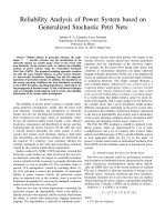
Fig.1 shows a typical GSPN for M/M/1/1/3. In the figure, p
1
, p
2
, p
3
, p
4
,

and p
5
are places; t
1

and t
3
are the timed transitions; t
2
is an immediate transition; and
1

and
3

are the firing

rates for transitions t
1
and t
3
.

Fig. 1. Sample GSPN

2.2 Reachability Graph and Markov Chain
In the example net, the transition t
1
fires after the time determined by the exponential
probability distribution function with parameter
1

, and the tokens in places p
4

and p
5
move
to place p
1
. The assignment of tokens to places is called marking. In this example, the
marking changes from the initial marking m
0
to the next marking m
1
when t
1
fires, as shown
in Fig.2. The change in markings is represented by Equation (2). In Equation (2),
110
[ mtm 
indicates that the marking m
0
changes to m
1
after the transition t
1
fires.
033122110
0322110
[[[[
[[[
mtmtmtmtm
mtmtmtm



(2)
00131
00120
11010
01021
m
0
m
1
m
2
m
3
t
1
t
2
t
1
t
3
t
3
(p
1
,p
2
,p
3

,p
4
,p
5
)
00131
00120
11010
01021
m
0
m
1
m
2
m
3
t
1
t
2
t
1
t
3
t
3
(p
1
,p

2
,p
3
,p
4
,p
5
)

Fig. 2. Reachability graph for the sample GSPN.

The set of markings reached from m
0
is called a reachability set and is defined as follows:
[Definition 2]
The minimum set of markings satisfying the following condition is called the reachability
set of the initial marking m
0
and is represented by RS(m
0
).
AnApplicationofGSPNforModelingandEvaluatingLocalAreaComputerNetworks 3

(Imai et al., 1997;Kumagai et al., 2003). GSPNs are an extension of the Petri Nets that can be
easily used to model the timing behavior of systems. The tagged task approach can reduce the
number of states in a model by tracing the behavior of a tagged task.
A method for evaluating local area computer network systems, such as the IEEE802.11e
WLAN supporting EDCA, based on delay jitter analysis using the Generalized Stochastic
Petri Net (GSPN) and the tagged task approach, is fully explained. The system is modeled
using GSPN with the tagged task approach, then the state transition diagram of the Markov

chain is constructed from the reduced reachability graph of the GSPN model. Processing
paths are extracted, and the mean value and variance of the delay time are calculated using
the equations derived from the Markov chain. An evaluation example is also given. Section
2 explains system modelling using GSPN, while Section 3 presents the evaluation method
that will be used. Section 4 describes the evaluation example, which is a system built using
IEEE802.11e WLAN supporting EDCA. Finally, Section 5 summarizes the results of this
chapter.

2. Modeling Network Systems Using GSPN
2.1 GSPN
GSPN can be defined as follows (Marson et al., 1995). The set of all natural numbers will be
denoted as N, while the set of all real numbers will be denoted as R.
[Definition1]
),,,,,,,(
0
MWWWTPN
h
GSPN



(1)
 
nPipP
i
 1
; Set of places,


mTjtT

j
 1
; Set of transitions,




TITI
TTTTT ,
;
I
T
is a set of immediate transitions,
T
T
is a set of timed
transitions,
NTPW 

: ; Input connection function,
NPTW 

: ; Output connection function,
NTPW
h
:
; Inhibitor arcs,


Ti

Ti  1

; Firing rates,
RT
I
:

; Weighting function of immediate transitions,
0
m : Initial marking.
In GSPN, places are represented by circles; timed transitions by boxes; and immediate
transitions by thin bars. An inhibitor arc ends in a small circle. A timed transition fires
according to the firing rate assigned to the transition when the firing condition is satisfied.
Fig.1 shows a typical GSPN for M/M/1/1/3. In the figure, p
1
, p
2
, p
3
, p
4
,

and p
5
are places; t
1

and t
3

are the timed transitions; t
2
is an immediate transition; and
1

and
3

are the firing
rates for transitions t
1
and t
3
.

Fig. 1. Sample GSPN

2.2 Reachability Graph and Markov Chain
In the example net, the transition t
1
fires after the time determined by the exponential
probability distribution function with parameter
1

, and the tokens in places p
4
and p
5
move
to place p
1
. The assignment of tokens to places is called marking. In this example, the
marking changes from the initial marking m
0
to the next marking m
1
when t
1
fires, as shown
in Fig.2. The change in markings is represented by Equation (2). In Equation (2),
110
[ mtm 
indicates that the marking m
0
changes to m
1
after the transition t

1
fires.
033122110
0322110
[[[[
[[[
mtmtmtmtm
mtmtmtm


(2)
00131
00120
11010
01021
m
0
m
1
m
2
m
3
t
1
t
2
t
1
t

3
t
3
(p
1
,p
2
,p
3
,p
4
,p
5
)
00131
00120
11010
01021
m
0
m
1
m
2
m
3
t
1
t
2

t
1
t
3
t
3
(p
1
,p
2
,p
3
,p
4
,p
5
)

Fig. 2. Reachability graph for the sample GSPN.

The set of markings reached from m
0
is called a reachability set and is defined as follows:
[Definition 2]
The minimum set of markings satisfying the following condition is called the reachability
set of the initial marking m
0
and is represented by RS(m
0
).

PetriNets:Applications4

)(
[:)(
),(
02
2101
00
mRSm
mtmTtmRSm
mRSm



(3)
The change of markings in a reachability set can be represented by a graph. The graph of all
reachable markings from the initial marking is called the reachability graph and is defined
as follows.
[Definition 3]
A labeled digraph is called a reachability graph and is represented by RG(m
0
) when the set
of nodes in the graph is RS(m
0
), and the set of edges A in the graph is defined by the
following equation:
)(,,[),,(
)()(
0
00

mRSmmmtmAtmm
TmRSmRSA
jijiji


(4)

The GSPN has two kinds of markings: tangible and vanishing. Tangible markings allow
timed transitions to fire, while vanishing markings allow immediate transitions to fire.
Vanishing markings can be reduced by eliminating them from the reachability graph. The
reduced reachability graph is equivalent to the state transition diagram of a Markov chain
for the GSPN model (Marson et al., 1995) and is shown in Fig.3.

Fig. 3. State diagram of the Markov chain for the sample GSPN.

3. System Model
In network systems processing multimedia data with QoS control, tasks are processed
according to their priorities for satisfying their QoS requirement. The following system
assumptions are useful for analysis.
[Assumption1]
Each task has a priority, which determines when it is processed and delivered.
m
0
m
2
m
3
1

1


3

3

m
0
m
2
m
3
1

1

3

3


In network systems containing many hosts, tasks occur randomly, and the processing time
for tasks may be an arbitrary value. Thus, the following assumptions are made about the
tasks:
[Assumption2]
(1) Tasks occur according to a Poisson process.
(2) Task processing time is determined by the exponential probability distribution function.
The IEEE 802.11e WLAN supporting EDCA is used as the example for explaining the system
model and the evaluation method. The IEEE 802.11e WLAN supporting EDCA has four
access categories (ACs): AC_VO, AC_VI, AC_BE, and AC_BK. The access category AC_VO
is the category for voice tasks and has the highest priority. AC_VI is the category for video

and has the second-highest priority. AC_BE is the category for best-effort tasks and has the
third-highest priority. AC_BK is the category for background tasks and has the lowest
priority. The GSPN model for analyzing mean delay and its jitter for the AC_VO task is
shown in Fig.4 (Ikeda et al., 2005) (Tsunoyama et al., 2008). The model is constructed based
on the tagged task approach in order to decrease the increase in the number of states in the
Markov chain.

(a) Target host part.

AnApplicationofGSPNforModelingandEvaluatingLocalAreaComputerNetworks 5

)(
[:)(
),(
02
2101
00
mRSm
mtmTtmRSm
mRSm



(3)
The change of markings in a reachability set can be represented by a graph. The graph of all
reachable markings from the initial marking is called the reachability graph and is defined
as follows.
[Definition 3]
A labeled digraph is called a reachability graph and is represented by RG(m
0
) when the set
of nodes in the graph is RS(m
0
), and the set of edges A in the graph is defined by the
following equation:
)(,,[),,(

)()(
0
00
mRSmmmtmAtmm
TmRSmRSA
jijiji


(4)

The GSPN has two kinds of markings: tangible and vanishing. Tangible markings allow
timed transitions to fire, while vanishing markings allow immediate transitions to fire.
Vanishing markings can be reduced by eliminating them from the reachability graph. The
reduced reachability graph is equivalent to the state transition diagram of a Markov chain
for the GSPN model (Marson et al., 1995) and is shown in Fig.3.

Fig. 3. State diagram of the Markov chain for the sample GSPN.

3. System Model
In network systems processing multimedia data with QoS control, tasks are processed
according to their priorities for satisfying their QoS requirement. The following system
assumptions are useful for analysis.
[Assumption1]
Each task has a priority, which determines when it is processed and delivered.
m
0
m
2
m
3

1

1

3

3

m
0
m
2
m
3
1

1

3

3


In network systems containing many hosts, tasks occur randomly, and the processing time
for tasks may be an arbitrary value. Thus, the following assumptions are made about the
tasks:
[Assumption2]
(1) Tasks occur according to a Poisson process.
(2) Task processing time is determined by the exponential probability distribution function.
The IEEE 802.11e WLAN supporting EDCA is used as the example for explaining the system

model and the evaluation method. The IEEE 802.11e WLAN supporting EDCA has four
access categories (ACs): AC_VO, AC_VI, AC_BE, and AC_BK. The access category AC_VO
is the category for voice tasks and has the highest priority. AC_VI is the category for video
and has the second-highest priority. AC_BE is the category for best-effort tasks and has the
third-highest priority. AC_BK is the category for background tasks and has the lowest
priority. The GSPN model for analyzing mean delay and its jitter for the AC_VO task is
shown in Fig.4 (Ikeda et al., 2005) (Tsunoyama et al., 2008). The model is constructed based
on the tagged task approach in order to decrease the increase in the number of states in the
Markov chain.

(a) Target host part.

PetriNets:Applications6

(b) Nontarget host part.
Fig. 4. GSPN Model of AC_VO in IEEE802.11e WLAN.

In this example, the mean delay and its jitter are analyzed for the AC_VO task generated
from a host. In the analysis, the AC_VO task is called the tagged task, and the host is called
the target host. Fig.4 (a) shows part of the model and represents the behavior of the tasks
from the target host. The right part of the figure represents the interaction between the tasks
of the other access categories in the target host and the tasks from the nontarget hosts in the
WLAN. Fig.4 (b) also shows part of the model and represents the behavior of tasks from the
nontarget hosts in the WLAN.
When an AC_VO task is generated in the target host, the transition T_gen_vo fires, and a
token moves from P_gen_vo to P_back_vo. After the back-off time, T_back_vo fires and the
token moves to P_trans. If no task is being sent from the nontarget hosts, the token moves to
P_trans_succ and also moves back to P_gen_vo, since no collision occurs. If another task is
being sent from the nontarget hosts, the token moves to P_timeout and moves to P_trans_fail
after the time determined by the firing rate for T_timeout. When a task with another access
category is generated from the target host, the transition T_gen_q fires and a token moves to
P_back_q. The collision is examined by T_fail and T_timeout, as with AC_VO.

4. Evaluation Method
4.1 Delivery path and its selection probability
The delay time for task processing can be obtained by accumulating the sojourn time for
states in a state sequence from a start state, where the task occurs, to an end state, where the
task has been processed and delivered successfully. A reduced reachability graph is
equivalent to a state diagram of a Markov chain for task processing. Thus, the delay time
can be obtained from the firing rate of transitions in the path corresponding to the state
sequence. A path in a reduced reachability graph is defined by the following definition. In
the definition,

)( biam
i


are markings and
)(




jt
j
are transitions.
[Definition4]
A sequence of markings and transitions, m
a
[ t
α
> … m
c
>t
β
> m
b
], starting at marking m
a
and
ending at marking m
b
, for a reduced reachability graph is called a path from m

a
to m
b
. The
number of paths from m
a
to m
b
is denoted by N
ab
, while the i
th
path is denoted by P
ab
(i)
(1 ≤ i ≤
N
ab
).
When there are a number of paths from start marking m
a
to end marking m
b
, task processing
is made along one of the paths with the given probability. The probability of a path selected
in all paths from m
a
to m
b
is called the path selection probability and is denoted by P

r
(P
ab
(i)
|
m
a
), where 1 ≤ i ≤ N
ab
.
The probability of transition from marking m
j
to next marking m
k
is determined by the
following equation, where A
j
is the set of subscripts of outgoing arcs from the marking m
j
(Marson et. al., 1995).





j
Al
lj
j
j

kj
mm


,)Pr(
(4)
The path selection probability for path P
ab
(i)
is obtained by the product of the above
probabilities for a path and given by the following lemma (Kumagai et al., 2003).
[Lemma1]




c
aj
j
n
a
i
ab
j
mP

)|Pr(
)(
(5)

4.2 Sojourn Time for the Path and Delay Jitter
The sojourn time for a path is given by the summation of the sojourn time for all markings
in the path. Therefore, the probability density function of the sojourn time for a path can be
obtained by the convolution of the probability density function of the sojourn time for every
marking in the path. The probability density function of sojourn time,
)(i
ab

, for path P
ab
(i)

can be obtained using Equation (5) and Assumption 2. The result is given by the following
lemma (Kumagai et al., 2003).
[Lemma2]

























b
aj
b
am
b
mn
an
nm
m
j
t
tf
i
ab
)(
)exp(
)()(
)(

(6)
AnApplicationofGSPNforModelingandEvaluatingLocalAreaComputerNetworks 7

from the target host. The right part of the figure represents the interaction between the tasks
of the other access categories in the target host and the tasks from the nontarget hosts in the
WLAN. Fig.4 (b) also shows part of the model and represents the behavior of tasks from the
nontarget hosts in the WLAN.
When an AC_VO task is generated in the target host, the transition T_gen_vo fires, and a
token moves from P_gen_vo to P_back_vo. After the back-off time, T_back_vo fires and the
token moves to P_trans. If no task is being sent from the nontarget hosts, the token moves to
P_trans_succ and also moves back to P_gen_vo, since no collision occurs. If another task is
being sent from the nontarget hosts, the token moves to P_timeout and moves to P_trans_fail
after the time determined by the firing rate for T_timeout. When a task with another access
category is generated from the target host, the transition T_gen_q fires and a token moves to
P_back_q. The collision is examined by T_fail and T_timeout, as with AC_VO.

4. Evaluation Method
4.1 Delivery path and its selection probability
The delay time for task processing can be obtained by accumulating the sojourn time for
states in a state sequence from a start state, where the task occurs, to an end state, where the
task has been processed and delivered successfully. A reduced reachability graph is
equivalent to a state diagram of a Markov chain for task processing. Thus, the delay time
can be obtained from the firing rate of transitions in the path corresponding to the state
sequence. A path in a reduced reachability graph is defined by the following definition. In
the definition,
)( biam
i

are markings and
)(





jt
j
are transitions.
[Definition4]
A sequence of markings and transitions, m
a
[ t
α
> … m
c
>t
β
> m
b
], starting at marking m
a
and
ending at marking m
b
, for a reduced reachability graph is called a path from m
a
to m
b
. The
number of paths from m
a
to m
b

is denoted by N
ab
, while the i
th
path is denoted by P
ab
(i)
(1 ≤ i ≤
N
ab
).
When there are a number of paths from start marking m
a
to end marking m
b
, task processing
is made along one of the paths with the given probability. The probability of a path selected
in all paths from m
a
to m
b
is called the path selection probability and is denoted by P
r
(P
ab
(i)
|
m
a
), where 1 ≤ i ≤ N

ab
.
The probability of transition from marking m
j
to next marking m
k
is determined by the
following equation, where A
j
is the set of subscripts of outgoing arcs from the marking m
j
(Marson et. al., 1995).





j
Al
lj
j
j
kj
mm


,)Pr(
(4)
The path selection probability for path P
ab

(i)
is obtained by the product of the above
probabilities for a path and given by the following lemma (Kumagai et al., 2003).
[Lemma1]




c
aj
j
n
a
i
ab
j
mP

)|Pr(
)(
(5)

4.2 Sojourn Time for the Path and Delay Jitter
The sojourn time for a path is given by the summation of the sojourn time for all markings
in the path. Therefore, the probability density function of the sojourn time for a path can be
obtained by the convolution of the probability density function of the sojourn time for every
marking in the path. The probability density function of sojourn time,
)(i
ab


, for path P
ab
(i)

can be obtained using Equation (5) and Assumption 2. The result is given by the following
lemma (Kumagai et al., 2003).
[Lemma2]

























b
aj
b
am
b
mn
an
nm
m
j
t
tf
i
ab
)(
)exp(
)()(
)(

(6)
PetriNets:Applications8

The mean value

E
and the variance

V
of the delay time can be obtained from Equation (6).

The following results are presented as a theorem: (Ikeda et al., 2005;Kumagai et al., 2003).
[Theorem1]
 


 




























ab
gen
N
i
b
aj
b
jk
ak
kj
k
j
a
i
ab
Sa
a
mPmE
1
)(
1
)|Pr()Pr(

(7)
 



 







































ab
gen
N
i
b
aj
b
jk
ak
kj
k
j
a
i
ab
Sa
a
EmPmV
1
2
2

)(
2
)|Pr()Pr(

(8)

4.3 Evaluation procedure
Fig.5 shows a flow chart for evaluation. A network is first modeled using GSPN. The GSPN
model is then analyzed and a reachability graph is obtained using the Petri Net tool, Time
Net (German et al., 1995). The set of start markings is extracted from the reachability graph,
and the delivery paths are searched. The delay time and its jitter are calculated for all
searched delivery paths.

Fig. 5. Flow chart of the method.

5. Example
An example network using IEEE802.11e over the IEEE802.11a consisting of three hosts is
evaluated. Table 1 shows the parameters for the simulation.

Start
Modellin
g
WLAN usin
g
GSPN

Analyse the model using Time Net.

Extract Sgen and search the delivery paths.
Calculate mean and standard deviation of the
delay time.
End

Access
Categories

AIFSN CW min CW max TXOP
Limit
AC_BK 7 15 1023 1 frame

AC_BE 3 15 1023 1 frame
AC_VI 2 7 15 3 ms
AC_VO 2 3 7 1.5 ms
Table 1. Parameters for the ACs.

Each AC has four parameters, and ACs are distinguished by assigning different values to
the parameters. Table 1 shows the default values for the parameters. A smaller value implies
a higher priority. In the example, AC_VO is first analyzed by assigning a tagged task, and
then AC_VI is analyzed.
Figs.3 and 4 show the mean delay and jitter for AC_VO and AC_VI, respectively. The
figures show that the mean delay for AC_VI increases by about 7.5 [ms] and the jitter for
AC_VI increases by about 4.3 [ms] when the virtual load on the network increases from 0.1
to 10.0 . However, when the virtual load increases, the mean delay and jitter for AC_VO
decrease by about 1 [ms] less than AC_VI (Ikeda et al., 2005) (Tsunoyama & Imai 2008).

Fig. 6. Mean delay time for AC_VO and AC_VI.

AnApplicationofGSPNforModelingandEvaluatingLocalAreaComputerNetworks 9

The mean value

E
and the variance

V
of the delay time can be obtained from Equation (6).
The following results are presented as a theorem: (Ikeda et al., 2005;Kumagai et al., 2003).
[Theorem1]
 



 



























ab

gen
N
i
b
aj
b
jk
ak
kj
k
j
a
i
ab
Sa
a
mPmE
1
)(
1
)|Pr()Pr(

(7)
 


 








































ab
gen
N
i
b
aj
b
jk
ak
kj
k
j
a
i
ab
Sa
a
EmPmV
1
2
2
)(
2
)|Pr()Pr(


(8)

4.3 Evaluation procedure
Fig.5 shows a flow chart for evaluation. A network is first modeled using GSPN. The GSPN
model is then analyzed and a reachability graph is obtained using the Petri Net tool, Time
Net (German et al., 1995). The set of start markings is extracted from the reachability graph,
and the delivery paths are searched. The delay time and its jitter are calculated for all
searched delivery paths.

Fig. 5. Flow chart of the method.

5. Example
An example network using IEEE802.11e over the IEEE802.11a consisting of three hosts is
evaluated. Table 1 shows the parameters for the simulation.

Start
Modellin
g
WLAN usin
g
GSPN

Analyse the model using Time Net.

Extract Sgen and search the delivery paths.
Calculate mean and standard deviation of the
delay time.
End

Access
Categories
AIFSN CW min CW max TXOP
Limit
AC_BK 7 15 1023 1 frame
AC_BE 3 15 1023 1 frame
AC_VI 2 7 15 3 ms
AC_VO 2 3 7 1.5 ms
Table 1. Parameters for the ACs.

Each AC has four parameters, and ACs are distinguished by assigning different values to
the parameters. Table 1 shows the default values for the parameters. A smaller value implies
a higher priority. In the example, AC_VO is first analyzed by assigning a tagged task, and
then AC_VI is analyzed.
Figs.3 and 4 show the mean delay and jitter for AC_VO and AC_VI, respectively. The
figures show that the mean delay for AC_VI increases by about 7.5 [ms] and the jitter for
AC_VI increases by about 4.3 [ms] when the virtual load on the network increases from 0.1
to 10.0 . However, when the virtual load increases, the mean delay and jitter for AC_VO
decrease by about 1 [ms] less than AC_VI (Ikeda et al., 2005) (Tsunoyama & Imai 2008).

Fig. 6. Mean delay time for AC_VO and AC_VI.

PetriNets:Applications10

Fig. 7. Jitter for AC_VO and AC_VI.

6. Conclusions
A method for modelling local area computer networks used for processing and delivering
multimedia data is proposed. The proposed method can evaluate the mean delay time and
its jitter (standard deviation) for systems based on the GSPN model and tagged task
approach. The systems can be modeled by the method presented, and both of the values can
be evaluated easily using the equations shown in this chapter. An example of modeling and
evaluating local area computer networks using IEEE802.11e WLAN supporting EDCA was
shown. From the results, it can be concluded that the system can be modeled easily. The
mean delay and jitter for AC_VO obtained using the proposed method agrees well with the
values obtained using simulations. However, when the virtual load of the network exceeds
one, the value of the jitter for AC_VI differs slightly from that by simulation.
Future efforts will improve the model to reduce the observed difference and to compose a
compact model to reduce the number of states in the Markov chain for the network.

7. Acknowledgements
The authors would like to thank Messrs. Kumagai, Ikeda, and Maruyama for their helpful
discussions and comments. The authors would also like to thank Professor Ishii and
Professor Makino for their helpful comments.

8. References
Adachi, N.; Kasahara, S. ; Asahara Y. & Takahashi, Y. (1998). Simulation Study on Multi-
Hop Jitter Behavior in Integrated ATM Network with CATV and Internet, The
Transactions of the Institute of Electronics, Information and Communication Engineers,
Vol. E81-B, No.12, pp.2413-2422.
Ahmad, S. ; Awan, I. & Ahmad, B. (2007). Performance Modeling of Finite Capacity Queues
with Complete Buffer Partitioning Scheme for Bursty Traffic, Proceedings of the
First Asia International Conference on Modeling & Simulation (AMS'07), pp. 264-269.
Althun, B. & Zimmermann, M. (2003). Multimedia Streaming Services: Specification, Imple-
mentation, and Retrieval, Proceedings of the 5th ACM SIGMM International
Workshop on Multimedia Information Retrieval, pp.247-254.
Bin, S.; Latif, A.; Rashid, M.A. & Alam, F. (2007). Profiling Delay and Throughput
Characteristics of Interactive Multimedia Traffic over WLANs Using OPNET,
Proceedings of the 21st International Conference on Advanced Information Networking and
Applications Workshops (AINAW'07) , pp. 929-933.
Cheng, S.T. & Wu, M. (2005). Performance Evaluation of Ad-Hoc WLAN by M/G/1
Queuing Model, Proceedings of the International Conference on Information Technology:
Coding and Computing (ITCC'05), Vol. II, pp. 681-686.
Claypool，M. & Tanner, J. (1999)．The Effect of Jitter on the Perceptual Quality of Video,
ACM Multimedia ’99, pp.115-118.
Fan, Y.; Huang, C.Y. & Tseng, Y.L. (2006). Multimedia Services in IEEE 802.11e WLAN
Systems, Proceedings of the 2006 International Conference on Wireless
communications and mobile computing, pp.401 – 406.

Ferguson, P. & Huston, G. (1998). Quality of Service: Delivering QoS on the Internet and in
Corporate Networks, John Wiley & Sons, Inc.
German, R. (2000). Performance Analysis of Communication Systems with Non-Markovian
Stochastic Petri Nets, John Wiley & Sons, Inc.
German, R.; Kelling, C.; Zimmermann, A. & Hommel, G. (1995). TimeNET-a toolkit for
evaluating non-Markovian stochastic Petrinets, Proceedings of the Sixth International
Workshop on Petri Nets and Performance Models, pp.210-211.
Gibson, L. & David, R. (2007). Streaming Multimedia Delivery in Web Services Based e-
Learning Platforms, Proceedings of the IEEE International Conference on Advanced
Learning Technologies, pp. 706-710.
Grinnemo, K.J. & Brunstrom, A. (2002). A Simulation Based Performance Analysis of a TCP
Extension for Best-Effort Multimedia Applications, Proceedings of the 35th Annual
Simulation Symposium, pp.327.
IEEE Standards Board (2003). Wireless LAN Medium Access Control (MAC) and Physical
Layer (PHY) Specification: Medium Access Control (MAC) Enhancements for
Quality of Service (QoS), IEEE Draft 802.11e, Rev. D5.1.
Ikeda, N.; Imai, H.; Tsunoyama, M. & Ishii, I. (2005). An Evaluation of Mean Delay and Jitter
for 802.11e WLAN, Proceedings of the Fourth IASTED International Conference on
Communication Systems and Networks, pp.202-206, Sept.
Imai, H.; Tsunoyama, M.; Ishii, I.; & Makino, H. (1997). An Analyzing Method for Tagged-T
ask-Model, The Transactions of the Institute of Electronics, Information and
Communication Engineers D-I, Vol.J80-D-1, No.10, pp.836-844.
AnApplicationofGSPNforModelingandEvaluatingLocalAreaComputerNetworks 11

Fig. 7. Jitter for AC_VO and AC_VI.

6. Conclusions
A method for modelling local area computer networks used for processing and delivering
multimedia data is proposed. The proposed method can evaluate the mean delay time and

its jitter (standard deviation) for systems based on the GSPN model and tagged task
approach. The systems can be modeled by the method presented, and both of the values can
be evaluated easily using the equations shown in this chapter. An example of modeling and
evaluating local area computer networks using IEEE802.11e WLAN supporting EDCA was
shown. From the results, it can be concluded that the system can be modeled easily. The
mean delay and jitter for AC_VO obtained using the proposed method agrees well with the
values obtained using simulations. However, when the virtual load of the network exceeds
one, the value of the jitter for AC_VI differs slightly from that by simulation.
Future efforts will improve the model to reduce the observed difference and to compose a
compact model to reduce the number of states in the Markov chain for the network.

7. Acknowledgements
The authors would like to thank Messrs. Kumagai, Ikeda, and Maruyama for their helpful
discussions and comments. The authors would also like to thank Professor Ishii and
Professor Makino for their helpful comments.

8. References
Adachi, N.; Kasahara, S. ; Asahara Y. & Takahashi, Y. (1998). Simulation Study on Multi-
Hop Jitter Behavior in Integrated ATM Network with CATV and Internet, The
Transactions of the Institute of Electronics, Information and Communication Engineers,
Vol. E81-B, No.12, pp.2413-2422.
Ahmad, S. ; Awan, I. & Ahmad, B. (2007). Performance Modeling of Finite Capacity Queues
with Complete Buffer Partitioning Scheme for Bursty Traffic, Proceedings of the
First Asia International Conference on Modeling & Simulation (AMS'07), pp. 264-269.
Althun, B. & Zimmermann, M. (2003). Multimedia Streaming Services: Specification, Imple-
mentation, and Retrieval, Proceedings of the 5th ACM SIGMM International
Workshop on Multimedia Information Retrieval, pp.247-254.
Bin, S.; Latif, A.; Rashid, M.A. & Alam, F. (2007). Profiling Delay and Throughput
Characteristics of Interactive Multimedia Traffic over WLANs Using OPNET,

Proceedings of the 21st International Conference on Advanced Information Networking and
Applications Workshops (AINAW'07) , pp. 929-933.
Cheng, S.T. & Wu, M. (2005). Performance Evaluation of Ad-Hoc WLAN by M/G/1
Queuing Model, Proceedings of the International Conference on Information Technology:
Coding and Computing (ITCC'05), Vol. II, pp. 681-686.
Claypool，M. & Tanner, J. (1999)．The Effect of Jitter on the Perceptual Quality of Video,
ACM Multimedia ’99, pp.115-118.
Fan, Y.; Huang, C.Y. & Tseng, Y.L. (2006). Multimedia Services in IEEE 802.11e WLAN
Systems, Proceedings of the 2006 International Conference on Wireless
communications and mobile computing, pp.401 – 406.
Ferguson, P. & Huston, G. (1998). Quality of Service: Delivering QoS on the Internet and in
Corporate Networks, John Wiley & Sons, Inc.
German, R. (2000). Performance Analysis of Communication Systems with Non-Markovian
Stochastic Petri Nets, John Wiley & Sons, Inc.
German, R.; Kelling, C.; Zimmermann, A. & Hommel, G. (1995). TimeNET-a toolkit for
evaluating non-Markovian stochastic Petrinets, Proceedings of the Sixth International
Workshop on Petri Nets and Performance Models, pp.210-211.
Gibson, L. & David, R. (2007). Streaming Multimedia Delivery in Web Services Based e-
Learning Platforms, Proceedings of the IEEE International Conference on Advanced
Learning Technologies, pp. 706-710.
Grinnemo, K.J. & Brunstrom, A. (2002). A Simulation Based Performance Analysis of a TCP
Extension for Best-Effort Multimedia Applications, Proceedings of the 35th Annual
Simulation Symposium, pp.327.
IEEE Standards Board (2003). Wireless LAN Medium Access Control (MAC) and Physical
Layer (PHY) Specification: Medium Access Control (MAC) Enhancements for
Quality of Service (QoS), IEEE Draft 802.11e, Rev. D5.1.
Ikeda, N.; Imai, H.; Tsunoyama, M. & Ishii, I. (2005). An Evaluation of Mean Delay and Jitter
for 802.11e WLAN, Proceedings of the Fourth IASTED International Conference on
Communication Systems and Networks, pp.202-206, Sept.
Imai, H.; Tsunoyama, M.; Ishii, I.; & Makino, H. (1997). An Analyzing Method for Tagged-T

ask-Model, The Transactions of the Institute of Electronics, Information and
Communication Engineers D-I, Vol.J80-D-1, No.10, pp.836-844.
PetriNets:Applications12

Imai, H.; Tsunoyama. M.; Ishii, I. & Makino, H. (1999). Modeling and Evaluating Computer
Systems for Multimedia Data Processing, Proceedings of the Eighteenth IASTED
International Conference on Modeling, Identification and Control, pp.353-358.
Kornkevn, S. & Lilleberg, N. (2002). Enhancing support and learning services for instructors
and students who engage in course-related multimedia and web projects,
Proceedings of the 30th annual ACM SIGUCCS Conference on User services, pp.56-59.
Kumagai, K.; Tsunoyama, M.; Imai, H., & Ishii, I. (2003). An evaluation Method for
Network Systems based on Delay Jitter Analysis”, Proceedings of the 4-th
EURASIP Conference focused on Video/Image Processing and Multimedia
Communications, pp.569-574.
Marson, M.A.; Balvo, G.; Conte, G.; Donatelli, S.
& Franceschinis, G. (1995). Modeling with
Generalized Stochastic Petri Nets, John Wiley & Sons, Inc.
Nerjes, G.; Muth, P. & Weikum, G. (1997).Stochastic Performance Guarantees for Mixed
Workloads in a Multimedia Information System, Proceedings of the 7th International
Workshop on Research Issues in Data Engineering (RIDE '97), pp. 131.
Park, S. (2006). DiffServ Quality of Service Support for Multimedia Applications in
Broadband Access Networks, Proceedings of the 2006 International Conference on
Hybrid Information Technology, Vol.2, pp. 513-518.
Shahraray, B.; Ma, W.Y.; Zakhor, A., & Babaguchi, N. (2005). Mobile Multimedia Services,
International World Wide Web Conference, pp.795-795.
Tsunoyama, M. & Imai, H. (2008). An Evaluation Method for Delay Time and Its Jitter of
WLAN using GSPN Model, Proceedings of the 8th International Workshop on Wireless
Local Networks (WLN2008), pp.811-812.
Villalon, J.; Mico, F.; Cuenca, P. & Barbosa, L.O. (2005). QoS Support for Time-Constrained
Multimedia Communications in IEEE 802.11 WLANs, Proceedings of the A Perfor-

mance Evaluation, Systems Communications (ICW'05, ICHSN'05, ICMCS'05,
SENET'05), pp. 135-140.
ArchitectureofComputerIntrusionDetectionBasedonPartiallyOrderedEvents 13
ArchitectureofComputerIntrusionDetectionBasedonPartiallyOrdered
Events
LiberiosVokorokosandAntonBaláž
0
Architecture of Computer Intrusion Detection
Based on Partially Ordered Events
Liberios Vokorokos and Anton Baláž
Technical University of Košice
Slovak Republic
1. Introduction
Information technologies became part of our daily life. Nowadays, contemporary society is
dependent on functioning of miscellaneous information systems providing daily community
motion. The attack aim is often to disrupt, deny of service or at least one of its parts required
for proper functionality, or to acquire unauthorized access to information [Vokorokos (2004)].
Nowadays, solid system assecuration becomes one of the main priorities. Basic way
of protection is realized through specialized devices ﬁrewalls allowing to deﬁne and
control permitted communications in boundary parts of computer network or between
protected segments and surrounding environment. Present ﬁrewalls often detect some
unauthorized attack activities but their functionality is limited. Unauthorized intrusion
detection systems allow increase of information systems security against attacks from the
Internet or organization intranet, by means of passive inform about arising intrusion or active
interfere against defecting intrusion.
The existing intrusion detection approaches can be divided in two classes - anomaly detection
and misuse detection [Denning (1987)]. The anomaly detection approaches the problem by
attempting to ﬁnd deviations from the established patterns of usage. On the other hand,
the misuse detection compares the usage patterns to known techniques of compromising
computer security. Architecturally, the intrusion detection system(IDS) can be categorized

into three types - host-based IDS, network-based IDS and hybrid IDS [Bace (2000)]. The
host-based IDS, deployed in individual host-machines, can monitor audit data of a single
host. The network-based IDS monitors the trafﬁc data sent and received by hosts. The hybrid
IDS uses both methods. The intrusion detection through multiple sources represents a difﬁcult
task. Intrusion pattern matching has a non-deterministic nature where that same intrusion or
attack can be realized through various permutations of the same events. The purpose of this
paper is to present authors’ proposed intrusion detection architecture based on the partially
ordered events and the Petri nets.
Project is proposed and implemented at the Department of Computers and Informatics in
Košice supported by VEGA 1/4071/07. (Security architecture of heterogeneous distributed
and parallel computing system and dynamical computing system resistant against attacks)
a APVV 0073-07 (Identiﬁcation methods and analysis of safety threats in architecture of
distributed computer systems and dynamical networks).
2
PetriNets:Applications14
2. State of art
Several intrusion detection systems were designed and implemented till today. Most of these
systems are based on statistical methods derived from work of Denning [Denning (1987)].
Some of them, as source of information, use log system of operation system [Anderson et al.
(1995)]. Other one, as input data, use network trafﬁc [Zhang et al. (2003)] [Spirakis et al. (1994)]
[Servilla (1990)]. Systems, as MADIDS [Guangchun et al. (2003)], extend this network trafﬁc
with distribution of intrusion data within single analyzing network systems that perform
partial intrusion detection. Among systems not working with statistical methods, there can
be inserted system of authors [Teng et al. (1990)] that analyzes single user events and tries to
ﬁnd mutual relations among them. IDS architectures based on misuse detection are systems,
as [Ilgun et al. (1995)] [Ilgun (1993)], that search for already known intrusions, derived state
of intrusion based on present system state.
According to present state of intrusion detection systems, this work is focused on intrusion
detection and system penetration variability, which can reduce time needed to evaluate
potential intrusion.

3. Architecture of designed IDS system
Proposed system architecture includes part of planning and matching, ﬁgure 1. The matching
means that the system gets into a state of intrusion when a sequence of events leading to
the mentioned state occurs. The intrusion is a system state which overtakes previous states
represented by particular system events. If there exists such a ﬁne-grained log system, it is
possible to detect the states with intrusion. Single attacks to the systems represents mentioned
single events that in a ﬁnal implication leads to the state of intrusion. Characteristic feature
of intrusions is their variability; permutation of same events leads to same state of intrusion.
Single intrusions are characteristic with their non-determination. Designed IDS system solves
this problem with planning [Russell & Norvig (2003)] that responds to lay-out of possible
sequence of steps leading to the ﬁnal intrusion. Planning part creates the intrusion plan by
ﬁrst-order logic when it describes known activities and disturber’s goals to specify attack
sequences. Result of planning is intrusion speciﬁcation and its single steps that uses the
matching part of the system to the intrusion detection provided by Petri Net automata. System
architecture designed on the Department of Computers and Informatics is on the ﬁgure 1.
4. Partially ordered state analysis
One of the main problems related to the intrusion detection of the system refers to the
variability of possible attacks. It is possible to realize the same attack by many ways.
Suggested IDS architecture uses the analysis of partially ordered states in a difference from
the classical analysis of the transition by the states of the monitored system. In the classical
scheme of the state analysis [Axelsson (2000)], the attacks are represented as a sequence of
the transition states. States in the scheme of the attack correspond with the states of the
system that have their Boolean statement related to these states. These expressions must
fulﬁll the conditions to realize the transition to the next state. The constituent next states are
interconnected by the oriented paths that represent events or conditions for the change of the
states. Such a state diagram represents the actual state of the monitored system. The change of
the states considers about the intrusion as the event sequence that is realized by the attacker.
These events start in the initial state and end in the ﬁnal compromised state. The initial state
represents the states of the system before starting the penetration. The ﬁnal compromised state
Client

Knowle dge basis
XML Intrusion des cription
Eventsplanning
Java Class
Java Byte Code
Server
Events e valuation
Petri Net
1

Events e valuation
Petri Net
n
Output
Audit
TCPDump
C2 log
TCP/IP-protocol
Fig. 1. Architecture of Designed IDS System
represents the state of the system which follows from the ﬁnished penetration. The transition
of the states that the intruder must do for the achievement of the ﬁnal result of the system
intrusion, are among the initial and ﬁnal states. In the ﬁgure 2 there is an example of the
attack that consists of four states of the attack.
Classical method of the state transition [Anderson (1980)] strictly analyzes intrusion
signatures as ordered sequence of states without any chance of overlaying sequence of single
ArchitectureofComputerIntrusionDetectionBasedonPartiallyOrderedEvents 15
2. State of art
Several intrusion detection systems were designed and implemented till today. Most of these

systems are based on statistical methods derived from work of Denning [Denning (1987)].
Some of them, as source of information, use log system of operation system [Anderson et al.
(1995)]. Other one, as input data, use network trafﬁc [Zhang et al. (2003)] [Spirakis et al. (1994)]
[Servilla (1990)]. Systems, as MADIDS [Guangchun et al. (2003)], extend this network trafﬁc
with distribution of intrusion data within single analyzing network systems that perform
partial intrusion detection. Among systems not working with statistical methods, there can
be inserted system of authors [Teng et al. (1990)] that analyzes single user events and tries to
ﬁnd mutual relations among them. IDS architectures based on misuse detection are systems,
as [Ilgun et al. (1995)] [Ilgun (1993)], that search for already known intrusions, derived state
of intrusion based on present system state.
According to present state of intrusion detection systems, this work is focused on intrusion
detection and system penetration variability, which can reduce time needed to evaluate
potential intrusion.
3. Architecture of designed IDS system
Proposed system architecture includes part of planning and matching, ﬁgure 1. The matching
means that the system gets into a state of intrusion when a sequence of events leading to
the mentioned state occurs. The intrusion is a system state which overtakes previous states
represented by particular system events. If there exists such a ﬁne-grained log system, it is
possible to detect the states with intrusion. Single attacks to the systems represents mentioned
single events that in a ﬁnal implication leads to the state of intrusion. Characteristic feature
of intrusions is their variability; permutation of same events leads to same state of intrusion.
Single intrusions are characteristic with their non-determination. Designed IDS system solves
this problem with planning [Russell & Norvig (2003)] that responds to lay-out of possible
sequence of steps leading to the ﬁnal intrusion. Planning part creates the intrusion plan by
ﬁrst-order logic when it describes known activities and disturber’s goals to specify attack
sequences. Result of planning is intrusion speciﬁcation and its single steps that uses the
matching part of the system to the intrusion detection provided by Petri Net automata. System
architecture designed on the Department of Computers and Informatics is on the ﬁgure 1.
4. Partially ordered state analysis
One of the main problems related to the intrusion detection of the system refers to the

variability of possible attacks. It is possible to realize the same attack by many ways.
Suggested IDS architecture uses the analysis of partially ordered states in a difference from
the classical analysis of the transition by the states of the monitored system. In the classical
scheme of the state analysis [Axelsson (2000)], the attacks are represented as a sequence of
the transition states. States in the scheme of the attack correspond with the states of the
system that have their Boolean statement related to these states. These expressions must
fulﬁll the conditions to realize the transition to the next state. The constituent next states are
interconnected by the oriented paths that represent events or conditions for the change of the
states. Such a state diagram represents the actual state of the monitored system. The change of
the states considers about the intrusion as the event sequence that is realized by the attacker.
These events start in the initial state and end in the ﬁnal compromised state. The initial state
represents the states of the system before starting the penetration. The ﬁnal compromised state
Client
Knowle dge basis
XML Intrusion des cription
Eventsplanning
Java Class
Java Byte Code
Server
Events e valuation
Petri Net
1

Events e valuation
Petri Net
n
Output
Audit

TCPDump
C2 log
TCP/IP-protocol
Fig. 1. Architecture of Designed IDS System
represents the state of the system which follows from the ﬁnished penetration. The transition
of the states that the intruder must do for the achievement of the ﬁnal result of the system
intrusion, are among the initial and ﬁnal states. In the ﬁgure 2 there is an example of the
attack that consists of four states of the attack.
Classical method of the state transition [Anderson (1980)] strictly analyzes intrusion
signatures as ordered sequence of states without any chance of overlaying sequence of single
PetriNets:Applications16
s
1
s
2
s
3
s
4
create(object) setuid(object) setuid(object)
exists(object)=false
user!=root
owner(object)=user
setup(object)=false
owner(object)=user
setuid(object)=true
owner(object)!=user
setuid(object)=true
Fig. 2. State Transition Diagram
events. Designed IDS architecture increases the ﬂexibility of states analysis by using partially

ordered events. Partially ordered events specify option when the events are ordered one
according to another while the others are without this option of ordering. Analysis of partially
ordered states enables several event sequences to form one state diagram. By using partially
ordering against total ordering it is possible to use only one diagram to representation
permutation of the same attack. In the proposed architecture partially ordered state transitions
are generated by partially ordered planner. Representation by partially ordered plan is more
indicating according to total ordered form of states. It enables planner to put off or to ignore
unnecessary ordering selection. During the state transition analysis, the number of total
ordering increases exponentially with increasing the number of the states. This property of
complexity coupled with total ordering is eliminated in case of partially ordered planning.
Applying partially ordered notiﬁcation and its property of decomposition, it is possible to
deal with complex domains without any exponential complexity. Partially ordered planner
seeks state space of plans in contrast to state space of cases. The planner begins with a
simple, incomplete plan that is extended in sequence by planner till it gets complete plan
of solution of the problem. The operators in this process are operators on the plans: addition
of steps, instructions appointing order of one step before another and other operations. The
result is ﬁnal plan of order of particular states based on the dependence within these states.
The acquired representation allows through the partly ordered plans to operate a broad
range of troubleshooting domains in the planner as well as systems of intrusion detection.
The partly ordered scheme provides more exact representation of intrusion patterns as the
completely ordered representation, because only inevitable dependencies are considered
within particular events. ﬁgure 3 is the only dependency between operations touch and
chmod.
s
1
s
2
s
3
s

5
s
4
cp
chmod mail
touch
exists(/mail/root)=false
user!=root
owner(/mail/root)=user
setup(/mail/root)=false
owner(/mail/root)=user
setuid(/mail/root)=true
owner(/mail/root)!=user
setuid(/mail/root)=true
exists(x)=false
Fig. 3. Partially Ordered Intrusion States
In the ﬁgure 2, it is not clear which dependencies are necessary within single states. Whereas
in the ﬁgure 3, it is clear which events fore come which. Compromised state in the ﬁgure 3 is
possible represented by the ﬁrst-order logic as:
∃ /var/spool/mail/root x
/var/spool/mail/root
∈ x ∧
own er(/var/spool/mail/root) = root ∧
setuid(/va r/spool/mail/root) = enable
⇒ compromised(x) = true
Proposed approach of intrusion analysis outcomes from the demand assumption of
identiﬁcation of minimal set of intrusion signatures and necessary dependencies within these
signatures. Minimal set of signatures assumes the elimination of irrelevant signatures that do
not create the intrusion. A possible example of attack, creating a link to ﬁle of different owner
with different rights with consequential executing link and obtaining rights of original owner:

1. ls
2. ln
3. cp
4. rm
5. execute
The ﬁrst, third and fourth commands do not have an inﬂuence on the attack; tendency is to
mask the attack. By elimination of these commands, it is possible to get minimal set describing
attack together with single dependencies within events. Example in form of the ﬁrst-order
logic:
ArchitectureofComputerIntrusionDetectionBasedonPartiallyOrderedEvents 17
s
1
s
2
s
3
s
4
create(object) setuid(object) setuid(object)
exists(object)=false
user!=root
owner(object)=user
setup(object)=false
owner(object)=user
setuid(object)=true
owner(object)!=user
setuid(object)=true
Fig. 2. State Transition Diagram
events. Designed IDS architecture increases the ﬂexibility of states analysis by using partially
ordered events. Partially ordered events specify option when the events are ordered one

according to another while the others are without this option of ordering. Analysis of partially
ordered states enables several event sequences to form one state diagram. By using partially
ordering against total ordering it is possible to use only one diagram to representation
permutation of the same attack. In the proposed architecture partially ordered state transitions
are generated by partially ordered planner. Representation by partially ordered plan is more
indicating according to total ordered form of states. It enables planner to put off or to ignore
unnecessary ordering selection. During the state transition analysis, the number of total
ordering increases exponentially with increasing the number of the states. This property of
complexity coupled with total ordering is eliminated in case of partially ordered planning.
Applying partially ordered notiﬁcation and its property of decomposition, it is possible to
deal with complex domains without any exponential complexity. Partially ordered planner
seeks state space of plans in contrast to state space of cases. The planner begins with a
simple, incomplete plan that is extended in sequence by planner till it gets complete plan
of solution of the problem. The operators in this process are operators on the plans: addition
of steps, instructions appointing order of one step before another and other operations. The
result is ﬁnal plan of order of particular states based on the dependence within these states.
The acquired representation allows through the partly ordered plans to operate a broad
range of troubleshooting domains in the planner as well as systems of intrusion detection.
The partly ordered scheme provides more exact representation of intrusion patterns as the
completely ordered representation, because only inevitable dependencies are considered
within particular events. ﬁgure 3 is the only dependency between operations touch and
chmod.
s
1
s
2
s
3
s
5

s
4
cp
chmod mail
touch
exists(/mail/root)=false
user!=root
owner(/mail/root)=user
setup(/mail/root)=false
owner(/mail/root)=user
setuid(/mail/root)=true
owner(/mail/root)!=user
setuid(/mail/root)=true
exists(x)=false
Fig. 3. Partially Ordered Intrusion States
In the ﬁgure 2, it is not clear which dependencies are necessary within single states. Whereas
in the ﬁgure 3, it is clear which events fore come which. Compromised state in the ﬁgure 3 is
possible represented by the ﬁrst-order logic as:
∃ /var/spool/mail/root x
/var/spool/mail/root
∈ x ∧
own er(/var/spool/mail/root) = root ∧
setuid(/va r/spool/mail/root) = enable
⇒ compromised(x) = true
Proposed approach of intrusion analysis outcomes from the demand assumption of
identiﬁcation of minimal set of intrusion signatures and necessary dependencies within these
signatures. Minimal set of signatures assumes the elimination of irrelevant signatures that do
not create the intrusion. A possible example of attack, creating a link to ﬁle of different owner
with different rights with consequential executing link and obtaining rights of original owner:
1. ls

2. ln
3. cp
4. rm
5. execute
The ﬁrst, third and fourth commands do not have an inﬂuence on the attack; tendency is to
mask the attack. By elimination of these commands, it is possible to get minimal set describing
attack together with single dependencies within events. Example in form of the ﬁrst-order
logic:
PetriNets:Applications18
∃ f ile1, f ile2, x
own er
( f ile1) = x ∧
own er( file2) = x ∧
ln( file2, file1) ∧
execute( f ile2) ∧
ln( file2, file1) ≺ execute( f ile2) ∧
⇒
compromised(x)
5. Intrusion signature sequence planning
Intrusion is deﬁned as a set of events with a focus on compromise integrity, conﬁdentiality and
resources availability. Designed architecture of IDS includes the planning part to construct
event sequence plan of which consists the intrusion. Planning includes goals, states and
events. According to what is necessary to do in ﬁnal plans, planning combines actual
environment state with information depending on the ﬁnal result of events.
State transition is characterized as a sequence of events performed by intruders leading from
initial state do ﬁnal compromised state. Planning can be formulated as a problem of state
transition:
• Initial state: Actual state description.
• Final state: Logical expression of concrete system state.
• Intrusion signatures: Events causing change of a system state.

Planning is deﬁned as:
1. Set of single steps of the plan. Every step represents control activity of the plan.
2. Set of ordered dependencies. Every dependency is in a form of S
i
< S
j
, where, step S
i
is executed before S
j
.
3. Set of variable bindings. Every binding is in a v
= x form, where v is a variable in some
step and x is a constant or other variable.
4. Set of causal bindings. Causal binding is in a form of S
i
c
→ S
j
. From state S
i
by auxiliary
c state S
j
, where c is a necessary pre-condition for the S
j
.
Each signature has an associated pre-condition that indicates what has to be completed before
it is possible to apply event bind with the signature. Post-condition expresses event result
connected to the intrusion signature. A task of the planning is to ﬁnd events sequence

responsible for the intrusion. The goal of planning in the designed IDS architecture is to ﬁnd
event sequence and their dependencies and construct result sequence of an intrusion. Partially
ordered planning allows representing plans in which some steps are ordered according to
other steps. Intrusion signatures and their nature of non-determination are suitable for
fundamentals of partially ordered planning. Planning consists of database of intrusions
and events planner - ﬁgure 1. Knowledge base includes information about each intrusion
signature including pre and post conditions of these events in the form of ﬁrst-order logic. The
planner generates set of events and their dependencies for each initial and ﬁnal intrusion state.
Furthermore, knowledge base includes state dependencies for each event signature. This
information is used by planner for deﬁning partially ordering in between intrusion signature.
For instance pre-condition intrusion signature consists of k terms. These are represented in
form of symbols
{PS
1
, PS2, . . . , PS
k
} ∧ {PS
j
< PS
k
} ∧ . . . ∧ {PS
l
< PS
m
}
An algorithm of partially ordered planning begins with minimal plan and in each step this
plan is extended through available pre-condition step. This is realized by selecting intrusion
signature that fulﬁll some of the unfulﬁlled pre-conditions in the plan. For a newly fulﬁlled
pre-conditions of event signatures are causal bindings stored in between them. These bindings
are necessary for partially event ordering. An ordering result is represented by set of events

and their dependencies in between these event signatures. Let intrusion sequence to consist
of n event signatures: SA
1
, SA
2
, . . . , SA
n
, then intrusion structure is speciﬁed as
{SA
1
, SA
2
, . . . , SA
k
} ∧ {SA
j
< SA
k
} ∧ . . . ∧ {SA
l
< SA
m
}
First part of this term {SA
1
, SA
2
, . . . , SA
k
} is a set of event signatures. Next part of the term

is ordering dependency between signatures. The intrusion example referring to ﬁgure 3 is
speciﬁed as
{cp, chmod, touch, mail} ∧ {cp < chmod} ∧ {chmod < mail} ∧ {touch < mail}
Each formulation represents an intrusion signature variation that leads to the same
compromised states. In the case of the intrusion signatures it is necessary to deliberate
this intrusion variability from the view of memory requirements. Further, if it comes to the
alternation of initial state, it may have a consequence of complete intrusion plan alternation.
The next advantage of partially ordered planning is that the time between two intrusion
signatures does not have an inﬂuence on the analysis during capturing system data and state
changing.
5.1 Events planning
This session represents planning algorithm in the designed IDS that’s result is partially
ordered events of intrusion signature. It is possible to represent the intrusive plan through the
triple

A, O, L

, where A is a set of events, O is a set of ordered dependencies on the A set, and
L is a set of casual connections. The planner starts its activity with a blank plan, and it speciﬁes
this plan in stages with being obligated to consideration of consistence requirements deﬁned
in the O set. The key step of this activity is to preserve states of the past conclusions and
requirements for these conclusions. For the provision of consistence within various events,
the recording of relations within the events is performed through the casual connections.
Casual connection is a structure consisting of two references to plan events (producer A
p
and consumer A
c
), and Q assertion that is the result of the A
p
and the A

c
precondition. The
expression is represented by A
p
Q
→ A
c
and connections themselves are stored in the L set.
Casual connections are used for the detection of interference within new and old conclusions.
Marked as threats. This means that

A, O, L

represents a plan and A
p
Q
→ A
c
is a connection
in L. Let the A
t
be another event in A, than the A
t
endangers the A
p
Q
→ A
c
if:
• O

∪ {A
p
< A
t
< A
p
} a
• A
t
has ¬Q as the result
ArchitectureofComputerIntrusionDetectionBasedonPartiallyOrderedEvents 19
∃ f ile1, f ile2, x
own er
( f ile1) = x ∧
own er( file2) = x ∧
ln( file2, file1) ∧
execute( f ile2) ∧
ln( file2, file1) ≺ execute( f ile2) ∧
⇒
compromised(x)
5. Intrusion signature sequence planning
Intrusion is deﬁned as a set of events with a focus on compromise integrity, conﬁdentiality and
resources availability. Designed architecture of IDS includes the planning part to construct
event sequence plan of which consists the intrusion. Planning includes goals, states and
events. According to what is necessary to do in ﬁnal plans, planning combines actual
environment state with information depending on the ﬁnal result of events.
State transition is characterized as a sequence of events performed by intruders leading from
initial state do ﬁnal compromised state. Planning can be formulated as a problem of state
transition:
• Initial state: Actual state description.

• Final state: Logical expression of concrete system state.
• Intrusion signatures: Events causing change of a system state.
Planning is deﬁned as:
1. Set of single steps of the plan. Every step represents control activity of the plan.
2. Set of ordered dependencies. Every dependency is in a form of S
i
< S
j
, where, step S
i
is executed before S
j
.
3. Set of variable bindings. Every binding is in a v
= x form, where v is a variable in some
step and x is a constant or other variable.
4. Set of causal bindings. Causal binding is in a form of S
i
c
→ S
j
. From state S
i
by auxiliary
c state S
j
, where c is a necessary pre-condition for the S
j
.
Each signature has an associated pre-condition that indicates what has to be completed before

it is possible to apply event bind with the signature. Post-condition expresses event result
connected to the intrusion signature. A task of the planning is to ﬁnd events sequence
responsible for the intrusion. The goal of planning in the designed IDS architecture is to ﬁnd
event sequence and their dependencies and construct result sequence of an intrusion. Partially
ordered planning allows representing plans in which some steps are ordered according to
other steps. Intrusion signatures and their nature of non-determination are suitable for
fundamentals of partially ordered planning. Planning consists of database of intrusions
and events planner - ﬁgure 1. Knowledge base includes information about each intrusion
signature including pre and post conditions of these events in the form of ﬁrst-order logic. The
planner generates set of events and their dependencies for each initial and ﬁnal intrusion state.
Furthermore, knowledge base includes state dependencies for each event signature. This
information is used by planner for deﬁning partially ordering in between intrusion signature.
For instance pre-condition intrusion signature consists of k terms. These are represented in
form of symbols
{PS
1
, PS2, . . . , PS
k
} ∧ {PS
j
< PS
k
} ∧ . . . ∧ {PS
l
< PS
m
}
An algorithm of partially ordered planning begins with minimal plan and in each step this
plan is extended through available pre-condition step. This is realized by selecting intrusion
signature that fulﬁll some of the unfulﬁlled pre-conditions in the plan. For a newly fulﬁlled

pre-conditions of event signatures are causal bindings stored in between them. These bindings
are necessary for partially event ordering. An ordering result is represented by set of events
and their dependencies in between these event signatures. Let intrusion sequence to consist
of n event signatures: SA
1
, SA
2
, . . . , SA
n
, then intrusion structure is speciﬁed as
{SA
1
, SA
2
, . . . , SA
k
} ∧ {SA
j
< SA
k
} ∧ . . . ∧ {SA
l
< SA
m
}
First part of this term {SA
1
, SA
2
, . . . , SA

k
} is a set of event signatures. Next part of the term
is ordering dependency between signatures. The intrusion example referring to ﬁgure 3 is
speciﬁed as
{cp, chmod, touch, mail} ∧ {cp < chmod} ∧ {chmod < mail} ∧ {touch < mail}
Each formulation represents an intrusion signature variation that leads to the same
compromised states. In the case of the intrusion signatures it is necessary to deliberate
this intrusion variability from the view of memory requirements. Further, if it comes to the
alternation of initial state, it may have a consequence of complete intrusion plan alternation.
The next advantage of partially ordered planning is that the time between two intrusion
signatures does not have an inﬂuence on the analysis during capturing system data and state
changing.
5.1 Events planning
This session represents planning algorithm in the designed IDS that’s result is partially
ordered events of intrusion signature. It is possible to represent the intrusive plan through the
triple

A, O, L

, where A is a set of events, O is a set of ordered dependencies on the A set, and
L is a set of casual connections. The planner starts its activity with a blank plan, and it speciﬁes
this plan in stages with being obligated to consideration of consistence requirements deﬁned
in the O set. The key step of this activity is to preserve states of the past conclusions and
requirements for these conclusions. For the provision of consistence within various events,
the recording of relations within the events is performed through the casual connections.
Casual connection is a structure consisting of two references to plan events (producer A
p
and consumer A
c
), and Q assertion that is the result of the A

p
and the A
c
precondition. The
expression is represented by A
p
Q
→ A
c
and connections themselves are stored in the L set.
Casual connections are used for the detection of interference within new and old conclusions.
Marked as threats. This means that

A, O, L

represents a plan and A
p
Q
→ A
c
is a connection
in L. Let the A
t
be another event in A, than the A
t
endangers the A
p
Q
→ A
c

if:
• O
∪ {A
p
< A
t
< A
p
} a
• A
t
has ¬Q as the result
PetriNets:Applications20
If the plan involves threats, it cannot suit the scheduled requirements deﬁned in

A, O, L

. The
threats must be considered by the planner during assembling the ﬁnal plan. The algorithm
can add supplementary order dependencies by assurance of performance of A
t
before the A
p
.
The core of the planning is represented by the algorithm of planning, mentioned below, that
searches the state environment of the plans. The algorithm begins with a blank plan and
performs non-deterministic selection of the event sequence in stages, till all the preconditions
are considered through their casual connections and till potential threads of the plan are
eliminated. Partially ordered dependencies of the ﬁnal plan are over again represented by
only partially ordered plan, that resolves the problem of planning. The algorithm arguments

are the planning structure, and the plan agenda. Each agenda item is a pair

Q, A

, where Q
is a conjunction of A
i
preconditions.
Planning (

A, O, L

, agenda, Λ)
1. Completion:If the agenda is empty, return

A, O, L

.
2. Target selection:

Q, A
need

is a pair in the agenda (according A
need
∈
A and Q is conjunction of preconditions A
need
).
3. Event selection: A

need
= ev ent selection that adds to Q one of the
new events from Λ, or the event already in A, possible to be ordered
according to A
need
. If there does not exist any of the mentioned
events, return error. Let L

= L ∪ {A
add
Q
→ A
need
}, and O

=
O ∪ {A
add
} and O

∪ O

{A
0
< A
add
< A
∞
} otherwise A


= A).
4. Update set of events: Let a genda

= agenda − {

Q, A
need

}
. If A
need
is a new instance, than for each conjunction Q
i
of its precondition
add

Q
i
, A
add

to agenda

.
5. Protection of casual connections: For each operation A
t
, that can
threaten the casual connections A
p
R

→ A
c
∈ L

select consistent
ordered dependencies:
• Factorization : Add A
t
< A
p
to O

6. Recursive calling:
Planning (

A

, O

, L


, agenda

, Λ)
Result of the planning algorithm is the plan of partially ordered events, that considerates
possible variations of the described attack.
5.2 Events evaluation
Petri Nets represent automatas based on events and conditions. Events are actions that are
executed and their existence is controlled by system states. Every system state represents set

of conditions and their values. In the proposed IDS system, there are these sets in form of
ﬁrst-order expressions presenting fulﬁlled or not fulﬁlled conditions. Some of the events only
occur on speciﬁc conditions where state description represents preconditions for those events.
Presence of speciﬁc events may terminate validity of one precondition and setup validity of
other one.
s
1
t
1
cp( f ile1, file2)
s
2
t
2
chmod( file2)
s
3
s
4
t
3
touch( file3)
t
4
s
5
Fig. 4. Petri Net Intrusion Example
Each intrusion is in the proposed IDS system represented by a Petri Net. Petri Net places
represent states or pre - post events conditions. Input for Petri Net creation is plan of partially
ordered events forming intrusion. Petri Net transitions correspond with characteristic event

pattern. Detection architecture evaluates single intrusions in form of Petri Nets evaluating
input events of miscellaneous input data. Initial states represent initial system states and ﬁnal
state represents state that implies intrusion.
6. Experimental validation of proposed IDS
Presented architecture of IDS system is implemented in Java. The goal of this implementation
is to generate a uniform set of classes that can be used for general generation of IDS. By the
designed architecture, there exist two critical points of the system that affect the efﬁciency of
entire sample intrusion evaluation. Given points:
1. Time needed for capture and generation of instance of an input event into the object of
Java language
2. Time needed for evaluation of the single intrusion represented through the Petri net
On the basis of these two critical points, there were assembled and executed following
experiments consisting of network attacks:
Experiment 1 Time needed for generation of input event object and saving already processed
input events on the list. The experiment was performed in the network environment
with various types of attacks on the TCP/IP protocol. An input event ﬂow included
2500 (5000) packets. In order to elimination of possible external inﬂuences and to
achieve more objective results, the test was performed with 300 iterations.
The testing environment consists of various computer systems mentioned in table 1. Designed
IDS system presents type of host IDS, but from the implementation perspective, single input
objects of input events are transferred though the TCP/IP protocol on basis of Client-Server
type, where both Server (accepts and handles information) and Client (sends input objects
ArchitectureofComputerIntrusionDetectionBasedonPartiallyOrderedEvents 21
If the plan involves threats, it cannot suit the scheduled requirements deﬁned in

A, O, L

. The
threats must be considered by the planner during assembling the ﬁnal plan. The algorithm
can add supplementary order dependencies by assurance of performance of A

t
before the A
p
.
The core of the planning is represented by the algorithm of planning, mentioned below, that
searches the state environment of the plans. The algorithm begins with a blank plan and
performs non-deterministic selection of the event sequence in stages, till all the preconditions
are considered through their casual connections and till potential threads of the plan are
eliminated. Partially ordered dependencies of the ﬁnal plan are over again represented by
only partially ordered plan, that resolves the problem of planning. The algorithm arguments
are the planning structure, and the plan agenda. Each agenda item is a pair

Q, A

, where Q
is a conjunction of A
i
preconditions.
Planning (

A, O, L

, agenda, Λ)
1. Completion:If the agenda is empty, return

A, O, L

.
2. Target selection:


Q, A
need

is a pair in the agenda (according A
need
∈
A and Q is conjunction of preconditions A
need
).
3. Event selection: A
need
= ev ent selection that adds to Q one of the
new events from Λ, or the event already in A, possible to be ordered
according to A
need
. If there does not exist any of the mentioned
events, return error. Let L

= L ∪ {A
add
Q
→ A
need
}, and O

=
O ∪ {A
add
} and O


∪ O

{A
0
< A
add
< A
∞
} otherwise A

= A).
4. Update set of events: Let a genda

= agenda − {

Q, A
need

}
. If A
need
is a new instance, than for each conjunction Q
i
of its precondition
add

Q
i
, A
add


to agenda

.
5. Protection of casual connections: For each operation A
t
, that can
threaten the casual connections A
p
R
→ A
c
∈ L

select consistent
ordered dependencies:
• Factorization : Add A
t
< A
p
to O

6. Recursive calling:
Planning (

A

, O

, L



, agenda

, Λ)
Result of the planning algorithm is the plan of partially ordered events, that considerates
possible variations of the described attack.
5.2 Events evaluation
Petri Nets represent automatas based on events and conditions. Events are actions that are
executed and their existence is controlled by system states. Every system state represents set
of conditions and their values. In the proposed IDS system, there are these sets in form of
ﬁrst-order expressions presenting fulﬁlled or not fulﬁlled conditions. Some of the events only
occur on speciﬁc conditions where state description represents preconditions for those events.
Presence of speciﬁc events may terminate validity of one precondition and setup validity of
other one.
s
1
t
1
cp( f ile1, file2)
s
2
t
2
chmod( file2)
s
3
s
4
t

3
touch( file3)
t
4
s
5
Fig. 4. Petri Net Intrusion Example
Each intrusion is in the proposed IDS system represented by a Petri Net. Petri Net places
represent states or pre - post events conditions. Input for Petri Net creation is plan of partially
ordered events forming intrusion. Petri Net transitions correspond with characteristic event
pattern. Detection architecture evaluates single intrusions in form of Petri Nets evaluating
input events of miscellaneous input data. Initial states represent initial system states and ﬁnal
state represents state that implies intrusion.
6. Experimental validation of proposed IDS
Presented architecture of IDS system is implemented in Java. The goal of this implementation
is to generate a uniform set of classes that can be used for general generation of IDS. By the
designed architecture, there exist two critical points of the system that affect the efﬁciency of
entire sample intrusion evaluation. Given points:
1. Time needed for capture and generation of instance of an input event into the object of
Java language
2. Time needed for evaluation of the single intrusion represented through the Petri net
On the basis of these two critical points, there were assembled and executed following
experiments consisting of network attacks:
Experiment 1 Time needed for generation of input event object and saving already processed
input events on the list. The experiment was performed in the network environment
with various types of attacks on the TCP/IP protocol. An input event ﬂow included
2500 (5000) packets. In order to elimination of possible external inﬂuences and to
achieve more objective results, the test was performed with 300 iterations.
The testing environment consists of various computer systems mentioned in table 1. Designed
IDS system presents type of host IDS, but from the implementation perspective, single input

objects of input events are transferred though the TCP/IP protocol on basis of Client-Server
type, where both Server (accepts and handles information) and Client (sends input objects
PetriNets:Applications22
for evaluation) operate. Therefore, tests containing experiments performed in the network
environment on basis of Ethernet were added to testing formation as well. The test results of
single conﬁgurations are in ﬁgures 5 and 6. Average times needed for instance of one input
event generation are mentioned in tables 2 and 3 according to:
Time =
Time f or c reating (2500 or 5000) packet s
2500 or 5000
[ms] (1)
Number Conﬁguration
1. AMD Duron 800MHz, 512MB SDRAM
2. Intel Celeron 2.4GHz, 512MB DDRAM
3. AMD Sempron 2.0Ghz, 512MB DDRAM
4. Intel P4 2.4GHz HT, 1GB DDRAM
5. AMD Opteron 2.21GHz, 1GB DDRAM
6. Ethernet 100Mbit
7. Ethernet 1000Mbit
Table 1. Testing Conﬁguration of Computer Systems
Description Average time 2500 packets [ms]
Ethernet 1000Mbit 0,200496
Ethernet 100Mbit 0,815273469
Intel Celeron 0,2646
Amd Duron 1,712097959
Amd Opteron 0,194256
Intel Pentium 4 0,813512
Amd Sempron 0,274432653
Table 2. Average Time Need for Generation of One Instance of Input Event
Description Average time 5000 packets [ms]

Ethernet 1000Mbit 0,229192
Ethernet 100Mbit 0,94105
Intel Celeron 0,496812
Amd Duron 0,8239
Amd Opteron 0,158636
Intel Pentium 4 0,578310204
Amd Sempron 0,409856
Table 3. Average Time Need for Generation of One Instance of Input Event
Experiment 1 was focused on speed of transformation ﬂow of input events into object instance
at Java language. Within simulation, it was detected that the best results are provided by
performance the speediest platform AMD Opteron and the weakest performance from the
set of testing systems is provided by AMD Duron. To consider input event transfer and
transformation into input object, the transfer of packets through the TCP/IP protocol is the



























Fig. 5. Results of Experiment 1





























Fig. 6. Results of Experiment 1
most decisive factor. This determination results from comparison of the speediest platform
AMD Opteron results and data transfer in Ethernet 1000Mbit network type, where the results
of these two simulations are very similar.
Experiment 2 Time needed for attack evaluation at various arithmetic of attacks evaluated at
the same time. Time is measured by the object of attack description transfer period till
the ﬁnal time of attack detection.
The experiment was performed on the same conﬁgurations mentioned in table 1. The amount
of tested attacks is in range of 1 to 20 attacks evaluated at the same time. The testing input
ﬂow contains 2500 (5000) packets including packets generating attack. For more objective
results acquirement, single tests were performed 300 times repeatedly. The acquired results
are displayed in graphs 7, 8, 9, 10 and 11 Summary of experiment 2 results is displayed in
graphs 12 and 13.
Results of the simulation experiments were realized on the group of various performance
platforms. In order to test performance, the system was implemented in Java language.
Development environment was IDE Eclipse, operation system MS Windows XP and MS
ArchitectureofComputerIntrusionDetectionBasedonPartiallyOrderedEvents 23
for evaluation) operate. Therefore, tests containing experiments performed in the network
environment on basis of Ethernet were added to testing formation as well. The test results of
single conﬁgurations are in ﬁgures 5 and 6. Average times needed for instance of one input
event generation are mentioned in tables 2 and 3 according to:
Time

=
Time f or c reating (2500 or 5000) packet s
2500 or 5000
[ms] (1)
Number Conﬁguration
1. AMD Duron 800MHz, 512MB SDRAM
2. Intel Celeron 2.4GHz, 512MB DDRAM
3. AMD Sempron 2.0Ghz, 512MB DDRAM
4. Intel P4 2.4GHz HT, 1GB DDRAM
5. AMD Opteron 2.21GHz, 1GB DDRAM
6. Ethernet 100Mbit
7. Ethernet 1000Mbit
Table 1. Testing Conﬁguration of Computer Systems
Description Average time 2500 packets [ms]
Ethernet 1000Mbit 0,200496
Ethernet 100Mbit 0,815273469
Intel Celeron 0,2646
Amd Duron 1,712097959
Amd Opteron 0,194256
Intel Pentium 4 0,813512
Amd Sempron 0,274432653
Table 2. Average Time Need for Generation of One Instance of Input Event
Description Average time 5000 packets [ms]
Ethernet 1000Mbit 0,229192
Ethernet 100Mbit 0,94105
Intel Celeron 0,496812
Amd Duron 0,8239
Amd Opteron 0,158636
Intel Pentium 4 0,578310204
Amd Sempron 0,409856

Table 3. Average Time Need for Generation of One Instance of Input Event
Experiment 1 was focused on speed of transformation ﬂow of input events into object instance
at Java language. Within simulation, it was detected that the best results are provided by
performance the speediest platform AMD Opteron and the weakest performance from the
set of testing systems is provided by AMD Duron. To consider input event transfer and
transformation into input object, the transfer of packets through the TCP/IP protocol is the


















     


Fig. 5. Results of Experiment 1





















     


Fig. 6. Results of Experiment 1
most decisive factor. This determination results from comparison of the speediest platform
AMD Opteron results and data transfer in Ethernet 1000Mbit network type, where the results
of these two simulations are very similar.
Experiment 2 Time needed for attack evaluation at various arithmetic of attacks evaluated at
the same time. Time is measured by the object of attack description transfer period till
the ﬁnal time of attack detection.
The experiment was performed on the same conﬁgurations mentioned in table 1. The amount
of tested attacks is in range of 1 to 20 attacks evaluated at the same time. The testing input

ﬂow contains 2500 (5000) packets including packets generating attack. For more objective
results acquirement, single tests were performed 300 times repeatedly. The acquired results
are displayed in graphs 7, 8, 9, 10 and 11 Summary of experiment 2 results is displayed in
graphs 12 and 13.
Results of the simulation experiments were realized on the group of various performance
platforms. In order to test performance, the system was implemented in Java language.
Development environment was IDE Eclipse, operation system MS Windows XP and MS
PetriNets:Applications24


















































         
 
Fig. 7. Experiment 2 - Intel Celeron



















































         
 
Fig. 8. Experiment 2 - AMD Duron
Windows 2003. The experiments were performed in order to performance evaluation. On
the same purpose, a special group of attacks was created, focused on the limitations of the
TCP/IP protocol. Single tests were executed 300 times repeatedly in order to elimination of
possible fault in case of single measuring.
The results achieved during experiments mean:
• Ofﬁcially, the most efﬁcient platform AMD Opteron provides better results. The more
efﬁcient computing performance, the less the time needed for evaluation.
• At single systems (loopback), the inner interface provides approximately the same

permeability as the Ethernet 1000Mbit network.
• Time needed for evaluation of the rising amount of attacks evaluated at the same time,
rises linear.
On the basis of the results of the experiments, decisive and main factor of the entire designed
architecture is memory subsystem of the tested computer system.
Less affecting speed factors of the architecture:































































Fig. 9. Experiment 2 - AMD Opteron































































Fig. 10. Experiment 2 - Intel Pentium 4
• Performance of CPU. Faster processor presents faster evaluation of input ﬂow.
Cooperation customization of the memory subsystem and the processor presents
narrow effectiveness socket of the entire architecture.
• Faster logging system. More effective retrieval of the input event means continuous
processing of objects by the evaluation unit without waiting for write and read.
Customization of the logging system and its effectiveness means another important
effectiveness role of the entire system.
• More effective data structures. The system was designed during its implementation
in regard of general IDS, with possibility of another expansion and speciﬁcation.
Effectiveness of some used data structures does not have to be optimal and it requires
its proﬁlation in order to force the entire functionality to be more effective.
ArchitectureofComputerIntrusionDetectionBasedonPartiallyOrderedEvents 25































































Fig. 7. Experiment 2 - Intel Celeron































































Fig. 8. Experiment 2 - AMD Duron
Windows 2003. The experiments were performed in order to performance evaluation. On
the same purpose, a special group of attacks was created, focused on the limitations of the
TCP/IP protocol. Single tests were executed 300 times repeatedly in order to elimination of
possible fault in case of single measuring.

The results achieved during experiments mean:
• Ofﬁcially, the most efﬁcient platform AMD Opteron provides better results. The more
efﬁcient computing performance, the less the time needed for evaluation.
• At single systems (loopback), the inner interface provides approximately the same
permeability as the Ethernet 1000Mbit network.
• Time needed for evaluation of the rising amount of attacks evaluated at the same time,
rises linear.
On the basis of the results of the experiments, decisive and main factor of the entire designed
architecture is memory subsystem of the tested computer system.
Less affecting speed factors of the architecture:


















































         

 
Fig. 9. Experiment 2 - AMD Opteron


















































         
 
Fig. 10. Experiment 2 - Intel Pentium 4
• Performance of CPU. Faster processor presents faster evaluation of input ﬂow.
Cooperation customization of the memory subsystem and the processor presents
narrow effectiveness socket of the entire architecture.
• Faster logging system. More effective retrieval of the input event means continuous
processing of objects by the evaluation unit without waiting for write and read.
Customization of the logging system and its effectiveness means another important

effectiveness role of the entire system.
• More effective data structures. The system was designed during its implementation
in regard of general IDS, with possibility of another expansion and speciﬁcation.
Effectiveness of some used data structures does not have to be optimal and it requires
its proﬁlation in order to force the entire functionality to be more effective.

Petri Nets Applications_1 docx

Tài liệu liên quan

Tài liệu bạn tìm kiếm đã sẵn sàng tải về