Hindawi Publishing Corporation
EURASIP Journal on Advances in Signal Processing
Volume 2007, Article ID 48432, 10 pages
doi:10.1155/2007/48432
Research Article
Blind Deconvolution in Nonminimum Phase Systems
Using Cascade Structure
Bin Xia and Liqing Zhang
Department of Computer Science and Engineering, Shanghai Jiao Tong University, Shanghai 200030, China
Received 27 September 2005; Revised 11 June 2006; Accepted 16 July 2006
Recommended by Andrzej Cichocki
We introduce a novel cascade demixing structure for multichannel blind deconvolution in nonminimum phase systems. To sim-
plify the learning process, we decompose the demixing model into a causal finite impulse response (FIR) filter and an anticausal
scalar FIR filter. A permutable cascade structure is constructed by two subfilters. After discussing geometrical structure of FIR filter
manifold, we develop the natural gradient algorithms for both FIR subfilters. Furthermore, we derive the stability conditions of
algorithms using the permutable characteristic of the cascade structure. Finally, computer simulations are provided to show good
learning performance of the proposed method.
Copyright © 2007 Hindawi Publishing Corporation. All rights reserved.
1. INTRODUCTION
Recently, blind deconvolution has attracted considerable at-
tention in various fields, such as neural network, wire-
less telecommunication, speech and image enhancement,
biomedical signal processing (EEG/MEG signals) [1–4].
Blind deconvolution is to retrieve the independent source
signals from sensor outputs using only sensor signals and
certain knowledge on statistics of source signals. A number
of methods [2, 5–13] have been developed for the blind de-
convolution problem.
For blind deconvolution problem in minimum phase sys-
tems, causal filters are used as demixing models. Many al-
gorithms work well in learning the coefficients of causal fil-

ters, such as the second-order statistical (SOS) approaches
[2, 5–11, 13], higher-order statistical (HOS) approaches [2,
5, 9, 10], and the Bussgang algorithms [6–8, 14]. In the real
world, the mixing systems are usually nonminimum phase.
To deal with the blind deconvolution problem in nonmini-
mum phase systems, Amari et al. [15] used doubly sided in-
finite impulse response (IIR) filters as demixing model. To
ourknowledge,itisstilladifficult task to develop a practical
algorithm for doubly sided IIR filters.
To simplify the problem of blind deconvolution, some re-
searchers introduced the cascade structure for demixing fil-
ter. In [16], Douglas discussed a cascade structure for mul-
tichannel system. The main idea of cascade structure is to
divide the difficult task into several easy subtasks. By intro-
ducing this idea in blind deconvolution, we can decompose
the demixing filter into subfilters to recover the counterparts
in mixing system. Labat et al. [17]presentedacascadestruc-
ture for single channel blind equalization. Zhang et al. [18]
provided a cascade structure to multichannel blind decon-
volution. Waheed and Salam [19] discussed several cascade
structures for blind deconvolution problem. Theoretically, a
nonminimum phase system can be decomposed into a mini-
mum phase subsystem and a corresponding maximum phase
subsystem. Therefore, the demixing model can be divided
into two subfilters accordingly. Zhang et al. [20] introduced
cascade structure which was constructed by a causal FIR filter
and an anticausal FIR filter.
In this paper, we introduce a new cascade structure
for demixing model by elaborating the structure of mix-
ing model of nonminimum phase systems. The new cascade

demixing model is constructed with a causal FIR filter and an
anticausal scalar FIR filter. First, we analyze the structure of
nonminimum mixing model to obtain a reasonable decom-
position of demixing model. Based on this decomposition,
we propose a cascade demixing model which is permutable
due to the use of an a nticausal scalar FIR filter. Then we de-
velop the natural gradient algorithm for both subfilters. The
permutable characteristic is also helpful to derive the corre-
sponding stability conditions.
The paper is organized as follows. In Section 2 we for-
mulate the problem of blind deconvolution and discuss the
filter decomposition. In Section 3, learning algorithms are
2 EURASIP Journal on Advances in Signal Processing
developed for both subfilters. In Section 4, computational
complexity and the stability conditions of the proposed algo-
rithms are analyzed. Section 5 presents some simulation re-
sults to evaluate the performance of the proposed algorithm.
Finally, we devote the conclusions in Section 6.
2. PROBLEM FORMULATION AND
FILTER DECOMPOSITION
In this section, the basic problem of blind deconvolution is
formulated. By analyzing the geometrical structure of the
mixing filter, we divide the demixing model filter into a
causal FIR filter and an anticausal scalar FIR filter.
2.1. Basic model
To formulate the problem of blind deconvolution, a linear
time-invariant (LTI) system is introduced to describe the
mixing model. It is assumed that the measured signals x(k)
are generated from unknown source signals s(k) by the fol-
lowing convolutive model:

x(k)
=
∞

p=−∞
H
p
s(k − p), (1)
where H
p
is an n × n-dimensional matrix of mixing coef-
ficients at time-lag p, which is called the impulse response
at time p. In this paper, we assume the number of sen-
sor signals is equal to the number of source signals. s(k)
=
[s
1
(k), , s
n
(k)]
T
is an n-dimensional vector of source sig-
nals with mutually independent components and x(k)
=
[x
1
(k), , x
n
(k)]
T

is the vector of sensor signals. We intro-
duce a delay operator z,definedbyz
−1
x(k) = x(k − 1). Then
the model (1)canberewrittenas
x(k)
= H(z)s(k), (2)
where H(z)
=

∞
p=−∞
H
p
z
−p
.
In blind deconvlution, the source signals s(k)andcoef-
ficients of H(z) are unknown. The objective is to estimate
source signals s (k) or to identify the channel H(z) only using
observed signals x(k) and some statistical features of source
signals. One solution for blind deconvolution is to estimate
the source signals by using an FIR demixing filter as follows:
y(k)
= W(z)x(k), (3)
where y(k)
= [y
1
(k), , y
n

(k)]
T
is an n-dimensional vector
of the outputs, and W(z)
=

N
p=−N
W
p
z
−p
is an FIR filter,
and W
p
is an n × n-dimensional coefficient matrix at time-
lag p.
In independent component analysis (ICA), there exist
scaling ambiguity and permutation ambiguity [21]because
some prior knowledge of source signals are unknown. Sim-
ilarly, these indeterminacies remain in the blind deconvolu-
tion problem. Therefore the objective of blind deconvolution
is to find a demixing model W(z) which satisfies the follow-
ing condition:
G(z)
= W(z)H(z) = PΛD(z), (4)
where G(z) refers to the global transfer function, P
∈ R
n×n
is a permutation matrix, D(z) = diag{z

−d
1
, , z
−d
n
},and
Λ
∈ R
n×n
is a nonsingular diagonal scaling matrix.
If the LTI system (1) is minimum phase, the blind de-
convolution problem can be solved in a straightforward w ay
[21, 22]. If the LTI system is nonminimum phase, it is still
difficult to find a learning algorithm for blind deconvolution.
To solve the problem, we introduce a new cascade form for
demixing model using filter decomposition method. In the
next section, we will discuss the details of filter decomposi-
tion.
2.2. Model decomposition
To split the difficult task into some easy subtasks, filter de-
composition method was introduced in blind deconvolution
problems [17, 19, 20, 23]. In [20], the demixing filter W(z)
was decomposed into a causal filter and an anticausal fil-
ter with cascade form. The filter decomposition is helpful
to keep the demixing filter stable during training and to de-
velop the natural gradient algorithm for training one-sided
FIR filters. The learning algorithms [20] for both subfilters
are dependent. Since error feedback propagation exists in the
training process, the algorithm p erformance will be affected.
In this paper, we study the structure of nonminimum

phase mixing model and filter decomposition method. The
purpose is to find an efficient algorithm for blind deconvo-
lution. Generally, the demixing model can be regarded as the
inverse of mixing model. According to the matrix theory, the
inverse of H(z) can be calculated by
H
−1
(z) = H

(z)det

H(z)

−1
,(5)
where H

(z) is the adjoint matrix of H(z). If the mixing
model H(z) is nonminimum phase system, the det(H(z))
−1
can be described as follows:
det

H(z)

−1
=

cz
−L

0
L
1

p=1

1 − b
p
z
−1

L
2

p=1

1 − d
p
z
−1


−1
= c
−1
z
L
0
L
1


p=1

1 − b
p
z
−1

−1
L
2

p=1

1 − d
p
z
−1

−1
= c
−1
z
L
0
+L
2
L
1


p=1

1 − b
p
z
−1

−1
L
2

p=1

− d
p

−1
∞

q=0
d
−q
p
z
q
,
(6)
where c is a nonzero constant, L
0
, L

1
,andL
2
are certain nat-
ural numbers, 0 <
b
p
 < 1, for p = 1, , L
1
and d
p
 > 1
for p
= 1, , L
2
.Theb
p
, d
p
refer to the zeros of the FIR filter
H(z). In nonminimum phase system, the zeros locate in the
interior and outer of the unit circle. If all zeros of a system are
in the interior of the unit circle of complex plane, the system
is minimum phase. Submitting (6)in(5), we obtain
H
−1
(z) = c
−1
z
L

0
+L
2
L
2

p=1

−
d
p

−1
F(z)a

z
−1

,(7)
B. Xia and L. Zhang 3
H(z)
H(z)
s(k)
s(k)
x(k)
x(k)
a(z
1
)
a(z

1
)F(z)
F(z)
u(k)
v(k)
y(k)
y(k)
Mixing model Demixing model
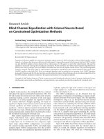
Figure 1: Illustration of filter decomposition for blind deconvolution.
where
F(z)
=
∞

r=0
F
r
z
−r
= H

(z)
L
1

p=1

1 − b
p
z

−1

−1
,
a

z
−1

=
∞

r=0
a
r
z
r
=
L
2

p=1
∞

q=0
d
−q
p
z
q

.
(8)
From the above analysis, we know that the demixing model
can be constructed by two parts: a causal filter F(z)andan
anticausal scalar filter a(z
−1
). The two subfilters can exchange
their positions because the filter a(z
−1
) is a scalar. As shown
in Figure 1 , we can obtain two decomposition forms as fol-
lows:
W(z)
= a

z
−1

F(z)orW(z) = F(z)a

z
−1

. (9)
In (8),
F
r
 and a
r
 decay exponentially to zero as r

tends to infinity. Hence, the decomposition of demixing filter
is reasonable. After being decomposed, we can use two one-
sided FIR filters to approximate filters F(z)anda(z
−1
)dueto
the decay properties of the coefficient of the inverse filter:
F(z)
=
N

p=0
F
p
z
−p
,
a

z
−1

=
N

p=0
a
p
z
p
,

(10)
where F
p
is an n × n-dimensional coefficientmatrixattime-
lag p, a
p
is a scalar at time-lag p,andN is a given positive
integer. This approximation w ill cause a model error in blind
decovolution. If we choose an appropriate fi lter length N,
the model error will become negligible and will not increase
computational cost.
3. LEARNING ALGORITHM
In the prev ious section, we decomposed the demixing filter
and introduced a new permutable cascade structure. To ob-
tain self-closed multiplication and inverse operations in the
manifold of FIR filters, we introduce some Lie Group’s prop-
erties. B ased on the geometrical structure of the FIR filter
manifold, the natural gradient algorithms are developed for
both subfilters.
3.1. Lie group
To discuss the geometrical property of FIR filter, we denote
the set of all one-sided FIR filters of length N as M(N):
M(N)
=

A(z) | A(z) =
N

p=0
A

p
z
−p

. (11)
In M(N), the operations of multiplication
∗ and inverse † are
defined as
A(z)
∗ B(z) =

A(z)B(z)

N
, (12)
where [
·]
N
is the truncating operator that any term with or-
der higher than N is omitted.
B
†
(z) =
N

p=0
B
†
p
z

−p
, (13)
where B
†
p
are recurrently defined by B
†
0
=B
−1
0
, B
†
1
=−B
†
0
B
1
B
†
0
,
B
†
p
=−

p
q

=1
B
†
p−q
B
q
B
†
0
, p = 1, , N.
For the sake of simplicity, we only give some properties
of Lie Group here. More detailed information can be found
in [20].
Property 1.
A(z)
∗

B(z) ∗ C(z)

=

A(z) ∗ B(z)

∗ C(z). (14)
4 EURASIP Journal on Advances in Signal Processing
Property 2.
B(z)
∗ B
†
(z) = B

†
(z) ∗ B(z) = I. (15)
Within the Lie group framework, the inverse F
†
(z) of the
causal filter F(z) still lies in the manifold M(N), w hile the
inverse a
†
(z
−1
) is in the same manifold with anticausal filter
a(z
−1
).
3.2. Learning algorithm
The purpose of blind deconvolution is to find an FIR demix-
ing filter W(z) such that the output of the demixing model
is maximally mutually independent and temporally i.i.d. The
Kullback-Leibler Divergence has been used as a criterion for
blind deconvolution [20, 24, 25] to measure the mutual in-
dependence of the output signals. In [20], the authors intro-
duced the following simple cost function for blind deconvo-
lution:
l

y, W(z)

=−
log



det

F
0



−
n

i=1
log p
i

y
i

, (16)
where the output signals y
i
={y
i
(k), k = 1, 2, }, i= 1, , n
is a stochastic process, p
i
(y
i
(k)) is the marginal probability
density function of y

i
(k)fori=1, , n and k = 1, , T,and
F
0
is an n × n-dimensional coefficient matrix at time-lag 0 of
filter F(z). The first term in the cost function is introduced to
prevent the matrix F
0
from being singular.
Using the cascade form in (9), we will develop the algo-
rithms for both F(z)anda(z
−1
). Here we introduce an inter-
mediate variable u,definedas
u(k)
=

a

z
−1

x(k),
y(k)
=

F(z)

u(k).
(17)

To calculate the natural gradient of the cost function, we con-
sider the differential of the cost function:
dl

y, W(z)

=−
d log


det

F
0



−
n

i=1
d log p
i

y
i

. (18)
Using the relation d log
| det(F

0
)|=tr(dF
0
F
−1
0
), we have
dl

y, W(z)

=−tr

dF
0
F
−1
0

+ ϕ(y)
T
dy, (19)
where ϕ(y)
= (ϕ
1
(y
1
), , ϕ
n
(y

n
))
T
is the vector of nonlinear
activation functions, defined by
ϕ
i

y
i

=−
d
dy
log

p
i

y
i

=−
p

i

y
i


p
i

y
i

,fori = 1, , n.
(20)
In order to develop the natural gradient algorithms for both
filters, we introduce nonholonomic transforms here:
dX(z)
= dF(z) ∗ F
†
(z),
db

z
−1

=
da

z
−1

∗
a
†

z

−1

.
(21)
In particular,
dX
0
= dF
0
F
−1
0
, (22)
da
0
= 0, db
0
= 0. (23)
Using the nonholonomic transforms, we c an easily calculate
dy(k)
= d

W(z)

x(k)
=

dF(z)a

z

−1

x(k)+

F(z)

da

z
−1

x(k)
=

dF(z) ∗ F
†
(z) ∗ F(z)

u(k)
+

F(z)da

z
−1

∗ a
†

z

−1

∗ a

z
−1

x(k)
=

dX(z)

y(k)+

db

z
−1

y(k).
(24)
Substituting (22)and(24) into (19), we have
dl

y, W(z)

=−
tr

dX

0

+ ϕ
T
(y)

dX(z)

y(k)
+ ϕ
T
(y)

db

z
−1

y(k).
(25)
Therefore, we obtain the derivatives of the cost function with
respect to X(z)andb(z
−1
)
∂l

y, W(z)

∂X
p

=−δ
0,p
I + ϕ

y(k)

y
T
(k − p),
∂l

y, W(z)

∂b
q
= ϕ
T

y(k)

y(k + q),
(26)
for p
= 0, 1, , N; q = 1, , N. The gradient descent algo-
rithms for X(z)andb(z
−1
)aregivenby
X
p
=−η

∂l

y, W(z)

∂X
p
= η

δ
0,p
I − ϕ

y(k)

y
T
(k − p)

,
b
q
=−η
∂l

y, W(z)

∂b
p
=−ηϕ
T


y(k)

y(k + q),
(27)
for p
= 0, 1, , N; q = 1, , N. Using the differential re-
lations (21), we derive learning algorithms for updating the
filters F(z)anda(z
−1
) as follows:
F(z) =X(z) ∗ F(z),
a

z
−1

=
b

z
−1

∗
a

z
−1

.

(28)
The learning algorithm can be written in the matrix form:
F
p
=−η
p

q=0
∂l

y, W(z)

∂X
p
F
p−q
= η
p

q=0

δ
0,q
I − ϕ

y(k)

y
T
(k − q)


F
p−q
,
a
p
=−η
p

q=0
∂l

y, W(z)

∂b
p
a
p−q
=−η
p

q=0

ϕ
T

y(k)

y(k + q)


a
p−q
(29)
B. Xia and L. Zhang 5
for p = 1, , N.In(29), there exists an unknown param-
eter ϕ, that is, the nonlinear activation function, which de-
pends on the probability density functions of the unknown
sources. According to the semiparameter theory, ϕ can be re-
garded as a nuisance parameter, therefore it is not necessary
to estimate it precisely. However, if we choose a better ϕ,it
is helpful for improving performance of the algorithm. For
example, a suitable activation function can greatly improve
the stability of the learning algorithm [20, 26].
4. COMPUTATIONAL COMPLEXITY AND
STABILITY CONDITIONS
As mentioned above, we use an anticausal scalar filter in new
cascade structure of demixing filter. It is not only to make the
structure permutable, but also to halve the computation re-
quirements. In [20], the demixing FIR filter was decomposed
into two one-sided FIR filters. If the order of the FIR filters
is N and the number of sensors is n,sowemustcompute
2
∗n
2
∗N parameters for each iteration. In the proposed algo-
rithm, we only need to compute n
2
∗N parameters for causal
FIRfilterandtocomputeN parameters for the scalar anti-
causal FIR filter at each iteration. So the computation cost is

lower than that in [20].
Amari et al. [26] derived the stability conditions for in-
stantaneous blind source separation. In [27], authors ana-
lyzed the stability of blind deconvolution and presented the
stability conditions. The proposed algorithms, developed by
using filter decomposition, are different from the algorithms
in [27]. So the stability conditions in [27] cannot be applied
directly to the algorithm developed for noncausal demixing
filters.
From (29) we know that the learning algorithms for up-
dating F
p
and a
p
, p = 0, 1, , N, are linear combination of
X
p
and b
p
, respectively. It is easy to see that the stability of X
p
and b
p
implies the stability of the learning algorithm. Here
we suppose that the estimated signals y
= (y
1
, , y
n
)

T
are
not only spatially mutually independent but also temporally
i.i.d.
The learning algorithms of X
p
and b
p
can be written as
follows:
dX
p
dt
= η

δ
0,p
I − ϕ

y(k)

y
T
(k − p)

,
db
p
dt
=−η


ϕ
T

y(k)

y(k + p)

,
(30)
where p
= 0, 1, , N. To analyze those asymptotic proper-
ties of the learning algorithms, we take expectation on the
above equations:
dX
p
dt
= η

δ
0,p
I − E

ϕ

y(k)

y
T
(k − p)


,
db
p
dt
=−η

E

ϕ
T

y(k)

y(k + p)

.
(31)
1
0
1
10 1
(a) Zero
1
0
1
10 1
(b) Pole
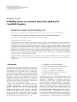
Figure 2: (a) Zero distributions of mixing model; (b) pole distr ibu-
tions of mixing model.

The stability conditions for (31) are obtained as follows:
k
i
> 0, for i = 1, , n,
k
i
k
j
σ
2
i
σ
2
j
> 1, for i, j = 1, , n,
m
i
+1> 0, for i = 1, , n,

i
k
i
σ
2
i
>

i

k

i
σ
2
i

−1
,
(32)
where m
i
= E[ϕ

(y
i
)y
2
i
], k
i
= E[ϕ

i
(y
i
)], σ
2
i
= E[|y
i
|

2
], i =
1, , n. Detailed derivation is left in the appendix.
5. SIMULATIONS
We now present several examples for simulating to illustrate
the performance of the proposed blind deconvolution algo-
rithm. The proposed algorithm is named as permutable fil-
ter decomposed method (PFD) and its performance is com-
pared with the decomposition method (FD) in [20] and the
natural gradient algorithm (NG) [5].Inthissection,wepro-
vide three simulation examples.
5.1. Separation experiment in nonminimum
phase system
In this simulation, we verify separation performance of the
proposed algorithm for nonminimum phase system. Here we
employ a mixing model generated by an ARMA model, de-
scribed as follows:
x(k)+
N

i=1
A
i
x(k − i) =
N

i=0
B
i
s(k − i)+v(k), (33)

where x(k) is the vector of mixing sig n als, s(k) is the vector of
source signals, and v(k) is the Gaussian noise with zero mean
and a covariance matr ix 0.1I. Using this ARMA model, we
can generate minimum phase or nonminimum phase mix-
ing model by choosing different A
i
and B
i
. From the dis-
tributions of zeros and poles shown in Figure 2, the mix-
ing system is stable and of nonminimum phase. The source
signals are three independent i.i.d. signals uniformly dis-
tributed in range (
−1, 1). The nonlinear activation function
6 EURASIP Journal on Advances in Signal Processing
1
0
1
050
G(z)
1,1
(a)
1
0
1
050
G(z)
1,2
(b)
1

0
1
050
G(z)
1,3
(c)
1
0
1
050
G(z)
2,1
(d)
1
0
1
050
G(z)
2,2
(e)
1
0
1
050
G(z)
2,3
(f)
1
0
1

050
G(z)
3,1
(g)
1
0
1
050
G(z)
3,2
(h)
1
0
1
050
G(z)
3,3
(i)
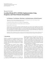
Figure 3: The coefficients of the global function at initiation.
is ϕ(y) = y
3
. We use batch method in this example to imple-
ment the proposed algorithm and the batch window is set as
6000. In the proposed algorithm, we use FIR filter to approx-
imate IIR filter, which will cause a model error. We should
choose an optimal filter length to minimize this model error.
In general, the MDL criterion is used to choose filter length
[20]. In this simulation, we set the filter length N as 20. The
initial learning r a te η is set to 0.01, and update learning rate
by η

= max{0.9η,10
−4
} for e very 10 iterations. As we defined
before, the G(z) is the global function whose coefficients ini-
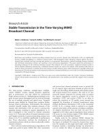
tial are show n in Figure 3. Generally, if the global function is
close to an identity filter, the source signals can be estimated
well. Figure 4 shows the coefficients of G(z) after conver-
gence. It is obvious that the G(z) is very close to an identity
filter. That means the proposed algorithm achieves good sep-
aration performance. Figures 5 and 6 show the coefficients of
the causal filter F(z) and the anticausal filter a(z
−1
), respec-
tively. The coefficients of both filters decay while the delay
number p increases.
5.2. Comparison of PFD, FD, and NG in
minimum phase system
The key point of filter decomposition method [20] is to di-
vide the nonminimum phase system into a minimum phase
part and a maximum part, and then use a causal filter and
an anticausal filter to demix the counterparts, respectively.
As shown in [20] and simulation 1, both PFD and FD work
well in nonminimum phase system. How about the perfor-
mance in minimum phase system? We compare the PFD, FD,
and NG [24] algorithms in minimum phase system here and
1
0
1
050
G(z)

1,1
(a)
1
0
1
050
G(z)
1,2
(b)
1
0
1
050
G(z)
1,3
(c)
1
0
1
050
G(z)
2,1
(d)
1
0
1
050
G(z)
2,2
(e)

1
0
1
050
G(z)
2,3
(f)
1
0
1
050
G(z)
3,1
(g)
1
0
1
050
G(z)
3,2
(h)
1
0
1
050
G(z)
3,3
(i)
Figure 4: The coefficients of the global function after convergence.
analyze the different performances of them.

We introduce the intersymbol interference as a perfor-
mance criterion. In [12, 28], the M
ISI
is defined as
M
ISI
=
n

i=1




n
j
=1

N
p
=−N


g
p,ij


−
max
p, j



g
p,ij





max
p, j


g
p,ij


+
n

j=1




n
i=1

N
p=−N



g
p,ij


−
max
p,i


g
p,ij





max
p,i


g
p,ij


.
(34)
In this simulation, we choose different A
i

and B
i
in (33)to
obtain a minimum phase mixing model. The source signals
in simulation 1 is used in this simulation. We set the filter
length of demixing filters and the learning rate update rule as
those in simulation 1 for three algorithms.
To remove the effect of a single numerical tr ial, we use
the ensemble average of 100 trails. Figure 7 illustrates the
comparison results of the three algorithms. It shows that the
performances of PFD and NG are similar, and both of them
are better than FD algorithm. That is because the FD algo-
rithm uses an er ror back propagation method to develop al-
gorithms for both subfilters. In the minimum phase system,
the anticausal filter should be an identity filter. But in FD
algorithm, the coefficients of anticausal filter did not achieve
the identity filter due to the error back propagation which de-
generates the convergence performance. In PFD algorithm,
there is not an error back propagation process. Therefore
PFD algorithm can obtain the same performance with nat-
ural gradient algorithm.
B. Xia and L. Zhang 7
1
0
1
01020
(z)
1,1
(a)
1

0
1
01020
(z)
1,2
(b)
1
0
1
01020
(z)
1,3
(c)
1
0
1
01020
(z)
2,1
(d)
1
0
1
01020
(z)
2,2
(e)
1
0
1

01020
(z)
2,3
(f)
1
0
1
01020
(z)
3,1
(g)
1
0
1
01020
(z)
3,2
(h)
1
0
1
01020
(z)
3,3
(i)
Figure 5: Coefficients of F(z).
0.6
0.4
0.2
0

0.2
0.4
0.6
0.8
1
0 5 10 15 20 25
Figure 6: Coefficients of a(z
−1
).
5.3. Comparison of PFD and FD in the
nonminimum phase system
We intend to compare the proposed algorithm with other
algorithms in nonminimum phase system. But some algo-
rithms cannot work well in the situation of simulation 1,
such as NG algorithm and Bussgang algorithm. In this sim-
ulation, we only compared PFD and FD algorithms in non-
minimum phase system because both algorithms can sepa-
rate mixing signals. The coefficients of mixing filter H(z)are
set the same as experiment 1. We set the filter length N to 20
at both sides. Figure 8 shows the 100 trails ensemble average
comparison result. The PFD algorithm converges faster than
FD. B ecause the computational cost is lower in PFD at each
10
1
10
0
10
1
10
2

0 50 100 150 200 250 300
NG
FD
PFD
M
ISI
Figure 7: Comparison results of M
ISI
in minimum phase system.
10
1
10
0
10
1
10
2
0 50 100 150 200 250 300
FD
PFD
M
ISI
Figure 8: Comparison results of M
ISI
in nonminimum phase sys-
tem.
iteration than in FD. During the computing, we find the M
ISI
fluctuates at the initiation in FD algorithm due to the error
back propagation. In PFD algorithm, we use scalar anticausal

filter in PFD and then avoid the error back propagation. So
the convergence processing is smooth.
6. CONCLUSION
In this paper we present a permutable cascade form for
multichannel blind deconvolution in nonminimum phase
system. By decomposing the demixing anticausal FIR filter
into two sub-FIR filters, the difficult problem is divided into
several easy subtasks. The structure of demixing model is
permutable because an anticausal scalar FIR filter is used.
8 EURASIP Journal on Advances in Signal Processing
Natural gra dient-based algorithms can be easily developed
for two one-sided filters. Using the permutable charac teristic
of this cascade structure, we derive the stability conditions
for the proposed algorithm. Finally, the simulation results
show the efficiency and performance of the proposed algo-
rithm.
APPENDIX
In this appendix, we provide the detailed derivation for the
stability conditions. The learning algorithms for updating F
k
and a
k
, k = 0, 1, , N, are linear combination of X
k
and b
k
,
respectively. T he stability of X
k
and b

k
implies the stability
of the learning algorithm. Here we suppose that the separat-
ing signals y
= (y
1
, , y
n
)
T
are not only spatially mutually
independent but also temporally i.i.d.
Consider (31), if the variational matrix at equilibrium
point is negative definite, then the system is stable in the
vicinity of the equilibrium point. Taking a variation δX
p
on
X
p
and a variation δb
p
on b
p
,respectively,wehave
dδX
p
dt
=−ηE

ϕ



y(k)

δyy
T
(k − p)+ϕ

y(k)

δy
T
(k − p)

,
dδb
p
dt
=−ηE

ϕ


y(k)

T
δy(k)y(k + p)
+ ϕ
T


y(k)

δy(k + p)

.
(A.1)
Furthermore, we write the differential expression of
δy(k)
δy(k)
=

a(z)δF(z)+δa(z)F(z)

x(k)
=

δX(z)+Iδb(z)

y(k).
(A.2)
As mentioned above, the mat rix F
0
is nonsingular. This
means that the learning algorithms keep the filters F(z)and
a(z) on the same manifold with the initial filter. This prop-
erty implies that the equilibrium point of the learning algo-
rithm satisfies the following equations:
E

I − ϕ


y(k)

y
T
(k)

=
0. (A.3)
Using the mutual independence and i.i.d. properties of
the output signals y
i
, i = 1, , n and the normalized condi-
tion (A.3), we deduce (A.1)to
dδX
p
dt
=−ηE

ϕ


y(k)

δX(z)

+ Iδb(z)y(k)

y
T

(k − p)
+ ϕ

y(k)

y
T
(k − p)

δX(z)+δb(z)

T

,
dδb
p
dt
=−ηE

ϕ


y(k)

T

δX(z)+δb(z) ∗ I

y(k)y(k + p)
+ ϕ

T

y(k)

δX(z)+δb(z) ∗ I

y(k + p)

.
(A.4)
When p
= 0,
dδX
0
dt
=−ηE

ϕ


y(k)

δX
0
y(k)y
T
(k)+ϕ

y(k)


y
T
(k)δX
T
0

,
(A.5)
dδb
0
dt
= 0. (A.6)
Rewrite (A.5) in component form
dδX
0,ij
dt
=−η

k
i
σ
2
j
δX
0,ij
+ δX
0, ji

,
dδX

0, ji
dt
=−η

k
j
σ
2
i
δX
0, ji
+ δX
0,ij

,
(A.7)
for i
= j,and
dδX
0,ii
dt
=−η

m
i
+1

δX
0,ii
,(A.8)

for p
= 1, , N,andi, j = 1, , n,wherem
i
= E[ϕ

(y
i
)y
2
i
],
k
i
= E[ϕ

i
(y
i
)], σ
2
i
= E[|y
i
|
2
], i = 1, , n. The stability con-
ditions of (A.7)and(A.8)aregivenby
k
i
> 0, for i = 1, , n,

k
i
k
j
σ
2
i
σ
2
j
> 1, for i, j = 1, , n,
m
i
+1> 0, for i = 1, , n.
(A.9)
When p
= 0
dδX
p
dt
=−ηE

ϕ


y(k)

δX
p
y(k − p)y

T
(k − p)
+ ϕ

y(k)

δb
p
y
T
(k)

=−
η

kIδX
p
σ
2
+ δb
p
I

,
(A.10)
dδb
p
dt
=−ηE


ϕ


y(k)

T
δb
p
y
T
(k + q)y(k + q)
+ ϕ
T

y(k)

δX
p
y(k)

=−
η


i
k
i
σ
2
i

δb
p
+

i
δX
p,ii

.
(A.11)
For i
= j, the components form of (A.10)canberewrit-
ten as follows:
dδX
p
dt
=−η

k
i
σ
2
j
δX
p,ij

. (A.12)
The stability condition for (A.12) is as follows:
k
i

> 0, for i = 1, , n. (A.13)
From (A.11), we know that only the diagonal entries of
δX
p
are relative with δb
p
,fori = j. The diagonal component
form of δX
p
can be written as
dδX
p,ii
dt
=−η

k
i
σ
2
i
δX
p,ii
+ δb
p

. (A.14)
B. Xia and L. Zhang 9
Combining (A.11)and(A.14), we get
d
dt

⎡
⎢
⎢
⎢
⎢
⎣
δX
p,11
.
.
.
δX
p,nn
δb
p
⎤
⎥
⎥
⎥
⎥
⎦
=−
η
⎡
⎢
⎢
⎢
⎢
⎢
⎣

k
1
σ
2
1
0 ··· 1
.
.
.
.
.
.
···
.
.
.
0
··· k
n
σ
2
n
1
1
··· 1

i
k
i
σ

2
i
⎤
⎥
⎥
⎥
⎥
⎥
⎦
⎡
⎢
⎢
⎢
⎢
⎣
δX
p,11
.
.
.
δX
p,nn
δb
p
⎤
⎥
⎥
⎥
⎥
⎦

.
(A.15)
If we want to make the variation matrix be negative, we
should let

i
k
i
σ
2
i
−

i

k
i
σ
2
i

−1
> 0. (A.16)
So we obtain the stability condition for p
= 0

i
k
i
σ

2
i
>

i

k
i
σ
2
i

−1
,fori = 1, , n. (A.17)
In summary, we have the total stability conditions for the
natural gradient algorithm of the blind deconvolution as fol-
lows:
k
i
> 0, for i = 1, , n,
k
i
k
j
σ
2
i
σ
2
j

> 1, for i, j = 1, , n,
m
i
+1> 0, for i = 1, , n,

i
k
i
σ
2
i
>

i

k
i
σ
2
i

−1
.
(A.18)
ACKNOWLEDGMENTS
The work was supported by the National Basic Research Pro-
gram of China (Grant no. 2005CB724301) and National Nat-
ural Science Foundation of China (Grant no. 60375015).
REFERENCES
[1] S. Amari, “Natural gradient works efficiently in learning,”

Neural Computation, vol. 10, no. 2, pp. 251–276, 1998.
[2] A. J. Bell and T. J. Sejnowski, “An information-maximization
approach to blind separation and blind deconvolution,” Neu-
ral Computation, vol. 7, no. 6, pp. 1129–1159, 1995.
[3] J F. Cardoso and B. Laheld, “Equivariant adaptive source sep-
aration,” IEEE Transactions on Signal Processing, vol. 44, no. 12,
pp. 3017–3030, 1996.
[4] P. Comon, “Independent component analysis: a new con-
cept?” Signal Processing, vol. 36, no. 3, pp. 287–314, 1994.
[5] S. Amar i, S. Douglas, A. Cichocki, and H. Yang, “Novel on-line
algorithms for blind deconvolution using natural gradient ap-
proach,” in Proceedings of the 11th IFAC Symposium on System
Identification (SYSID ’97), pp. 1057–1062, Kitakyushu, Japan,
July 1997.
[6] S. Bellini, “Bussgang techniques for blind equalization,” in
Proceedings of IEEE Global Telecommunications Conference
(GLOBECOM ’86), pp. 1634–1640, Houston, Tex, USA, De-
cember 1986.
[7] A. Benveniste, M. Goursat, and G. Ruget, “Robust identifica-
tion of a nonminimum phase system: blind adjustment of a
linear equalizer in data communications,” IEEE Transactions
on Automatic Control, vol. 25, no. 3, pp. 385–399, 1980.
[8] D. N. Godard, “Self-recovering equalization and carrier track-
ing in two-dimensional data communication systems,” IEEE
Transactions on Communications Systems, vol. 28, no. 11, pp.
1867–1875, 1980.
[9] Y. Hua, “Fast maximum likelihood for blind identification of
multiple FIR channels,” IEEE Transactions on Signal Processing,
vol. 44, no. 3, pp. 661–672, 1996.
[10] O. Shalvi and E. Weinstein, “New criteria for blind deconvolu-

tion of nonminimum phase systems (channels),” IEEE Trans-
actions on Informat ion Theory, vol. 36, no. 2, pp. 312–321,
1990.
[11] L. Tong, G. Xu, and T. Kailath, “Blind identification and equal-
ization based on second-order statistics: a time domain ap-
proach,” IEEE Transactions on Information Theory, vol. 40,
no. 2, pp. 340–349, 1994.
[12] J. K. Tugnait, “Channel estimation and equalization using
high-order statistics,” in Signal Processing Advances in Wireless
and Mobile Communications, G. B. Giannakis, Y. Hua, P. Sto-
ica, and L. Tong, Eds., vol. 1, pp. 1–40, Prentice-Hall, Upper
Saddle River, NJ, USA, 2000.
[13] J. K. Tugnait and B. Huang, “Multistep linear predictors-
based blind identification and equalization of multiple-input
multiple-output channels,” IEEE Transactions on Signal Pro-
cessing, vol. 48, no. 1, pp. 26–38, 2000.
[14] Y. Li, A. Cichocki, and L. Zhang, “Blind source estimation
of FIR channels for binary sources: a grouping decision ap-
proach,” Signal Processing, vol. 84, no. 12, pp. 2245–2263, 2004.
[15] S. Amari, A. Cichocki, and H. H. Yang, “A new learning algo-
rithm for blind signal separation,” in Advances in Neural Infor-
mation Processing Systems. Vol. 8 (NIPS ’95),D.S.Touretzky,
M. C. Mozer, and M. E. Hasselmo, Eds., pp. 757–763, MIT
Press, Cambridge, Mass, USA, 1996.
[16] S. C. Douglas, “Simplified plant estimation for multichan-
nel active noise control,” in Proceedings of 18th International
Congress on Acoustics (ICA ’ 04), Kyoto, Japan, April 2004.
[17] J. Labat, O. Macchi, and C. Laot, “Adaptive decision feedback
equalization: can you skip the training period?” IEEE Transac-
tions on Communications, vol. 46, no. 7, pp. 921–930, 1998.

[18] L Q. Zhang, A. Cichocki, and S. Amari, “Multichannel blind
deconvolution of nonminimum phase systems using informa-
tion backpropagation,” in Proceedings of the 6th International
Conference on Neural Information Processing (ICONIP ’99),pp.
210–216, Perth, Australia, November 1999.
[19] K. Waheed and F. M. Salam, “Cascaded structures for blind
source recovery,” in
Proceedings of the 45th IEEE International
Midwest Symposium on Circuits and Systems (MSCAS ’02),
vol. 3, pp. 656–659, Tulsa, Okla, USA, August 2002.
[20] L Q. Zhang, A. Cichocki, and S. Amari, “Multichannel blind
deconvolution of nonminimum-phase systems using filter de-
composition,” IEEE Transactions on Signal Processing, vol. 52,
no. 5, pp. 1430–1442, 2004.
[21] A. Hyv
¨
arinen, J. Karhunen, and E. Oja, Independent Compo-
nent Analysis, John Wiley & Sons, New York, NY, USA, 2001.
[22] S. Haykin, Unsupervised Adaptive Filtering, Volume 2: Blind
Deconvolution, John Wiley & Sons, New York, NY, USA, 2000.
[23] A. K. Nandi and S. N. Anfinsen, “Blind equalization with re-
cursive filter structures,” Signal Processing, vol. 80, no. 10, pp.
2151–2167, 2000.
[24] S. Amari, S. C. Doug las, A. Cichocki, and H. H. Yang, “Mul-
tichannel blind deconvolution and equalization using the nat-
ural gradient,” in Proceedings of the 1st IEEE Signal Processing
Workshop on Signal Processing Advances in Wireless Communi-
cations (SPAWC ’97), pp. 101–104, Paris, France, April 1997.
10 EURASIP Journal on Advances in Signal Processing
[25] D. T. Pham, “Mutual information approach to blind separa-

tion of stationary sources,” IEEE Transactions on Information
Theory, vol. 48, no. 7, pp. 1935–1946, 2002.
[26] S. Amari, T P. Chen, and A. Cichocki, “Stability analysis of
learning algorithms for blind source separation,” Neural Net-
works, vol. 10, no. 8, pp. 1345–1351, 1997.
[27] L Q. Zhang, A. Cichocki, and S. Amari, “Geometrical struc-
tures of FIR manifold and multichannel blind deconvolution,”
The Journal of VLSI Signal Processing, vol. 31, no. 1, pp. 31–44,
2002.
[28] Y. Inouye and S. Ohno, “Adaptive algorithms for implement-
ing the single-stage criterion for multichannel blind deconvo-
lution,” in Proceedings of the 5th International Conference on
Neural Information Processing (ICONIP ’98), pp. 733–736, Ki-
takyushu, Japan, October 1998.
Bin Xia received his B.S. degree in mechan-
ical engineering from Luoyang Institute of
Technology, in 1997, and M.S. degree in me-
chanical engineering from Guizhou Univer-
sity, China, in 2001. He is currently a Ph.D.
candidate of Department of Computer Sci-
ences and Engineering, Shanghai Jiao Tong
University, China. His research interests in-
clude statistical signal processing, blind sig-
nal processing, and machine learning.
Liqing Zhang received his B.S. degree in
mathematics from Hangzhou University, in
1983, and the Ph.D. degree in computer sci-
ences from Zhongshan University, China, in
1988. He became an Associate Professor in
1990 and then a Full Professor in 1995 at the

Department of Automation, South China
University of Technology. He joined Labo-
ratory for Advanced Brain Signal Process-
ing, RIKEN Brain Science Institute, Japan,
in 1997 as a Research Scientist. Since 2002, he has been working
in Department of Computer Sciences and Engineering, Shanghai
Jiao Tong University, China. His research interests include neuroin-
formatics, perception computing, adaptive systems, and statistical
learning. He has published more than 110 papers.