Hindawi Publishing Corporation
EURASIP Journal on Advances in Signal Processing
Volume 2008, Article ID 765462, 11 pages
doi:10.1155/2008/765462
Research Article
Blind Channel Equalization Using Constrained Generalized
Pattern Search Optimization and Reinitialization Strategy
Abdelouahib Zaouche,
1
Iyad Day oub,
2
Jean Michel Rouvaen,
2
and Charles Tatkeu
1
1
INRETS LEOST, 20 rue Elisee Reclus, 59650 Villeneuve d’Ascq, France
2
IEMN DOAE, University of Valenciennes and Hainaut-Cambresis, Le Mont Houy, 59313 Valenciennes, France
Correspondence should be addressed to Abdelouahib Zaouche,
Received 5 November 2007; Revised 28 May 2008; Accepted 26 August 2008
Recommended by William Sandham
We propose a global convergence baud-spaced blind equalization method in this paper. This method is based on the application
of both generalized pattern optimization and channel surfing reinitialization. The potentially used unimodal cost function relies
on higher- order statistics, and its optimization is achieved using a pattern search algorithm. Since the convergence to the global
minimum is not unconditionally warranted, we make use of channel surfing reinitialization (CSR) strategy to find the right global
minimum. The proposed algorithm is analyzed, and simulation results using a severe frequency selective propagation channel are
given. Detailed comparisons with constant modulus algorithm (CMA) are highlighted. The proposed algorithm performances
are evaluated in terms of intersymbol interference, normalized received signal constellations, and root mean square error vector
magnitude. In case of nonconstant modulus input signals, our algorithm outperforms significantly CMA algorithm with full
channel surfing reinitialization strategy. However, comparable performances are obtained for constant modulus signals.

Copyright © 2008 Abdelouahib Zaouche et al. This is an open access article distributed under the Creative Commons Attribution
License, which permits unrestricted use, distribution, and reproduction in any medium, provided the original work is properly
cited.
1. INTRODUCTION
The major problem encountered in digital communications
is intersymbol interference (ISI). The received signal is
seriously distorted, due to the band limiting effect of
the channel and the multipath propagation phenomenon.
To overcome such problems, various channel equalization
techniques have been proposed over the past few years.
Most of these techniques take advantage of known training
sequences to adaptively extract channel information. The
main drawback with this approach is bandwidth consuming
due to training. To overcome this resource wasting, blind
equalization algorithms have been proposed. In this case,
instead of using training sequences, only input signal and
noise statistical properties are required. Thus, the original
transmitted message is recovered from the received sequence
that is corrupted by noise and ISI with no training sequence
nor a priori channel knowledge [1]. In general, the blind
equalization techniques can be classified according to their
signals statistical properties exploitation, as those using
maximum likelihood (ML) methods [2], or second-order
statistics (SOS) [3] or higher-order statistics (HOS) [1,
4]. The latter include inverse filter criteria-(IFC-) based
algorithms [5], the super exponential algorithm (SEA) [6],
polyspectra-based algorithm [7], and Bussgang algorithms
[8]. Blind equalization based on higher-order statistics relies
mainly on the optimization of nonlinear and nonconvex cost
functions. These cost functions have a highly multimodal

geometrical structure with many local minima [9, 10].
This fact makes the global optimization task very tedious.
Nowadays many digital communication schemes transmit
constant modulus (CM) signals. Hence, several iterative-
gradient-based blind equalization algorithms exploiting this
precious information, namely, the constant modulus crite-
rion, have been developed and have gained a widespread
use in different communication systems [9]. Among these
algorithms, the constant modulus algorithm (CMA) is the
most commonly used. Moreover, it is reputed to be the
simplest and most successful HOS-based blind equalization
algorithm [4, 9, 10]. However, the multimodal structure of
the nonconvex and nonlinear CM fitness function makes
these algorithms extremely vulnerable to converge toward
local minima. This leads to formulate the problem of blind
equalization as a constrained gradient-free optimization
2 EURASIP Journal on Advances in Signal Processing
+
s
k
c
k
n
k
y
k
w
k
z
k

g
Channel Equalizer
Channel-equalizer
Figure 1: Block diagram of the system.
problem using generalized pattern search algorithm that
minimizes
g
4
2
−g
4
4
over a search space, where g is the
joint channel-equalizer impulse response. This cost function
is known to be potentially unimodal as discussed in [11, 12];
however, this is not sufficient to warrant global convergence.
To overcome this limitation and to ensure good global
convergence behavior, we propose to use the channel surfing
reinitialization strategy to estimate the optimal delay.
2. SYSTEM MODEL
The block diagram of the system under consideration is
shown in Figure 1. It represents a single-input-single-output
(SISO) channel equalizer. The source sequence
{s
k
},with
finite real or complex alphabet, is assumed to be sub-
Gaussian (kurtosis < 3ifrealorkurtosis< 2ifcomplex),
circular (E
{s

2
k
}=0 in the complex case), independent, and
identically distributed (i.i.d) with variance E
{|s
k
|
2
}=σ
2
s
.
This sequence is transmitted through a complex linear time
invariant baseband channel represented by a discrete finite
impulse response (FIR) filter c of length P as
c
=

c
0
c
1
··· c
P−1

T
,(1)
the c
k
’s being complex numbers.

The resulting signal is corrupted by a zero-mean random
Gaussian noise
{n
k
} with variance σ
2
n
, independent of
the input source sequence
{s
k
}, resulting in the regressor
sequence
{y
k
}. The latter is then processed by an L-taped FIR
blind equalizer with complex coefficients w,givenby
w
=

w
0
w
1
··· w
L−1

T
. (2)
The goal of the blind equalizer is to provide an accurate

estimate of the transmitted sequence, that we denote by
{z
k
}. This is achieved when the combined channel-equalizer
impulse response g
= c ⊗ w (⊗ meaning convolution)
behaves as a simple delay operator resulting in
{z
k
}≈{s
k−δ
}.
This is referred to as the zero forcing condition which can be
measured using the intersymbol interference (ISI) formula
defined in terms of the global channel-equalizer taps as
ISI
=
(

i
|g
i
|
2
) −|g|
2
max
|g|
2
max

,(3)
where
|g|
max
stands for the maximum joint channel-
equalizer filter weight in absolute value.
Furthermore, it can be noticed that the zero forcing
condition corresponds ideally to an ISI equal to zero. Thus,
blind equalization can be viewed as the minimization of the
above ISI.
3. PROBLEM FORMULATION
Most of blind equalization algorithms rely on the minimiza-
tion of nonconvex cost functions. Among these algorithms,
constant modulus algorithm (CMA) is the most commonly
used blind equalization scheme. It is mainly based on the use
of stochastic gradient descent (SGD) strategy to minimize
the nonconvex Godard’s cost function defined by J
= E{(γ −
|
z
k
|
2
)
2
},whereγ = E{|s
k
|
4
}/E{|s

k
|
2
} is the dispersion
constant [13, 14]. However, the use of such nonconvex cost
functions may result in undesirable convergence problems
due to the presence of several local minima and saddle
points. To overcome this limitation, many zero forcing
blind equalization cost functions have been proposed in the
literature [12–15]. In this paper, we use one of them, which is
simple in implementation and gives the best performances.
This cost function is expressed in terms of joint channel
equalizer impulse response as
g
4
2
−g
4
4
=


i


g
i


2


2
−

i


g
i


4
. (4)
It has been shown in [13, 14] that by employing the gradient
of the cost function with respect to g
i
and setting it to zero,
the corresponding extrema are the solutions of the following
equation:


i


g
i


2
−



g
i


2

g
i
= 0. (5)
Note that (5) has two different solutions, one of which cor-
responds to g
= 0. This undesirable solution may be avoided
by imposing a linear constraint on the equalizer weights.
Among the linear constraints proposed in the literature, we
can cite the normalization of the blind equalizer weights
w

= w/
√
w
H
w after each iteration or, as suggested in [16],
the assessment of a linear constraint of the form
u
T
w = e with u
/
=0, e

/
=0. (6)
However, in order to reduce the computation complexity and
to avoid the division by zero, here we use a linear constraint.
This latter consists in setting one tap of the blind equalizer
(say at index δ) to zero. This is formulated as
minimize f (w)
=g
4
2
−g
4
4
subject to w
δ
= 1, (7)
where 0
≤ δ ≤ L − 1.
The second solution of (5) corresponds to the desired
zero forcing condition in which at most one nonzero element
Abdelouahib Zaouche et al. 3
The current
point
(a)
The current
point
(b)
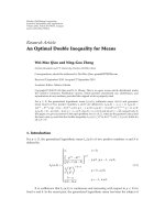
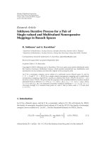
Figure 2:Patternvectorsforthe(a)GPS2N = 4 positive basis and
(b) GPS N +1
= 3 positive basis.

of the joint channel-equalizer impulse response g is allowed
and the remaining taps are ideally forced to zeros. The use
of a linear constraint on the equalizer tap directly rather
than on g is due to two factors. The first one concerns the
unavailability of g. The second factor is motivated by the
direct relationship between maximizing one tap of g located
at any position δ and maximizing the equalizer tap located at
the same position.
As discussed in [12], in the case of baud-spaced equal-
ization (BSE), the cost function
g
4
2
−g
4
4
is sectionally
convex in g and unimodal both in g and w for infinite length
equalizers (L
=∞). Moreover, in most practical situations
corresponding to BSE with finite N, the optimization
problem of (7) is a unimodal one in g for a given delay
δ and potentially unimodal in w. Thus, unimodality in
w, which ensures a global convergence, is not necessarily
obtained. Unimodality in w for finite length BSE remains still
unproven.
Godard’s cost function has many local minima and
saddle points for a given delay. Since the proposed cost
function has a unique minimum in g for a given delay, it is
less likely to have many local minima in w, unlike Godard’s.

However, the problem of global convergence still rises. Thus,
in order to overcome this limitation, we propose to use the
channel surfing reinitialization (CSR) strategy suggested in
[17]. This has been originally proposed for CMA and we
suggest to adapt here to the blind optimization problem of
(7). CSR consists of varying the delay index δ systematically
and searching the optimum equalizer w for each delay
value. Finally, the optimum index which minimizes the cost
function f (w) is retained. In fact, unlike the CSR-CMA,
where the algorithm parameters (step size and maximum
number of iterations) must be adjusted for each value of δ
to insure convergence, we propose to use CSR only to predict
the global optimal delay index δ
†
for the blind equalizer tap
which is fixed to one. First, for the sake of simplicity, we
introduce a notation for the shift operator applied on any
given vector u as
SHIFT
K,n
(u)
Δ
= u(n − K), (8)
where K is an integer delay.
Let us also define the covariance matrix estimate of the
preequalized data sequence
{y
k
} as


R
Δ
= E

y
k
y
H
k

. (9)
As discussed in [17–19], if a Wiener equalizer for a particular
delay has a reasonably good mean square error (MSE) per-
formance in estimating
{s
k−δ
}, there exists a blind equalizer
in its immediate neighborhood. Using the converged blind
equalizer w
δ
as an estimate of the MMSE equalizer results
in the following estimate of the unknown channel impulse
response [17, 18]:
c =

Rw
δ
. (10)
A performance measure of the blind equalizer after conver-
gence is the following estimate of the Wiener cost function:


J = 1 −w
H
δ
c = 1 −w
H
δ

Rw
δ
. (11)
The optimal delay is found using
δ
†
= arg min
⎧
⎪
⎨
⎪
⎩
1 −


R
−1
SHIFT
δ,k
(c)

H

SHIFT
δ,k
(c)
  

J
δ,k
⎫
⎪
⎬
⎪
⎭
. (12)
Therefore, the local optimization problem of (7)istrans-
formed into the global blind equalization problem stated as
minimize f (w)
=g
4
2
−g
4
4
subject to w
δ
†
= 1.
(13)
It can be noticed that the optimization problem shown
above is formulated in terms of the unknown joint channel-
equalizer impulse response g. Consequently, its implemen-

tation requires the formulation of the cost function only
in terms of known quantities. These latter are the blind
equalizer output sequence
{z
k
} and the corresponding
statistical measures related to the input source sequence
{s
k
}.
It has been previously shown in [11] that
f (w)
=

E{|z
k
|
2
}
E{|s
k
|
2
}

2
−
E{|z
k
|

4
}−3(E{|z
k
|
2
})
2
E{|s
k
|
4
}−3(E{|s
k
|
2
})
2
. (14)
Using the definitions for the variance σ
2
s
and the
normalized kurtosis κ
s
of the source sequence {s
k
}:
σ
2
s

 E



s
k


2

, κ
s

E
{|s
k
|
4
}
σ
4
s
, (15)
and those for the equalizer output statistics:
E



z
k



2

=
1
N
N

k=1


z
k


2
, E



z
k


4

=
1
N

N

k=1


z
k


4
, (16)
where N is the length of the sequence
{z
k
},(14)maybe
written as
f (w)
=
ξκ
s
N
2

N

k=1


z
k



2

2
−
ξ
N

N

k=1


z
k


4

, (17)
where ξ
= 1/(κ
s
−3)σ
4
s
.
4 EURASIP Journal on Advances in Signal Processing
10.80.60.40.20

Normalized frequency/π
−10
−5
0
5
10
Magnitude (dB)
10.80.60.40.20
Normalized frequency/π
−200
−100
0
100
Phase (degrees)
(a)
10−1−2−3
Real part
−1.5
−1
−0.5
0
0.5
1
1.5
Imaginary part
(b)
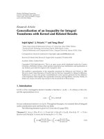
Figure 3: Example channel characteristics: (a) (top) frequency response, (a) (bottom) phase response, (b) and zeroes locations.
2520151050
Optimal delay
Delay index

Wiener equalizers
CSR with
||g||
4
2
−||g||
4
4
−1.5
−1
−0.5
0
0.5
1
MSE
(a)
2520151050
Optimal delay
Delay index
Wiener equalizers
10
−2
10
−1
10
0
MSE (log scale)
(b)
Figure 4: MSE versus system delays for (a) Wiener equalizers and logarithmic view for (b) Wiener equalizers.
Considering the digital communication system of

Figure 1, the equalizer output z
k
can be expressed in terms of
the unknown blind equalizer vector and the known regressor
vector as
z
k
= w
H
y
k
. (18)
Substituting (18) into (17) yields the desired formulation
of the cost function in terms only of the unknown blind
equalizer vector and known statistical quantities as depicted
below:
f (w)
=
ξκ
s
N
2

N

k=1


w
H

y
k


2

2
−
ξ
N

N

k=1


w
H
y
k


4

. (19)
The proposed cost function deals with both real and complex
channels and equalizers. In fact, the unknown blind equalizer
is given by
w
= w

real
+ jw
img
. (20)
The effect of using complex equalizers rather than real ones
resides in doubling the number of the unknown variables to
be found by the optimization process.
Finally, in order to solve the optimization problem, the
expression for f (w)of(19) must now be substituted into
(13).
The following section is dedicated to solving the above
constrained optimization problem using generalized pattern
search algorithm.
Abdelouahib Zaouche et al. 5
4035302520151050
SNR (dB)
100 samples
500 samples
1000 samples
1500 samples
2000 samples
Wiener
−35
−30
−25
−20
−15
−10
−5
0

5
ISI (dB)
Figure 5: The proposed algorithm ISI performance for different
sample sequence lengths and SNRs.
4035302520151050
SNR (dB)
CMA0
CMA1
CMA4
Wiener
−35
−30
−25
−20
−15
−10
−5
0
ISI (dB)
Figure 6: CMA ISI performance for different single spike initializa-
tions and SNRs.
4. BACKGROUND ON GENERALIZED PATTERN
SEARCH ALGORITHM
Generalized pattern search (GPS) algorithms that were first
defined and analyzed by Torczon [20] for derivative-free
unconstrained optimization belong to the family of direct
search methods. In fact they rely on searching for a set of
points around the current point, forming a mesh, in order
to find one fitness value lower than that at the current
point. The essence of defining a mesh is to find a set of

positive spanning directions D in R
n
.Tobetterunderstand
the notion of positive spanning, we introduce the following
definitions and terminology thanks to Davids [21].
Definition 1. A positive combination of the set of vectors D
=
{
d
i
}
r
i
=1
is a linear combination

r
i
=1
α
i
d
i
,whereα
i
≥ 0, i =
1, 2, , r.
Definition 2. A finite set of vectors D
={d
i

}
r
i
=1
forms
a positive spanning set for R
n
,ifeveryv ∈ R
n
can be
expressed as a positive combination of vectors in D. The set
of vectors D is said to positively span R
n
. The set D is said to
be a positive basis for R
n
if no proper subset of D positively
spans R
n
.
Davids demonstrated a very important feature, which
proves determinant in the choice of the set of positive
direction in GPS algorithms, namely, the cardinal of any
positive set D in R
n
,thatwedenoteasm,liesbetweenn +1
and 2n. This is mathematically formulated as
n +1
≤ m = card(D) ≤ 2n, (21)
where the lower limit n +1andupperlimit2n stand for

the cardinals of the minimal and maximal positive bases,
respectively.
It is common to choose the positive bases as the columns
of D
max
= [I
n×n
, −I
n×n
]orD
min
= [I
n×n
, −e
n×1
], where I
n×n
is the n × n identity matrix and e
n×1
is the n-dimensional
column vector of ones [22, 23]. As an example to highlight
this point, let us consider that the blind equalization problem
formulated using (13) is a two-dimensional one. This means
that the unknown equalizer vector w has two taps (n
= 2).
According to (21), the cardinal of the positive basis to be used
while applying GPS algorithm to the optimization problem
lies between 3 and 4. Indeed, the corresponding minimal
positive basis having a cardinal of 3 is constructed of the
column vectors of the matrix:

D
min
=

I
2×2
, −e
2×1

=

10−1
01
−1

, (22)
yielding the following pattern search vectors:
d
1
=

10

T
, d
2
=

01


T
, d
3
=

−
1 −1

T
.
(23)
Moreover, the corresponding maximal positive basis D
max
is
then constructed as
D
max
=

I
2×2
, −I
2×2

=

10−10
01 0
−1


, (24)
yielding
d
1
=

10

T
,
d
2
=

01

T
,
d
3
=

−
10

T
,
d
4
=


0 −1

T
.
(25)
6 EURASIP Journal on Advances in Signal Processing
3210−1−2−3
Real
−3
−2
−1
0
1
2
3
Imaginary
(a)
10.50−0.5−1
Real
−1
−0.5
0
0.5
1
Imaginary
(b)
10.50−0.5−1
Real
−1

−0.5
0
0.5
1
Imaginary
(c)
10.50−0.5−1
Real
−1
−0.5
0
0.5
1
Imaginary
(d)
Figure 7: (a) QPSK constellations before equalization, (b) after equalization using GPS, (c) after equalization using CMA0, and (d) after
equalization using CMA1.
These two minimal and maximal positive bases corre-
sponding to the 2-dimensional optimization problem are
illustrated in Figure 2. It is very important to point out the
fact that the previous method of choosing the set of positive
spanning directions is not unique.
In fact there is a great freedom in choosing these
directions, but the set of positive directions D can be always
expressed under the form [24, 25]
[D]
n×m
= [G]
n×n
[Z]

n×m
, (26)
where G is a nonsingular real generating matrix (most often
taken as the identity matrix) and Z is a full rank integer
matrix. Therefore, each direction vector d
j
∈ D can be
expressed as d
j
= Gz
j
,wherez
j
is an integer vector of length
n.
5. BLIND EQUALIZATION USING GPS ALGORITHM
Generalized pattern search algorithms consist mainly of two
phases: an optional search step and a local poll step. In
Abdelouahib Zaouche et al. 7
1.510.50−0.5−1−1.5
Real
−1.5
−1
−0.5
0
0.5
1
1.5
Imaginary
(a)

1.510.50−0.5−1−1.5
Real
−1.5
−1
−0.5
0
0.5
1
1.5
Imaginary
(b)
Figure 8: 4-PAM constellations after equalization using (a) GPS or (b) CMA2.
1.510.50−0.5−1−1.5
Real
−1.5
−1
−0.5
0
0.5
1
1.5
Imaginary
(a)
10.50−0.5−1
Real
−1
−0.5
0
0.5
1

Imaginary
(b)
Figure 9: 16-QAM constellations after equalization using (a) GPS or (b) CMA2.
fact, the search step relies on the exploration of a large
number of mesh points around the current point which is
computational and time consuming. This phase is therefore
omitted in the present work. On the contrary, the local poll
step only explores the neighborhood of the current iteration
on the mesh. This set of points P
k
is called the poll set and is
defined by [24–26]
P
k
=

w
k
+ Δ
k
d
k
: d
k
∈ D
k
⊆ D

, (27)
where Δ

k
> 0 is the mesh size parameter that controls the
fitness of the mesh, w
k
the current kth blind equalizer vector
and D
k
is a positive spanning set of directions d
k
taken from
D.
At iteration k, in order to find some point belonging to
P
k
where the inequality f (w
k
+Δ
k
d
k
) <f(w
k
) is verified, the
poll phase is carried out by evaluating the fitness function
that we need to optimize (namely, f ) around the current
blind equalizer vector w
k
.Ifsuchanimprovedmeshpoint
8 EURASIP Journal on Advances in Signal Processing
10987654321

Index value
QPSK
16-QAM
4-PAM
0.1
0.11
0.12
0.13
0.14
0.15
0.16
0.17
Root mean square EVM
Figure 10: Averaged r.m.s. EVM values for CMA with various spike
initializations.
(that decreases the fitness value) is found, then the iteration k
is called successful; otherwise it is considered unsuccessful. If
the iteration is successful, the improved mesh point becomes
the new iterate. This is achieved by setting w
k+1
= w
k
+Δ
k
d
k
.
In this case, the mesh size parameter Δ
k
is increased using the

following updating rule:
Δ
k+1
= min

τΔ
k
, Δ
max

, (28)
where τ>1isastepincreasefactor(oftentakenequalto2),
Δ
0
is the initial step size, and Δ
max
is the maximum step size.
The min(
·) function is used to ensure an upper limit to step
size expansion.
On the other side, if no improved mesh point is found in
all the poll step around P
k
, the vector w
k
is said to be a mesh
local optimizer and is retained as the new iterate w
k+1
= w
k

.
Moreover, the mesh size parameter decreases following the
equation:
Δ
k+1
= max

Δ
k
τ
, Δ
min

, (29)
where the max(
·) function ensures that the exploration step
does not get lower than a minimum step size Δ
min
.
The process is repeated until a suitable stopping criterion
is satisfied (maximum number of iterations exceeded or step
size lower than the tolerance limit). The GPS algorithm is
summarized in Algorithm 1 [27, 28].
6. SIMULATION RESULTS
The validity of the proposed method has been studied using
simulation. We consider the, assumed unknown, real baud
spaced channel:
c
=


0.4, 1, −0.7, 0.6, 0.3, −0.4, 0.1

T
, (30)
which is the same channel used in [6].
Initialization
choose an initial guess
w for w
set minimal value of step for convergence test Δ
tol
> 0
set maximal value of step Δ
max
> Δ
tol
> 0
set initial step value Δ
0
(Δ
max
> Δ
0
> Δ
tol
)
set maximal iteration count k max
init iteration count k to 0
define the set of positive directions D
Main loop
loop:

if k
≤ k
max
then
compute values of cost function on neighboring points
if there exists d
l
∈ D such that
f (w
k
+ Δ
k
d
l
) <f(w
k
) then
set w
k+1
= w
k
+ Δ
k
d
k
set Δ
k+1
= min(τΔ
k
, Δ

max
)
if Δ
k+1
< Δ
max
increment k
go to loop
else
exit loop
else
set w
k+1
= w
k
set Δ
k+1
= max(Δ
k
/τ,Δ
min
)
if Δ
k+1
> Δ
min
increment k
go to loop
else
exit loop

else exit loop
Algorithm 1: The algorithm for GPS optimization.
The corresponding magnitude and phase versus fre-
quency characteristics, together with the z-plane zero pat-
tern, are plotted in Figure 3. Note that the magnitude
frequency response of this channel undergoes one severe
fading (see Figure 3(a) top) and its corresponding phase is
nonlinear (see Figure 3(a) bottom). Moreover this channel is
mixed phase with four zeros inside the unit circle and one
outside as highlighted in Figure 3(b).
We start by applying the GPS algorithm to the con-
strained blind equalization problem depicted in (7). The
used input sequence is an i.i.d. unit power quadrature phase
shift keying (QPSK) signal with a length of 2000 samples and
the simulation parameters are as follows: the signal to noise
ratio (SNR) is set to 20 dB, the blind equalizer is a FIR baud
spaced equalizer of length L
= 20, Δ
0
= 1 (initial step size),
Δ
min
= 10
−7
, Δ
max
= 10
7
, τ = 2. The value of τ taken here
is the most often used in the literature and its only effect

is to speed up or slow down convergence. The step related
values play the role of stopping criteria: the min insures
the precision of the converged value, the max alleviates fast
divergence problems and the initial must take a reasonable
value intermediate between both previous ones. Moreover, a
maximum number of iterations has been fixed to 500, a value
Abdelouahib Zaouche et al. 9
Table 1: Minimal cost using GPS for different delays around
optimum.
Delay index Cost Delay index Cost
2 −1.2513 3 −1.2703
4
−1.2755 5 −1.2743
6
−1.2717 7 −1.2711
which has been sufficient for most tries we performed on a
number of different channels.
Since the selection of the fixed tap location is strictly
related to the optimal delay selection problem and, assuming
no a priori channel knowledge, we choose a linear constraint
that fixes some tap to one at each iteration.
The probably suboptimal blind equalizer obtained after
convergence is then used to estimate the desired optimal
delay position using the CSR strategy as expressed in (12).
Figure 4(a) shows the simulated estimates of the Wiener cost
function for different delays from 0 to 25. Let us note that
this exceeds the equalizer filter length (taken equal to 20),
but enables us to verify that a sufficiently high value has been
chosen for it.
In Figure 4(a), the theoretical Wiener equalizer based on

minimum square error (MSE) is given for the same delay
positions. Let us remember that the MSE is defined as
MSE
Δ
= E



z
k
−s
k−δ


2

, (31)
and its corresponding optimal vector minimizer, namely, the
Wiener equalizer is found as [13]
w
†
=

C
H
C +
σ
2
n
σ

2
s
C
H
g
δ
†

−1
C
H
g
δ
†
, (32)
where C is the baud channel convolution matrix and δ
†
represents the desired optimal delay index, which corre-
sponds to the index of the minimum diagonal element of
I
−C(C
H
C + σ
2
n
I/σ
2
s
)
−1

C
H
.
It can be easily noticed from Figure 4(a) that both graphs
have the same trend thus allowing the selection of the
optimal delay which corresponds to an index δ
†
= 4.
The value of the optimal delay is more clearly evidenced
in Figure 4(b), which presents essentially the same data
as Figure 4(a) for the MSE optimal equalizers, but in
logarithmic scale. However, due to the occurrence of negative
values for the simulated estimates of the Wiener cost function
in Figure 4(a), full logarithmic representation is not truly
feasible. Thus, the exact simulated values are given in Tabl e 1
for index values around the optimum δ
†
.
The negative values found for the Wiener cost function
estimates result from the imposed blind equalizer linear
constraint that fixes one tap to one. In fact, the zero forcing
joint channel-equalizer impulse response has its important
tap situated exactly at that position where the coefficient is
constrained to be one. This results in w
δ
c > 1in(11). The
negative values are not then to be considered as reflecting
better performances in comparison to the theoretical Wiener
MSE, but quite the contrary. It is actually more evident
from Ta ble 1 that the estimated lowest cost value of

−1.2755
corresponds to a delay index δ
†
= 4. This latter is in
accordance with the theoretical Wiener optimal delay δ
†
.At
present time, the constrained blind equalization problem can
be reformulated more accurately as
minimize f (w) subject to w
δ
†
= w
4
= 1. (33)
We apply GPS algorithm to this global optimization problem
under the same simulation parameters (just stated above)
but for different values of SNRs and different regressor
sequence lengths N. The measured performance will be the
intersymbol interference ISI, redefined below in logarithmic
scale (dB values) as
ISI(dB)
Δ
= 10 log
10

[

i
|g

i
|
2
] −|g|
2
max
|g|
2
max

. (34)
Each simulation is run 30 times and the corresponding
averaged results values are given in Figure 5.Itcanbenoticed
that the global blind equalization performs well for values
of N
≥ 1000 and is comparable to the Wiener equalizer for
N
= 2000.
For performance comparison with the constant
modulus algorithm, we use the BERGulator software
for CMA simulations which may be downloaded from
Figure 6 shows the
CMA simulated performances in terms of ISI for different
SNR values and three single spike initialization strategies,
that we denote by CMA0, CMA1, and CMA4 the numerical
values 0, 1, and 4 standing for the index of the unique
nonzero blind equalizer tap in the initialization vector. The
simulation parameters, the modulation type, the unknown
channel, and the blind equalizer length, are the same as
before; the fixed step size is μ

= 5 × 10
−4
and the iteration
number is set to 2
×10
4
to ensure final convergence.
It can be easily seen that, unlike the proposed algorithm
which ensures global convergence behavior for sufficient
samples sequence length, CMA is extremely vulnerable to
the way of selecting the initial blind equalizer vector and
local convergence is more likely to happen. This latter point
is clearly highlighted in the case of CMA0 and CMA1.
Moreover, the optimal Wiener delay index (which is in
our case 4) corresponds exactly to the optimal position of
the non-null element of CMA4 initial vector and also to
the position of the equalizer tap constrained to one in the
proposed algorithm. It may be noticed that CSR may equally
well be applied to CMA, with the result of selecting the
CMA4 case after initialization.
Furthermore, the proposed global blind optimization-
based algorithm outperforms significantly CMA in terms of
local convergence properties and gives slightly better global
performance than CMA4 (that is also CMA with CSR),
especially in low-noise environments (SNR
≥ 30 dB).
Figure 7 represents the constellations obtained for QPSK
modulation, with SNR
= 20 dB at receiver input. Let us
notice that these constellations have been normalized, the

baseband received signal modulus being taken as unity.
It is clearly seen that the constellations points are not
10 EURASIP Journal on Advances in Signal Processing
Table 2: Averaged r.m.s. EVM values using the proposed algorithm
and CMA with optimum delay index δ
†
, for three modulation
types.
Modulation type GPS Optimum CMA
QPSK 0.1090 0.1094
16-QAM 0.1243 0.1339
4-PAM 0.0997 0.1181
resolved before equalization and become distinguishable for
CMA0 and more separated for CMA1. A constellation phase
rotation effect may also be noticed for CMA0 and, to a lesser
extent, CMA1. Very satisfactory results are obtained with
our proposed algorithm using GPS, these for CMA4 being
visually quite identical. In fact, one approaches the Wiener
optimumsolutioninbothcases.
Other modulation types have been investigated. Figures
8 and 9 show constellations (normalized such that the
baseband signal power is equal to unity) obtained for,
respectively, 4-level pulse amplitude modulation (4-PAM)
and 16-level quadrature amplitude modulation (16-QAM).
Only results from our GPS-based algorithm (a little
better than those obtained with CMA4) and with CMA2
are shown for comparison purposes (constellations before
equalization and using a CMA1 equalizer are not shown
here).
The good performance of our algorithm is again evi-

denced. It may be noticed that, as may be logically expected,
the same value is obtained for δ
†
independently of the
modulation type.
Apart from constellation rotation, a measure of the
equalizer efficiency is obtained using error vector magnitude
(EVM) [29, 30]. The root mean square (r.m.s.) EVM is
defined as
EVM
=





N
i=1
(ΔI
2
i
+ ΔQ
2
i
)
N

N
i=1
(I

2
0,i
+ Q
2
0,i
)
, (35)
where N is the number of emitted symbols, I
0,i
and Q
0,i
,are
the inphase and quadrature components, respectively, of the
reference (noiseless) signal, ΔI
i
= I
i
−I
0,i
, ΔQ
i
= Q
i
−Q
0,i
, I
i
and Q
i
being the inphase and quadrature components of the

received (noisy) signals.
Our algorithm has been run 30 times on sequences of
2000 emitted QPSK, 16-QAM, or 4-PAM symbols and 2000
added noise samples with 20 dB SNR, to get the averaged
r.m.s. EVM values given in Ta b le 2 (the averaging process
is taken over a sufficiently high number of samples as per
Monte Carlo method).
The simulation has been repeated using CMA and
variable spike initializations for comparison purposes. The
EVM results are shown in Figure 10 versus delay index value
around optimum (from 1 to 10) for the three previously used
modulation types.
The corresponding minimum cost function values (for
delay index δ
†
) are also given in Tab le 2 .
Not surprisingly, one sees that the performance decreases
for higher efficiency 16-QAM modulation. Moreover 4-PAM
and 16-QAM are not constant envelope modulations and
thus CMA is not well-suited for them. As a consequence, our
GPS-based algorithm outperforms noticeably CMA in these
two cases. It has also been noticed during the simulation that
our algorithm gives much lesser dispersion in EVM values
when compared to CMA (lower variance).
7. DISCUSSION AND CONCLUSION
In this paper, a baud spaced blind equalization method based
on GPS and CSR has been presented in detail and compared
to the CMA algorithm. Successful simulation results have
been obtained on a number of different, real, or complex
channels. For example, real static channel presenting a single

deep fading and mixed phase has been presented. We have
shown the good performances of the proposed equalizer,
even for nonconstant envelope modulations. For constant
envelope modulations, the performances are nearly identical
to that given by CMA, after selecting the optimum CMA
spike delay value for its initialization vector and correctly
choosing its step size. This has also been verified for QPSK as
reported here and noted for 8-PSK and 16-PSK. Other static
channels with more than one fading have also been tested,
with essentially the same conclusions as above.
Our algorithm involves unavoidable steps of cost func-
tion computation (as any other equalization one) and simple
algebraic equations for updating the equalizer weights (no
gradient computation), testing, and loop instructions. It
may be implemented in a FPGA-floating point DSP struc-
ture, owing to its reasonable complexity. For performance
evaluation, the main concern is the number of required
cost function evaluations (which depends on the speed
of convergence, and thus equalized channel and initial
conditions). The comparison with CMA algorithm using
CSR initialization, for a number of different channels,
leads to the conclusion that the number of cost function
evaluations is of the same order of magnitude as the CSR-
CMA and our algorithm, with a little to significant advantage
for the latter in the cases of channels with problems
(like amplitude or frequency selectivity) or of nonconstant
modulus modulations.
Our future work will be directed to extending our
algorithm to fractionally spaced equalization, improving the
CSR step, and using space diversity. Moreover, the case of

slowly varying channels will be considered.
ACKNOWLEDGMENT
The authors thank Dr. Walaa Hamouda from the Depart-
ment of Electrical and Computer Engineering of Concordia
University for helpful comments and suggestions that have
ledtoanimprovedpaper.
REFERENCES
[1] J. Zhu, X R. Cao, and R W. Liu, “A blind fractionally spaced
equalizer using higher order statistics,” IEEE Transactions on
Circuits and Systems II, vol. 46, no. 6, pp. 755–764, 1999.
Abdelouahib Zaouche et al. 11
[2] F. Alberge, P. Duhamel, and M. Nikolova, “Adaptive solution
for blind identification/equalization using deterministic max-
imum likelihood,” IEEE Transactions on Signal Processing, vol.
50, no. 4, pp. 923–936, 2002.
[3] J P. Delmas, H. Gazzah, A. P. Liavas, and P. A. Regalia,
“Statistical analysis of some second-order methods for blind
channel identification/equalization with respect to channel
undermodeling,” IEEE Transactions on Signal Processing, vol.
48, no. 7, pp. 1984–1998, 2000.
[4] C Y. Chi, C Y. Chen, C H. Chen, and C C. Feng, “Batch
processing algorithms for blind equalization using higher-
order statistics,” IEEE Signal Processing Magazine, vol. 20, no.
1, pp. 25–49, 2003.
[5] C H. Chen, C Y. Chi, and W T. Chen, “New cumulant-based
inverse filler criteria for deconvolution of nonminimum phase
systems,” IEEE Transactions on Signal Processing, vol. 44, no. 5,
pp. 1292–1297, 1996.
[6] M. Kawamoto, M. Ohata, K. Kohno, Y. Inouye, and A. K.
Nandi, “Robust super-exponential methods for blind equal-

ization in the presence of Gaussian noise,” IEEE Transactions
on Circuits and Systems II: Express Briefs, vol. 52, no. 10, pp.
651–655, 2005.
[7] A.G. Bessios and C. L. Nikias, “POTEA: the power cepstrum
and tricoherence equalization algorithm,” IEEE Transactions
on Communications, vol. 43, no. 11, pp. 2667–2671, 1995.
[8] H. Mathis and S. C. Douglas, “Bussgang blind deconvolution
for impulsive signals,” IEEE Transactions on Signal Processing,
vol. 51, no. 7, pp. 1905–1915, 2003.
[9] B. Maricic, Z Q. Luo, and T. N. Davidson, “Blind constant
modulus equalization via convex optimization,” IEEE Trans-
actions on Signal Processing, vol. 51, no. 3, pp. 805–818, 2003.
[10] R. Pandey, “Complex-valued neural networks for blind equal-
ization of time varying channels,” International Journal of
Signal Processing, vol. 1, no. 1, pp. 1–8, 2005.
[11] V. Shtrom and H. Fan, “A refined class of cost functions in
blind equalization,” in Proceedings of the IEEE International
Conference on Acoustics, Speech, and Signal Processing (ICASSP
’97), vol. 3, pp. 2273–2276, Munich, Germany, April 1997.
[12] V. Shtrom and H. Fan, “New class of zero-forcing cost
functions in blind equalization,” IEEE Transactions on Signal
Processing, vol. 46, no. 10, pp. 2674–2683, 1998.
[13] C. R. Johnson Jr., P. Schniter, T. J. Endres, J. D. Behm, D. R.
Brown, and R. A. Casas, “Blind equalization using the constant
modulus criterion: a review,” Proceedings of the IEEE, vol. 86,
no. 10, pp. 1927–1950, 1998.
[14] S. Chen, T. B. Cook, and L. C. Anderson, “A comparative study
of two blind FIR equalizers,” DigitalSignalProcessing, vol. 14,
no. 1, pp. 18–36, 2004.
[15] S. Vembu, S. Verdu, R. A. Kennedy, and W. Sethares, “Convex

cost functions in blind equalization,” IEEE Transactions on
Signal Processing, vol. 42, no. 8, pp. 1952–1960, 1994.
[16] A. T. Erdogan and C. Kizilkale, “Fast and low complexity blind
equalization via subgradient projections,” IEEE Transactions
on Signal Processing, vol. 53, no. 7, pp. 2513–2524, 2005.
[17] L. Tong and H. H. Zeng, “Channel surfing reinitialization
for the constant modulus algorithm,” IEEE Signal Processing
Letters, vol. 4, no. 3, pp. 85–87, 1997.
[18] S. Evans and L. Tong, “Online adaptive reinitialization of
the constant modulus algorithm,” IEEE Transactions on Signal
Processing, vol. 48, no. 4, pp. 537–539, 2000.
[19] H. H. Zeng, L. Tong, and C. R. Johnson Jr., “Relationships
between the constant modulus and wiener receivers,” IEEE
Transactions on Information Theory, vol. 44, no. 4, pp. 1523–
1538, 1998.
[20] V. Torczon, “On the convergence of pattern search algo-
rithms,” SIAM Journal on Optimization
, vol. 7, no. 1, pp. 1–25,
1997.
[21] C. Davids, “Theory of positive linear dependence,” American
Journal of Mathematics, vol. 76, no. 4, pp. 733–746, 1954.
[22] E. Polak and M. Wetter, “Generalized pattern search algo-
rithms with adaptive precision function evaluations,” Tech.
Rep. LBNL-52629, Lawrence Berkeley National Laboratory,
Berkeley Calif, USA, May 2003.
[23] E. D. Dolan, R. M. Lewis, and V. Torczon, “On the local
convergence of pattern search,” SIAM Journal on Optimization,
vol. 14, no. 2, pp. 567–583, 2003.
[24] M. A. Abramson, “Second-order behavior of pattern search,”
SIAM Journal on Optimization, vol. 16, no. 2, pp. 515–530,

2006.
[25] C. Audet and J. E. Dennis Jr., “A pattern search filter
method for nonlinear programming without derivatives,”
SIAM Journal on Optimization, vol. 14, no. 4, pp. 980–1010,
2004.
[26] M. A. Abramson, C. Audet, and J. E. Dennis Jr., “Generalized
pattern searches with derivative information,” Mathematical
Programming, vol. 100, no. 1, pp. 3–25, 2004.
[27] A. Zaouche, I. Dayoub, and J. M. Rouvaen, “Blind constant
modulus equalization using hybrid genetic algorithm and
pattern search optimization,” in Proceedings of the 7th World
Wireless Congress (WWC ’06), pp. 37–42, San Francisco, Calif,
USA, May 2006.
[28] A. Zaouche, I. Dayoub, and J. M. Rouvaen, “Blind equalization
via the use of generalized pattern search optimization and
zero forcing sectionnally convex cost function,” in Proceedings
of the 2nd IEEE International Conference on Information and
Communication Technologies (ICTTA ’06), vol. 2, pp. 2303–
2308, Damaskus, Syria, April 2006.
[29] K. M. Voelker, “Apply error vector measurements in commu-
nications design,” Microwaves & RF, pp. 143–152, December
1995.
[30] R. Hassun, M. Flaherty, R. Matreci, and M. Taylor, “Effective
evaluation of link quality using error vector magnitude tech-
niques,” in Proceedings of the Annual Wireless Communications
Conference, pp. 89–94, Boulder, Calif, USA, August 1997.