Constrution
of exact
two-sided
confidence
intervals
based on the
binomial
distribution
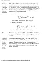
If the number of failures is very small or if the sample size N is very
small, symmetical confidence limits that are approximated using the
normal distribution may not be accurate enough for some applications.
An exact method based on the binomial distribution is shown next. To
construct a two-sided confidence interval at the 100(1 -
)% confidence
level for the true proportion defective p where N
d
defects are found in a
sample of size N follow the steps below.
Solve the equation
for p
U
to obtain the upper 100(1 - )% limit for p.
1.
Next solve the equation
for p
L
to obtain the lower 100(1 - )% limit for p.
2.
Note The interval {p
L
, p

U
} is an exact 100(1 - )% confidence interval for p.
However, it is not symmetric about the observed proportion defective,
.
Example of
calculation
of upper
limit for
binomial
confidence
intervals
using
EXCEL
The equations above that determine p
L
and p
U
can easily be solved
using functions built into EXCEL. Take as an example the situation
where twenty units are sampled from a continuous production line and
four items are found to be defective. The proportion defective is
estimated to be
= 4/20 = 0.20. The calculation of a 90% confidence
interval for the true proportion defective, p, is demonstrated using
EXCEL spreadsheets.
7.2.4.1. Confidence intervals
(3 of 9) [5/1/2006 10:38:37 AM]
Upper
confidence
limit from

EXCEL
To solve for p
U
:
Open an EXCEL spreadsheet and put the starting value of 0.5 in
the A1 cell.
1.
Put =BINOMDIST(Nd, N, A1, TRUE) in B1, where Nd = 4 and N
= 20.
2.
Open the Tools menu and click on GOAL SEEK. The GOAL
SEEK box requires 3 entries./li>
B1 in the "Set Cell" box
❍
/2 = 0.05 in the "To Value" box❍
A1 in the "By Changing Cell" box.❍
The picture below shows the steps in the procedure.
3.
Final step Click OK in the GOAL SEEK box. The number in A1 will
change from 0.5 to P
U
. The picture below shows the final result.
4.
7.2.4.1. Confidence intervals
(4 of 9) [5/1/2006 10:38:37 AM]
Example of
calculation
of lower
limit for
binomial

confidence
limits using
EXCEL
The calculation of the lower limit is similar. To solve for p
L
:
Open an EXCEL spreadsheet and put the starting value of 0.5 in
the A1 cell.
1.
Put =BINOMDIST(Nd -1, N, A1, TRUE) in B1, where Nd -1 = 3
and N = 20.
2.
Open the Tools menu and click on GOAL SEEK. The GOAL
SEEK box requires 3 entries.
B1 in the "Set Cell" box
❍
1 - /2 = 1 - 0.05 = 0.95 in the "To Value" box❍
A1 in the "By Changing Cell" box.❍
The picture below shows the steps in the procedure.
3.
7.2.4.1. Confidence intervals
(5 of 9) [5/1/2006 10:38:37 AM]
Final step Click OK in the GOAL SEEK box. The number in A1 will
change from 0.5 to p
L
. The picture below shows the final result.
4.
7.2.4.1. Confidence intervals
(6 of 9) [5/1/2006 10:38:37 AM]
Interpretation

of result
A 90% confidence interval for the proportion defective, p, is {0.071,
0.400}. Whether or not the interval is truly "exact" depends on the
software. Notice in the screens above that GOAL SEEK is not able to
find upper and lower limits that correspond to exact 0.05 and 0.95
confidence levels; the calculations are correct to two significant digits
which is probably sufficient for confidence intervals. The calculations
using a package called SEMSTAT agree with the EXCEL results to
two significant digits.
Calculations
using
SEMSTAT
The downloadable software package SEMSTAT contains a menu item
"Hypothesis Testing and Confidence Intervals." Selecting this item
brings up another menu that contains "Confidence Limits on Binomial
Parameter." This option can be used to calculate binomial confidence
limits as shown in the screen shot below.
7.2.4.1. Confidence intervals
(7 of 9) [5/1/2006 10:38:37 AM]
Calculations
using
Dataplot
This computation can also be performed using the following Dataplot
program.
. Initalize
let p = 0.5
let nd = 4
let n = 20
. Define the functions
let function fu = bincdf(4,p,20) - 0.05

let function fl = bincdf(3,p,20) - 0.95
. Calculate the roots
let pu = roots fu wrt p for p = .01 .99
let pl = roots fl wrt p for p = .01 .99
. print the results
let pu1 = pu(1)
let pl1 = pl(1)
print "PU = ^pu1"
print "PL = ^pl1"
Dataplot generated the following results.
PU = 0.401029
PL = 0.071354
7.2.4.1. Confidence intervals
(8 of 9) [5/1/2006 10:38:37 AM]
7.2.4.1. Confidence intervals
(9 of 9) [5/1/2006 10:38:37 AM]
7. Product and Process Comparisons
7.2. Comparisons based on data from one process
7.2.4. Does the proportion of defectives meet requirements?
7.2.4.2.Sample sizes required
Derivation of
formula for
required
sample size
when testing
proportions
The method of determining sample sizes for testing proportions is similar
to the method for determining sample sizes for testing the mean.
Although the sampling distribution for proportions actually follows a
binomial distribution, the normal approximation is used for this

derivation.
Minimum
sample size
If we are interested in detecting a change in the proportion defective of
size
in either direction, the minimum sample size is
For a two-sided test
1.
For a one-sided test2.
Interpretation
and sample
size for high
probability of
detecting a
change
This requirement on the sample size only guarantees that a change of size
is detected with 50% probability. The derivation of the sample size
when we are interested in protecting against a change with probability
1 -
(where is small) is
For a two-sided test
1.
For a one-sided test2.
7.2.4.2. Sample sizes required
(1 of 2) [5/1/2006 10:38:38 AM]
where is the upper critical value from the normal distribution that is
exceeded with probability
.
Value for the
true

proportion
defective
The equations above require that p be known. Usually, this is not the
case. If we are interested in detecting a change relative to an historical or
hypothesized value, this value is taken as the value of p for this purpose.
Note that taking the value of the proportion defective to be 0.5 leads to
the largest possible sample size.
Example of
calculating
sample size
for testing
proportion
defective
Suppose that a department manager needs to be able to detect any change
above 0.10 in the current proportion defective of his product line, which
is running at approximately 10% defective. He is interested in a one-sided
test and does not want to stop the line except when the process has clearly
degraded and, therefore, he chooses a significance level for the test of
5%. Suppose, also, that he is willing to take a risk of 10% of failing to
detect a change of this magnitude. With these criteria:
z
.05
= 1.645; z
.10
=1.2821.
= 0.102.
p = 0.103.
and the minimum sample size for a one-sided test procedure is
7.2.4.2. Sample sizes required
(2 of 2) [5/1/2006 10:38:38 AM]

7. Product and Process Comparisons
7.2. Comparisons based on data from one process
7.2.5.Does the defect density meet
requirements?
Testing defect
densities is
based on the
Poisson
distribution
The number of defects observed in an area of size A units is often
assumed to have a Poisson distribution with parameter A x D, where D
is the actual process defect density (D is defects per unit area). In other
words:
The questions of primary interest for quality control are:
Is the defect density within prescribed limits?1.
Is the defect density less than a prescribed limit?2.
Is the defect density greater than a prescribed limit?3.
Normal
approximation
to the Poisson
We assume that AD is large enough so that the normal approximation
to the Poisson applies (in other words, AD > 10 for a reasonable
approximation and AD > 20 for a good one). That translates to
where is the standard normal distribution function.
Test statistic
based on a
normal
approximation
If, for a sample of area A with a defect density target of D
0

, a defect
count of C is observed, then the test statistic
can be used exactly as shown in the discussion of the test statistic for
fraction defectives in the preceding section.
7.2.5. Does the defect density meet requirements?
(1 of 3) [5/1/2006 10:38:44 AM]
Testing the
hypothesis
that the
process defect
density is less
than or equal
to D
0
For example, after choosing a sample size of area A (see below for
sample size calculation) we can reject that the process defect density is
less than or equal to the target D
0
if the number of defects C in the
sample is greater than C
A
, where
and Z is the upper 100x(1- ) percentile of the standard normal
distribution. The test significance level is 100x(1-
). For a 90%
significance level use Z
= 1.282 and for a 95% test use Z = 1.645.
is the maximum risk that an acceptable process with a defect
density at least as low as D
0

"fails" the test.
Choice of
sample size
(or area) to
examine for
defects
In order to determine a suitable area A to examine for defects, you first
need to choose an unacceptable defect density level. Call this
unacceptable defect density D
1
= kD
0
, where k > 1.
We want to have a probability of less than or equal to
is of
"passing" the test (and not rejecting the hypothesis that the true level is
D
0
or better) when, in fact, the true defect level is D
1
or worse.
Typically
will be .2, .1 or .05. Then we need to count defects in a
sample size of area A, where A is equal to
Example Suppose the target is D
0
= 4 defects per wafer and we want to verify a
new process meets that target. We choose
= .1 to be the chance of
failing the test if the new process is as good as D

0
( = the Type I
error probability or the "producer's risk") and we choose
= .1 for the
chance of passing the test if the new process is as bad as 6 defects per
wafer ( = the Type II error probability or the "consumer's risk").
That means Z = 1.282 and Z
1-
= -1.282.
The sample size needed is A wafers, where
7.2.5. Does the defect density meet requirements?
(2 of 3) [5/1/2006 10:38:44 AM]
which we round up to 9.
The test criteria is to "accept" that the new process meets target unless
the number of defects in the sample of 9 wafers exceeds
In other words, the reject criteria for the test of the new process is 44
or more defects in the sample of 9 wafers.
Note: Technically, all we can say if we run this test and end up not
rejecting is that we do not have statistically significant evidence that
the new process exceeds target. However, the way we chose the
sample size for this test assures us we most likely would have had
statistically significant evidence for rejection if the process had been
as bad as 1.5 times the target.
7.2.5. Does the defect density meet requirements?
(3 of 3) [5/1/2006 10:38:44 AM]
7. Product and Process Comparisons
7.2. Comparisons based on data from one process
7.2.6.What intervals contain a fixed
percentage of the population values?
Observations

tend to
cluster
around the
median or
mean
Empirical studies have demonstrated that it is typical for a large
number of the observations in any study to cluster near the median. In
right-skewed data this clustering takes place to the left of (i.e., below)
the median and in left-skewed data the observations tend to cluster to
the right (i.e., above) the median. In symmetrical data, where the
median and the mean are the same, the observations tend to distribute
equally around these measures of central tendency.
Various
methods
Several types of intervals about the mean that contain a large
percentage of the population values are discussed in this section.
Approximate intervals that contain most of the population values●
Percentiles●
Tolerance intervals for a normal distribution●
Tolerance intervals using EXCEL●
Tolerance intervals based on the smallest and largest
observations
●
7.2.6. What intervals contain a fixed percentage of the population values?
[5/1/2006 10:38:44 AM]
7. Product and Process Comparisons
7.2. Comparisons based on data from one process
7.2.6. What intervals contain a fixed percentage of the population values?
7.2.6.1.Approximate intervals that contain
most of the population values

Empirical
intervals
A rule of thumb is that where there is no evidence of significant
skewness or clustering, two out of every three observations (67%)
should be contained within a distance of one standard deviation of the
mean; 90% to 95% of the observations should be contained within a
distance of two standard deviations of the mean; 99-100% should be
contained within a distance of three standard deviations. This rule can
help identify outliers in the data.
Intervals
that apply to
any
distribution
The Bienayme-Chebyshev rule states that regardless of how the data
are distributed, the percentage of observations that are contained within
a distance of
k tandard deviations of the mean is at least (1 -
1/k
2
)100%.
Exact
intervals for
the normal
distribution
The Bienayme-Chebyshev rule is conservative because it applies to any
distribution. For a normal distribution, a higher percentage of the
observations are contained within
k standard deviations of the mean as
shown in the following table.
Percentage of observations contained between the mean and k

standard deviations
k, No. of
Standard
Deviations
Empircal Rule Bienayme-Chebychev
Normal
Distribution
1 67% N/A 68.26%
2 90-95% at least 75% 95.44%
3 99-100% at least 88.89% 99.73%
4 N/A at least 93.75% 99.99%
7.2.6.1. Approximate intervals that contain most of the population values
(1 of 2) [5/1/2006 10:38:45 AM]