Process or Product Monitoring and Control_6 ppt
Bạn đang xem bản rút gọn của tài liệu. Xem và tải ngay bản đầy đủ của tài liệu tại đây (1.12 MB, 22 trang )
Table
showing
squared
error for the
mean for
sample data
Next we will examine the mean to see how well it predicts net income
over time.
The next table gives the income before taxes of a PC manufacturer
between 1985 and 1994.
Year $ (millions) Mean Error
Squared
Error
1985 46.163 48.776 -2.613 6.828
1986 46.998 48.776 -1.778 3.161
1987 47.816 48.776 -0.960 0.922
1988 48.311 48.776 -0.465 0.216
1989 48.758 48.776 -0.018 0.000
1990 49.164 48.776 0.388 0.151
1991 49.548 48.776 0.772 0.596
1992 48.915 48.776 1.139 1.297
1993 50.315 48.776 1.539 2.369
1994 50.768 48.776 1.992 3.968
The MSE = 1.9508.
The mean is
not a good
estimator
when there
are trends
The question arises: can we use the mean to forecast income if we
suspect a trend? A look at the graph below shows clearly that we should
not do this.
6.4.2. What are Moving Average or Smoothing Techniques?
(3 of 4) [5/1/2006 10:35:07 AM]
Average
weighs all
past
observations
equally
In summary, we state that
The "simple" average or mean of all past observations is only a
useful estimate for forecasting when there are no trends. If there
are trends, use different estimates that take the trend into account.
1.
The average "weighs" all past observations equally. For example,
the average of the values 3, 4, 5 is 4. We know, of course, that an
average is computed by adding all the values and dividing the
sum by the number of values. Another way of computing the
average is by adding each value divided by the number of values,
or
3/3 + 4/3 + 5/3 = 1 + 1.3333 + 1.6667 = 4.
The multiplier 1/3 is called the weight. In general:
The are the weights and of course they sum to 1.
2.
6.4.2. What are Moving Average or Smoothing Techniques?
(4 of 4) [5/1/2006 10:35:07 AM]
6. Process or Product Monitoring and Control
6.4. Introduction to Time Series Analysis
6.4.2. What are Moving Average or Smoothing Techniques?
6.4.2.1.Single Moving Average
Taking a
moving
average is a
smoothing
process
An alternative way to summarize the past data is to compute the mean of
successive smaller sets of numbers of past data as follows:
Recall the set of numbers 9, 8, 9, 12, 9, 12, 11, 7, 13, 9, 11,
10 which were the dollar amount of 12 suppliers selected at
random. Let us set M, the size of the "smaller set" equal to
3. Then the average of the first 3 numbers is: (9 + 8 + 9) /
3 = 8.667.
This is called "smoothing" (i.e., some form of averaging). This
smoothing process is continued by advancing one period and calculating
the next average of three numbers, dropping the first number.
Moving
average
example
The next table summarizes the process, which is referred to as Moving
Averaging. The general expression for the moving average is
M
t
= [ X
t
+ X
t-1
+ + X
t-N+1
] / N
Results of Moving Average
Supplier $ MA Error Error squared
1 9
2 8
3 9 8.667 0.333 0.111
4 12 9.667 2.333 5.444
5 9 10.000 -1.000 1.000
6 12 11.000 1.000 1.000
7 11 10.667 0.333 0.111
8 7 10.000 -3.000 9.000
9 13 10.333 2.667 7.111
10 9 9.667 -0.667 0.444
11 11 11.000 0 0
12 10 10.000 0 0
The MSE = 2.018 as compared to 3 in the previous case.
6.4.2.1. Single Moving Average
(1 of 2) [5/1/2006 10:35:08 AM]
6.4.2.1. Single Moving Average
(2 of 2) [5/1/2006 10:35:08 AM]
6. Process or Product Monitoring and Control
6.4. Introduction to Time Series Analysis
6.4.2. What are Moving Average or Smoothing Techniques?
6.4.2.2.Centered Moving Average
When
computing a
running
moving
average,
placing the
average in
the middle
time period
makes sense
In the previous example we computed the average of the first 3 time
periods and placed it next to period 3. We could have placed the average
in the middle of the time interval of three periods, that is, next to period
2. This works well with odd time periods, but not so good for even time
periods. So where would we place the first moving average when M =
4?
Technically, the Moving Average would fall at t = 2.5, 3.5,
To avoid this problem we smooth the MA's using M = 2. Thus we
smooth the smoothed values!
If we
average an
even number
of terms, we
need to
smooth the
smoothed
values
The following table shows the results using M = 4.
Interim Steps
Period Value MA Centered
1 9
1.5
2 8
2.5 9.5
3 9 9.5
3.5 9.5
4 12 10.0
4.5 10.5
5 9 10.750
5.5 11.0
6 12
6.5
7 9
6.4.2.2. Centered Moving Average
(1 of 2) [5/1/2006 10:35:08 AM]
Final table This is the final table:
Period Value Centered MA
1 9
2 8
3 9 9.5
4 12 10.0
5 9 10.75
6 12
7 11
Double Moving Averages for a Linear Trend Process
Moving
averages
are still not
able to
handle
significant
trends when
forecasting
Unfortunately, neither the mean of all data nor the moving average of
the most recent M values, when used as forecasts for the next period, are
able to cope with a significant trend.
There exists a variation on the MA procedure that often does a better job
of handling trend. It is called Double Moving Averages for a Linear
Trend Process. It calculates a second moving average from the original
moving average, using the same value for M. As soon as both single and
double moving averages are available, a computer routine uses these
averages to compute a slope and intercept, and then forecasts one or
more periods ahead.
6.4.2.2. Centered Moving Average
(2 of 2) [5/1/2006 10:35:08 AM]
6. Process or Product Monitoring and Control
6.4. Introduction to Time Series Analysis
6.4.3.What is Exponential Smoothing?
Exponential
smoothing
schemes weight
past
observations
using
exponentially
decreasing
weights
This is a very popular scheme to produce a smoothed Time Series.
Whereas in Single Moving Averages the past observations are
weighted equally, Exponential Smoothing assigns exponentially
decreasing weights as the observation get older.
In other words, recent observations are given relatively more weight
in forecasting than the older observations.
In the case of moving averages, the weights assigned to the
observations are the same and are equal to 1/N. In exponential
smoothing, however, there are one or more smoothing parameters to
be determined (or estimated) and these choices determine the weights
assigned to the observations.
Single, double and triple Exponential Smoothing will be described in
this section.
6.4.3. What is Exponential Smoothing?
[5/1/2006 10:35:09 AM]
6. Process or Product Monitoring and Control
6.4. Introduction to Time Series Analysis
6.4.3. What is Exponential Smoothing?
6.4.3.1.Single Exponential Smoothing
Exponential
smoothing
weights past
observations
with
exponentially
decreasing
weights to
forecast
future values
This smoothing scheme begins by setting S
2
to y
1
, where S
i
stands for
smoothed observation or EWMA, and y stands for the original
observation. The subscripts refer to the time periods, 1, 2, , n. For the
third period, S
3
= y
2
+ (1- ) S
2
; and so on. There is no S
1
; the
smoothed series starts with the smoothed version of the second
observation.
For any time period t, the smoothed value S
t
is found by computing
This is the basic equation of exponential smoothing and the constant or
parameter
is called the smoothing constant.
Note: There is an alternative approach to exponential smoothing that
replaces y
t-1
in the basic equation with y
t
, the current observation. That
formulation, due to Roberts (1959), is described in the section on
EWMA control charts. The formulation here follows Hunter (1986).
Setting the first EWMA
6.4.3.1. Single Exponential Smoothing
(1 of 5) [5/1/2006 10:35:10 AM]
The first
forecast is
very
important
The initial EWMA plays an important role in computing all the
subsequent EWMA's. Setting S
2
to y
1
is one method of initialization.
Another way is to set it to the target of the process.
Still another possibility would be to average the first four or five
observations.
It can also be shown that the smaller the value of
, the more important
is the selection of the initial EWMA. The user would be wise to try a
few methods, (assuming that the software has them available) before
finalizing the settings.
Why is it called "Exponential"?
Expand
basic
equation
Let us expand the basic equation by first substituting for S
t-1
in the
basic equation to obtain
S
t
= y
t-1
+ (1- ) [ y
t-2
+ (1- ) S
t-2
]
= y
t-1
+ (1- ) y
t-2
+ (1- )
2
S
t-2
Summation
formula for
basic
equation
By substituting for S
t-2
, then for S
t-3
, and so forth, until we reach S
2
(which is just y
1
), it can be shown that the expanding equation can be
written as:
Expanded
equation for
S
5
For example, the expanded equation for the smoothed value S
5
is:
6.4.3.1. Single Exponential Smoothing
(2 of 5) [5/1/2006 10:35:10 AM]
Illustrates
exponential
behavior
This illustrates the exponential behavior. The weights,
(1- )
t
decrease geometrically, and their sum is unity as shown below, using a
property of geometric series:
From the last formula we can see that the summation term shows that
the contribution to the smoothed value S
t
becomes less at each
consecutive time period.
Example for
= .3
Let
= .3. Observe that the weights (1- )
t
decrease exponentially
(geometrically) with time.
Value weight
last y
1
.2100
y
2
.1470
y
3
.1029
y
4
.0720
What is the "best" value for
?
How do you
choose the
weight
parameter?
The speed at which the older responses are dampened (smoothed) is a
function of the value of
. When is close to 1, dampening is quick
and when
is close to 0, dampening is slow. This is illustrated in the
table below:
> towards past observations
(1- ) (1- )
2
(1- )
3
(1- )
4
.9 .1 .01 .001 .0001
.5 .5 .25 .125 .0625
.1 .9 .81 .729 .6561
We choose the best value for
so the value which results in the
smallest MSE.
6.4.3.1. Single Exponential Smoothing
(3 of 5) [5/1/2006 10:35:10 AM]
Example Let us illustrate this principle with an example. Consider the following
data set consisting of 12 observations taken over time:
Time
y
t
S ( =.1) Error
Error
squared
1 71
2 70 71 -1.00 1.00
3 69 70.9 -1.90 3.61
4 68 70.71 -2.71 7.34
5 64 70.44 -6.44 41.47
6 65 69.80 -4.80 23.04
7 72 69.32 2.68 7.18
8 78 69.58 8.42 70.90
9 75 70.43 4.57 20.88
10 75 70.88 4.12 16.97
11 75 71.29 3.71 13.76
12 70 71.67 -1.67 2.79
The sum of the squared errors (SSE) = 208.94. The mean of the squared
errors (MSE) is the SSE /11 = 19.0.
Calculate
for different
values of
The MSE was again calculated for = .5 and turned out to be 16.29, so
in this case we would prefer an
of .5. Can we do better? We could
apply the proven trial-and-error method. This is an iterative procedure
beginning with a range of
between .1 and .9. We determine the best
initial choice for
and then search between - and + . We
could repeat this perhaps one more time to find the best
to 3 decimal
places.
Nonlinear
optimizers
can be used
But there are better search methods, such as the Marquardt procedure.
This is a nonlinear optimizer that minimizes the sum of squares of
residuals. In general, most well designed statistical software programs
should be able to find the value of
that minimizes the MSE.
6.4.3.1. Single Exponential Smoothing
(4 of 5) [5/1/2006 10:35:10 AM]
Sample plot
showing
smoothed
data for 2
values of
6.4.3.1. Single Exponential Smoothing
(5 of 5) [5/1/2006 10:35:10 AM]
6. Process or Product Monitoring and Control
6.4. Introduction to Time Series Analysis
6.4.3. What is Exponential Smoothing?
6.4.3.2.Forecasting with Single Exponential
Smoothing
Forecasting Formula
Forecasting
the next point
The forecasting formula is the basic equation
New forecast
is previous
forecast plus
an error
adjustment
This can be written as:
where
t
is the forecast error (actual - forecast) for period t.
In other words, the new forecast is the old one plus an adjustment for
the error that occurred in the last forecast.
Bootstrapping of Forecasts
Bootstrapping
forecasts
What happens if you wish to forecast from some origin, usually the
last data point, and no actual observations are available? In this
situation we have to modify the formula to become:
where y
origin
remains constant. This technique is known as
bootstrapping.
6.4.3.2. Forecasting with Single Exponential Smoothing
(1 of 3) [5/1/2006 10:35:13 AM]
Example of Bootstrapping
Example The last data point in the previous example was 70 and its forecast
(smoothed value S) was 71.7. Since we do have the data point and the
forecast available, we can calculate the next forecast using the regular
formula
= .1(70) + .9(71.7) = 71.5 ( = .1)
But for the next forecast we have no data point (observation). So now
we compute:
S
t+2
=. 1(70) + .9(71.5 )= 71.35
Comparison between bootstrap and regular forecasting
Table
comparing
two methods
The following table displays the comparison between the two methods:
Period Bootstrap
forecast
Data Single Smoothing
Forecast
13 71.50 75 71.5
14 71.35 75 71.9
15 71.21 74 72.2
16 71.09 78 72.4
17 70.98 86 73.0
Single Exponential Smoothing with Trend
Single Smoothing (short for single exponential smoothing) is not very
good when there is a trend. The single coefficient
is not enough.
6.4.3.2. Forecasting with Single Exponential Smoothing
(2 of 3) [5/1/2006 10:35:13 AM]
Sample data
set with trend
Let us demonstrate this with the following data set smoothed with an
of 0.3:
Data Fit
6.4
5.6 6.4
7.8 6.2
8.8 6.7
11.0 7.3
11.6 8.4
16.7 9.4
15.3 11.6
21.6 12.7
22.4 15.4
Plot
demonstrating
inadequacy of
single
exponential
smoothing
when there is
trend
The resulting graph looks like:
6.4.3.2. Forecasting with Single Exponential Smoothing
(3 of 3) [5/1/2006 10:35:13 AM]
6. Process or Product Monitoring and Control
6.4. Introduction to Time Series Analysis
6.4.3. What is Exponential Smoothing?
6.4.3.3.Double Exponential Smoothing
Double
exponential
smoothing
uses two
constants
and is better
at handling
trends
As was previously observed, Single Smoothing does not excel in
following the data when there is a trend. This situation can be improved
by the introduction of a second equation with a second constant,
,
which must be chosen in conjunction with
.
Here are the two equations associated with Double Exponential
Smoothing:
Note that the current value of the series is used to calculate its smoothed
value replacement in double exponential smoothing.
Initial Values
Several
methods to
choose the
initial
values
As in the case for single smoothing, there are a variety of schemes to set
initial values for S
t
and b
t
in double smoothing.
S
1
is in general set to y
1
. Here are three suggestions for b
1
:
b
1
= y
2
- y
1
b
1
= [(y
2
- y
1
) + (y
3
- y
2
) + (y
4
- y
3
)]/3
b
1
= (y
n
- y
1
)/(n - 1)
Comments
6.4.3.3. Double Exponential Smoothing
(1 of 2) [5/1/2006 10:35:14 AM]
Meaning of
the
smoothing
equations
The first smoothing equation adjusts S
t
directly for the trend of the
previous period, b
t-1
, by adding it to the last smoothed value, S
t-1
. This
helps to eliminate the lag and brings S
t
to the appropriate base of the
current value.
The second smoothing equation then updates the trend, which is
expressed as the difference between the last two values. The equation is
similar to the basic form of single smoothing, but here applied to the
updating of the trend.
Non-linear
optimization
techniques
can be used
The values for
and can be obtained via non-linear optimization
techniques, such as the Marquardt Algorithm.
6.4.3.3. Double Exponential Smoothing
(2 of 2) [5/1/2006 10:35:14 AM]
6. Process or Product Monitoring and Control
6.4. Introduction to Time Series Analysis
6.4.3. What is Exponential Smoothing?
6.4.3.4.Forecasting with Double
Exponential Smoothing(LASP)
Forecasting
formula
The one-period-ahead forecast is given by:
F
t+1
= S
t
+ b
t
The m-periods-ahead forecast is given by:
F
t+m
= S
t
+ mb
t
Example
Example Consider once more the data set:
6.4, 5.6, 7.8, 8.8, 11, 11.6, 16.7, 15.3, 21.6, 22.4.
Now we will fit a double smoothing model with
= .3623 and = 1.0.
These are the estimates that result in the lowest possible MSE when
comparing the orignal series to one step ahead at a time forecasts (since
this version of double exponential smoothing uses the current series
value to calculate a smoothed value, the smoothed series cannot be used
to determine an
with minimum MSE). The chosen starting values are
S
1
= y
1
= 6.4 and b
1
= ((y
2
- y
1
) + (y
3
- y
2
) + (y
4
- y
3
))/3 = 0.8.
For comparison's sake we also fit a single smoothing model with
=
0.977 (this results in the lowest MSE for single exponential smoothing).
The MSE for double smoothing is 3.7024.
The MSE for single smoothing is 8.8867.
6.4.3.4. Forecasting with Double Exponential Smoothing(LASP)
(1 of 4) [5/1/2006 10:35:15 AM]
Forecasting
results for
the example
The smoothed results for the example are:
Data Double Single
6.4 6.4
5.6 6.6 (Forecast = 7.2) 6.4
7.8 7.2 (Forecast = 6.8) 5.6
8.8 8.1 (Forecast = 7.8) 7.8
11.0 9.8 (Forecast = 9.1) 8.8
11.6 11.5 (Forecast = 11.4) 10.9
16.7 14.5 (Forecast = 13.2) 11.6
15.3 16.7 (Forecast = 17.4) 16.6
21.6 19.9 (Forecast = 18.9) 15.3
22.4 22.8 (Forecast = 23.1) 21.5
Comparison of Forecasts
Table
showing
single and
double
exponential
smoothing
forecasts
To see how each method predicts the future, we computed the first five
forecasts from the last observation as follows:
Period Single Double
11 22.4 25.8
12 22.4 28.7
13 22.4 31.7
14 22.4 34.6
15 22.4 37.6
Plot
comparing
single and
double
exponential
smoothing
forecasts
A plot of these results (using the forecasted double smoothing values) is
very enlightening.
6.4.3.4. Forecasting with Double Exponential Smoothing(LASP)
(2 of 4) [5/1/2006 10:35:15 AM]
This graph indicates that double smoothing follows the data much closer
than single smoothing. Furthermore, for forecasting single smoothing
cannot do better than projecting a straight horizontal line, which is not
very likely to occur in reality. So in this case double smoothing is
preferred.
Plot
comparing
double
exponential
smoothing
and
regression
forecasts
Finally, let us compare double smoothing with linear regression:
This is an interesting picture. Both techniques follow the data in similar
fashion, but the regression line is more conservative. That is, there is a
slower increase with the regression line than with double smoothing.
6.4.3.4. Forecasting with Double Exponential Smoothing(LASP)
(3 of 4) [5/1/2006 10:35:15 AM]
Selection of
technique
depends on
the
forecaster
The selection of the technique depends on the forecaster. If it is desired
to portray the growth process in a more aggressive manner, then one
selects double smoothing. Otherwise, regression may be preferable. It
should be noted that in linear regression "time" functions as the
independent variable. Chapter 4 discusses the basics of linear regression,
and the details of regression estimation.
6.4.3.4. Forecasting with Double Exponential Smoothing(LASP)
(4 of 4) [5/1/2006 10:35:15 AM]
6. Process or Product Monitoring and Control
6.4. Introduction to Time Series Analysis
6.4.3. What is Exponential Smoothing?
6.4.3.5.Triple Exponential Smoothing
What happens if the data show trend and seasonality?
To handle
seasonality,
we have to
add a third
parameter
In this case double smoothing will not work. We now introduce a third
equation to take care of seasonality (sometimes called periodicity). The
resulting set of equations is called the "Holt-Winters" (HW) method after
the names of the inventors.
The basic equations for their method are given by:
where
y is the observation
●
S is the smoothed observation●
b is the trend factor●
I is the seasonal index●
F is the forecast at m periods ahead●
t is an index denoting a time period●
and , , and are constants that must be estimated in such a way that the
MSE of the error is minimized. This is best left to a good software package.
6.4.3.5. Triple Exponential Smoothing
(1 of 3) [5/1/2006 10:35:16 AM]