JWBK117-2.2 JWBK117-Quevauviller October 10, 2006 20:18 Char Count= 0
Comparison of Flow Measurement Techniques 139
Sydney, and in a 1 m wide rectangular flume at the River Hydraulics and Hydrology
Section of the Civil Engineering Research Institute of the Hokkaido Development
Bureau in Japan. Many of these tests were done over long periods involving a range of
flows, and for all these tests the average error between the ADFM flow measurement
and those of the laboratory rating or dye was less than 2 %.
The ADFM has been found to be highly accurate in a wide range of tests without
at-site calibration. The disadvantage of the ADFM is moderately high cost (three to
four times that of Doppler AVFMs). When choosing between AVFMsand the ADFM
the potential cost of inaccurate measurements should be weighed against the extra
cost of the ADFM. One case where high accuracy was sought was the Thames
Tideway Study of the large combined sewers from the London, UK, area that drain
into the Thames River for which 18 ADFMs were deployed and have provided high
accuracy at sites with very complex hydraulics (Curling et al., 2003).
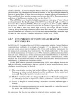
2.2.7 COMPARISON OF FLOW MEASUREMENT
TECHNIQUES
In 1995, the US Geological Survey (USGS) in cooperation with the Federal Highway
Administration outfitted a 61 m length of straight, 137 cm diameter, 0.2 % slope,
concrete storm-sewer pipe in Madison (WI, USA) with multiple instruments for
the purpose of comparing these instruments. The details and results of this study
are briefly summarized in Church et al. (1999). However, additional details of this
field test were obtained as a written communication from D.W. Owens of the USGS
Wisconsin Water Science Center (D.W. Owens, personal communication, 1998).
Because this field test involved three of the previously discussed flow measurement
techniques it is presented as a separate section.
Owens (D.W. Owens, personal communication, 1998) reported that the test site
had the following characteristics that are typical of storm sewer locations where
discharge monitoring may be desired:
(1) The concrete pipe sections had settled different depths creating pipe joints
that acted as minor controls during lower flow conditions. As the water level

increased, the smaller controls were drowned out.
(2) The flow conditions at the site change rapidly because of the small drainage area
(77.7 ha), high amount of impervious surface, and intense summer rainstorms.
(3) Access to the pipe is limited creating a hazardous condition when the pipe is
flowing.
(4) Standard discharge measurements are nearly impossible to collect because of
the access and rapidly changing flow.
He also noted that the site was subject to relatively minor sediment loads.
JWBK117-2.2 JWBK117-Quevauviller October 10, 2006 20:18 Char Count= 0
140 Sewer Flow Measurement
The standard for judging the accuracy of the flows obtained from the various
measurement techniques was a MPB flume (Kilpatrick and Kaehrle, 1986) that had
been rated using 243 dye-dilution flow measurements over a flow range of 0.057 to
2.32 m
3
/s (hereafter referred to as ‘the measurement standard’). The average percent-
age error in the dye dilution discharge calculations was estimated as 4 % with a range
from 1 to 14 % (D.W. Owens, personal communication, 1998). Fifty runoff events
were monitored during a 6-month period and the resulting hydrographs and total
storm runoff volumes obtained with the flow measurement techniques were com-
pared with those obtained with the measurement standard. The flow measurement
techniques evaluated included:
(1) Critical-flow flumes in the form of the theoretical rating for the MPB flume.
(2) Manning’s equation applied at three locations in the study pipe.
(3) AVFMs–Automated Data Systems (ADS), ISCO 4250, and American Sigma
950 Doppler AVFMs and Marsh–McBirney Flow-Tote electromagnetic AVFM.
Data were collected at 1 min intervals for all meters except the ADS meter for which
a 2.5 min interval was used. The meters were placed in series in the pipe.
The comparisons of the measured hydrographs revealed the following (D.W.
Owens, personal communication, 1998):

(1) The hydrographs obtained from the AVFMs are noisier than hydrographs ob-
tained with the measurement standard. Inspection of the data showed that this
resulted from erratic velocity measurements.
(2) The AVFMs had periodic velocity dropouts wherein the velocity measurement
dropped down to a value that was much lower than the previous and following
measurements.
(3) At higher flows (>0.4 m
3
/s), the Doppler AVFMs tended to underestimate the
flow. At lower stages, the Doppler signal tended to work better. These results
are indicative of the range bias for deeper flows that is common for the Doppler
AVFMs.
(4) The electromagnetic AVFM tended to be the closest to the measurement stan-
dard. Furthermore, the electromagnetic velocity measurements displayed less
noise than the Doppler measurements.
(5) The theoretical discharge for the MPB flume closely matched the measurement
standard.
(6) The Manning equation technique produced mixed results based on monitoring
location in the pipe.
Box plots were made of the percentage differences between the results of the
various techniques/equipment and the measurement standard for the total storm
JWBK117-2.2 JWBK117-Quevauviller October 10, 2006 20:18 Char Count= 0
Conclusions and Perspectives 141
runoff volume (Church et al., 1999). Table 2.2.1 was prepared using the same data
used to prepare Figure 7 in Church et al. (1999), which was provided by D.W. Owens
of the USGS Wisconsin Water Science Center. The comparison of the total storm
volumes in Table 2.2.1 yielded the following results:
(1) The electromagnetic AVFM yielded the best overall results with a median error
of 0.4 % and an interquartile range of −9.4 to 4.4 %.
(2) The theoretical rating of theMPB flume also yielded good results with a median

error of +10.8 % and an interquartile range of 2.7 to 17.9 %.
(3) All uncorrected Doppler AVFMs underestimated total storm volumes with me-
dian errors ranging from −6.6 to −28.8 % and mean errors ranging from −10.1
to −30.5 %. Again an indicator of the range bias for deeper flows.
(4) One of the Manning’s equation sites was affected by backwater resulting in a
median error of nearly 100 %. Another Manning’s equation site was affected by
drawdown resulting in 25 % of the storms having underestimates greater than
30 %. The final Manning’s equation site was not affected by either backwater
or drawdown and had a median error of 24.4 % and an interquartile range of
−0.4 to 36.8 %.
It is difficult to derive general results from measurement comparisons at one site,
but Church et al. (1999) raised two important conclusions from this study. The data
clearly indicate the need to calibrate the flow measurement device using measure-
ments obtained with an independent method. Further, although flow measurement
techniques can be adjusted using verification data to minimize bias, the very large
uncertainty in flow measurements exhibited by some of the flow measurement tech-
niques is likely to remain after the adjustments.
2.2.8 CONCLUSIONS AND PERSPECTIVES
Many methods are available for measurement of flow in sewerage systems. Flumes
have been available since the 1930s, and electromagnetic and acoustic methods for
velocitymeasurementhavebeenused sincethe 1970sand1980s, respectively. During
these long periods of use, manufacturers and users have fine-tuned the equipment so
that reliable measurements may be obtained in real-time by telephone line or radio
transmission. If real-time data are desired, users must pay special attention to the
accessibility of the site to power and phone lines or radio transmission to a central
station.
All the flow measurement equipment is capable of yielding accurate discharges for
the appropriate hydraulic conditions (although the range of appropriate conditions
for Manning’s equation is quite limited). Flumes, electromagnetic flow meters and
ADFMs have been found to yield high accuracy (within ±5 %) for a wide range

of flow conditions. However, flumes and electromagnetic meters may be difficult
JWBK117-2.2 JWBK117-Quevauviller October 10, 2006 20:18 Char Count= 0
Table 2.2.1 Summary of storm volume errors in per cent relative to the rated modified Palmer–Bowlus flume for various flow measurement techniques/
equipment applied in a 137 cm diameter in Madison (WI, USA). (Data provided by D.W. Owens, USGS Wisconsin Water Science Center)
Technique/Equipment Mean Median Flow weight (mean) Min. 25th Percentile 75th Percentile Max. No. of storms
Modified Palmer–Bowlus flume
theoretical rating
10.1 10.8 10.2 −20.5 2.7 17.9 23.9 50
Electomagnetic AVFM/Marsh–McBirney
Flow-Tote
−2.2 0.4 0.2 −30.1 −9.4 4.4 24.0 43
Doppler AVFM/American Sigma 950 −30.5 −28.8 −28.0 −58.6 −36.9 −26.0 −8.6 42
Doppler AVFM/ISCO 4250 −10.1 −6.6 −12.4 −27.8 −19.9 −4.4 11.8 33
Doppler AVFM/Automated Data Systems −18.5 −19.0 −22.1 −38.8 −27.7 −14.0 −13.8 29
Manning’s equation/Location 1 −11.6 −0.6 −18.5 −69.8 −30.5 8.0 16.8 50
Manning’s equation/Location 2 18.8 24.4 8.4 −30.1 −0.4 36.8 64.8 48
Manning’s equation/Location 3 99.5 99.3 86.5 34.0 73.0 121.7 155.2 48
142
JWBK117-2.2 JWBK117-Quevauviller October 10, 2006 20:18 Char Count= 0
References 143
to install at some locations. ADFMs are easier to install, but are more costly than
acoustic Doppler area–velocity flow meters. Thus, users must consider site condi-
tions, cost, use of the data, and desired accuracy when selecting the appropriate flow
meter for the project at hand.
Probes for measuring dissolved oxygen concentration, conductivity and temper-
ature in real-time are commonly used in treatment plants and stream systems. Their
use in sewerage systems has been limited due to the possibility of damage by debris
in the confined space of the sewer pipe and the difficulty to keep the probes clean in
the harsh sewer environment. Other probes for measuring nutrients and other chem-
ical constituents in real-time are in development. As these probes are improved,

development of ways to use them in sewerage systems could be very valuable and
is encouraged as a topic of future research and development.
REFERENCES
Alley, W.M. (1977) Guide for Collection, Analysis, and Use of Urban Stormwater Data: A Con-
ference Report, Easton, MD, 28 Novembar–3 December 1976. ASCE.
Anon. (1996) World Water Environ. Eng., April, 36.
Baughen, A.J. and Eadon, A.R. (1983) J. Inst. Water Poll. Cont., 82(1), 77–86.
B¨orzs¨onyi, A. (1982) Advances in Hydrometry, IAHS Publ. No. 134, 19–23.
Church, P.E., Granato, G.E. and Owens, D.W. (1999) Basic Requirements for Collecting,
Documenting, and Reporting Precipitation and Stormwater-Flow Measurements. US Geo-
logical Survey Open-File Report 99–255.
Curling, T., Leafe, M., and Metcalfe, M. (2003) Avoiding the Pitfalls of Dynamic Hydraulic Con-
ditions with Real-Time Data. Available online at />Tideway%20Hydraulic%20Results.pdf.
Day, T.J. (1996) Water Eng. Manage., 143(4), 22–24.
Diskin, M. (1977) J. Irrig. Drain. Div., ASCE, 102(IR3), 383–387.
Doney, B. (1999a) Water Eng. Manage., 146(11), 32–34.
Doney, B. (1999b) Water Eng. Manage., 146(11), 11–12.
Drake, T. (1994) Water Eng. Manage., 141(12), 34.
Hager, W.H. (1989) J. Irrig. Drain., ASCE, 114(3), 520–534.
Hughes, A.W., Longair, I.M., Ashley, R.M. and Kirby, K. (1996) Water Sci. Technol., 33(1), 1–12.
Hunter, R.M., Hunt, W.A., and Cunningham, A.B. (1991) Water Environ. Technol., 3(2), 47–51.
Huth, S. (1998) Water Technol., 21, 78–80.
Johnson, E.H. (1995) Water SA, 21(2), 131–138.
Kilpatrick, F.A. and Kaehrle, W.R. (1986) Trans. Res. Rec., 1073, 1–9.
Lanfear, K.J. and Coll, J.J. (1978) Water Sewage Works, 125(3), 68–69.
Ludwig, R.G. and Parkhurst, J.D. (1974) J. WPCF, 46(12), 2764–2769.
Marsalek, J. (1973) Instrumentation for Field Studies of Urban Runoff. Research Program for the
Abatement of Municipal Pollution Under the Provisions of the Canada-Ontario Agreement on
Great Lakes Water Quality, Ontario Ministry of the Environment, Project 73-3-12.
Melching, C. S. and Yen, B.C. (1986) Slope influence on storm sewer risk. In Stochastic and Risk

Analysis in Hydraulic Engineering, B. C. Yen, ed. Water Resources Publications, Littleton, CO,
pp. 79–89.
JWBK117-2.2 JWBK117-Quevauviller October 10, 2006 20:18 Char Count= 0
144 Sewer Flow Measurement
Metcalf, M.A. and Edelh¨auser, M. (1997) Development of a velocity profiling Doppler flow meter
for use in the wastewater collection and treatment industry. Paper Presented at WEFTEC
’97, available on-line at: />Profiling%20for%20 Wastewater%20Collection%20and%20Treatment.pdf.
Newman, J.D. (1982) Proc. Int. Symp. Hydrometeorology, 15–26.
Palmer, H.K. and Bowlus, F.D. (1936) Adaptation of Venturi flumes to flow measurements in
conduit. Trans. ASCE, 101, 1195–1216.
Parr, A.D., Judkins, J.F., and Jones, T.E. (1981) J. WPCF, 53(1), 113–118.
Soroko, O. (1973) Water and waste flow measurement. TAPPI (Atlanta, GA) Engineering Confer-
ence, Boston, MA, 9 October 1973 (Preprinted Proceedings), pp. 187–203.
Valentin, F. (1981) Water Sci. Technol., 13(8), 81–87.
Waite, A.M., Hornewer, N. and Johnson, G.P. (2002) Monitoring and Analysis of Combined Sewer
Overflows, Riverside and Evanston, Illinois, 1997–99. US Geological Survey Water-Resources
Investigations Report 01-4121.
Watt, I.A. and Jefferies, C. (1996) Water Sci. Technol., 33(1), 127–137.
Wells, E.A. and Gotaas, H.D. (1958) Design of Venturi flumes in circular conduits. Trans. ASCE,
123, 749–771.
Wenzel Jr., H.G. (1975) J. Hydr. Div., ASCE, 101(HY1), 115–133.
Weyand, M. (1996) Water Sci. Technol., 33(1), 257–265.
Wright, J.D. (1991) Water Environ. Technol., 3(9), 78–87.
JWBK117-2.3 JWBK117-Quevauviller October 10, 2006 20:18 Char Count= 0
2.3
Monitoring in Rural Areas
Ann van Griensven and V´eronique Vandenberghe
2.3.1 Introduction
2.3.1.1 Monitoring for the European Union Water Framework Directive
2.3.1.2 Characterisation of Rural Areas and Pollution

2.3.1.3 Joint Use of Modelling and Monitoring
2.3.2 A Case Study
2.3.2.1 The Dender River in Flanders, Belgium
2.3.2.2 The Model Using ESWAT
2.3.2.3 Sensitivity Analysis
2.3.2.4 Uncertainty Analysis
2.3.2.5 Discussion
2.3.3 Automated Monitoring
2.3.3.1 Automated Monitoring Stations
2.3.3.2 The Control of the Station – GSM Communication
2.3.3.3 The Control of the Station – Internet Communication
2.3.3.4 Maintenance and Calibration
2.3.3.5 Discussion
2.3.4 Conclusions and Perspectives
References
Wastewater Quality Monitoring and Treatment Edited by P. Quevauviller, O. Thomas and A. van der Beken
C

2006 John Wiley & Sons, Ltd. ISBN: 0-471-49929-3
JWBK117-2.3 JWBK117-Quevauviller October 10, 2006 20:18 Char Count= 0
146 Monitoring in Rural Areas
2.3.1 INTRODUCTION
2.3.1.1 Monitoring for the European Union Water
Framework Directive
Recently the European Union has approved the European Union Water Framework
Directive (EU WFD). This directive claims that by the end of 2015 a ‘good status
of surface water’ and a ‘good status of groundwater’ should be achieved (European
Union, 2000). To make sure that the new water policy will succeed, a profound
analysis of the actual and future state of the water is necessary. In this context, the
evaluation of emissions into river water will be important.

To that end, the EU WFD provides several guidelines for monitoring the water
bodies, leaving the practical implementation to the local governments. Since urban
pollution has been strongly reduced in many western countries by collection and
treatment of the urban wastewater, the remaining water quality problems require
advanced management and optimisation techniques in an integrated manner. ‘Inte-
grated’ is a term with many interpretations, but also a dangerous term to be used.
Whereas ‘integrated water management’ at first referred to a holistic approach that
linked the sewer–wastewater treatment plant–river systems, it soon became apparent
that goals of good water quality were not reached, causing awareness that some other
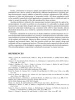
sources of pollution were involved. Indeed, after large investments to reduce urban
pollution, managers were confronted with pollution from rural areas (Figure 2.3.1).
Figure 2.3.1 Sources of pollution in a river basin
JWBK117-2.3 JWBK117-Quevauviller October 10, 2006 20:18 Char Count= 0
Introduction 147
2.3.1.2 Characterisation of Rural Areas and Pollution
Rural areas should not necessarily be considered as pollutant areas. Not-intensive
grazing for instance has beneficial effects on erosion reduction and does not cause
excessive nutrient loads to the receiving systems. In Europe, evolution towards more
intensive practices took place during the past decades and has caused an increase of
nutrient release into theenvironment(Poirot,1999).Underthe Common Agricultural
Policy of the EU, the Gross Value Added (GVA) of the agricultural sector has raised
sharply over the last 25 years. This was mainly due to increased investments giving
in increase in the volume of production (Barthelemy and Vidal, 1999). The measures
have generally led to a reduction of permanent grassland in favour of wheat, maize,
the appearance of oilseed and protein crops and annual crops as fodder. Livestock
production has also followed a trend to intensification, where small extensive hold-
ings are replaced by modern and specialised ones. These ‘nonland-bound’ farms
resulted in a considerable growth in the livestock sector (Boschma et al., 1999).
In particular, pig husbandry constitutes the most intensive type. The intensification
in livestock production and crop culture has led to a high application of nutrients

to agricultural land. Livestock manure is the second most important source in the
EU. The Netherlands and Belgium had the highest input of nitrogen from manure
per hectare coming mostly from pig production (Pau Val and Vidal, 1999). Within
European soils, 115 million hectares suffer from water erosion and 42 million
hectares from wind erosion (Montarella, 1999).
Most agricultural activities are considered to be nonpoint sources. This is not the
case for the large ‘nonland-bound’ farms that are agricultural enterprises where a
large number of animals are kept and raised in confined areas. The feed is generally
brought to the animals, rather than the animals grazing or otherwise seeking feed in
pastures, fields or rangeland. Such activities are treated in a similar manner to other
industrial sources of pollution. Whereas point-source pollution can be measured by
monitoring the discharge and the water quality, diffuse pollution sources are very
difficult to monitor because the sources are distributed along the river.
2.3.1.3 Joint Use of Modelling and Monitoring
An integrated approach with regard to the nonpoint and diffuse pollution creates
new challenges for monitoring and modelling, but it also promotes the interaction
between these two. The water bodies are highly complex systems as they hold many
unknowns and uncertainties due to the incomplete understanding of the processes,
to scaling aspects and to the high variability of the variables in time and space.
Consequently, it is not possible to develop one perfect model or to design an optimal
monitoring network with present information and knowledge. An adaptive approach
is therefore needed: besides linking available data and thereby improving the concep-
tual understanding of the water system, models may indicate errors and inadequacies
in the monitoring network. Conversely, the model is revised and updated as new data
JWBK117-2.3 JWBK117-Quevauviller October 10, 2006 20:18 Char Count= 0
148 Monitoring in Rural Areas
become available. The effects of a pollution load into the river can be evaluated using
models, especially for diffuse pollution, coming from rural areas, because complete
monitoring of diffuse pollution input is impossible. Due to the characteristics of such
a pollution that comes from land use practices, fertiliser and pesticide use, these are

subject to different processes like runoff, leakage to groundwater, uptake by plants,
conversion in the soil and absorption by soil particles. All these can be modelled,
however, for several reasons those model outputs are uncertain (Beck, 1987). Model
outcome uncertainties can become very large due to:
r
input uncertainty;
r
model uncertainty;
r
uncertainty in the estimated model parameter values;
r
mathematical uncertainty.
Therefore, estimating and calculating the diffuse pollution to a river can be subject
to large input uncertainties, so in this chapter we will focus on monitoring with a
view to making the input uncertainties of a model that calculates diffuse pollution
towards a river smaller. To optimally allocate the efforts necessary to reduce those
input uncertainties, it is useful to evaluate the sensitivity of the outputs, the water
quality, to the different inputs needed for calculation of diffuse pollution.
In this study we focus on the diffuse pollution of nitrate in the water due tofertiliser
use. With the use of an efficient Monte Carlo method based on Latin Hypercube
sampling (McKay, 1988), the contribution to the uncertainty by each of the inputs is
calculated. The methodology is applied to the Dender basin in Flanders, Belgium.
The following sections give a description of the river basin for the case study,
the model environment and the applied methodology, which consists of a sensitivity
and uncertainty analysis based on the studies performed by Vandenberghe et al.
(Vandenberghe et al., 2005).
2.3.2 A CASE STUDY
2.3.2.1 The Dender River in Flanders, Belgium
The catchment of the river Dender has a total area of 1384 km
2

and has an average
discharge of 10 m
3
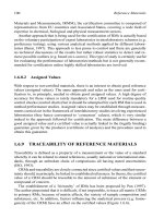
/s at its mouth. Figure 2.3.2 shows how the Dender basin is
situated in Flanders. As about 90 % of the flow results from storm runoff and the
point sources make very little contribution, the flow of the river is very irregular
with high peak discharges during intensive rain events and very low flows during dry
periods (Bervoets et al., 1989). The river Dender is heavily polluted. Part comes from
point-pollution (e.g. industry) but also from diffuse sources of pollution originating
mainly from agricultural activity. Although there is an unmistakable relation between
intensive agricultural activity and the occurrence of high nutrient concentrations in
JWBK117-2.3 JWBK117-Quevauviller October 10, 2006 20:18 Char Count= 0
A Case Study 149
Ijzer
Leie
Boven-
Schelde
Dender
Beneden-
Schelde
Maas
Nete
Demer
Maas
14
15
16
11
13
12

10
8
4
7
5
2
3
6
9
Dijle
Zenne
Brugse
Polders
Gentse
Kanalen
Figure 2.3.2 The River Dender basin in Flanders, Denderbelle (o) and the subbasins
the environment, few precise data are available about the contribution of agricultural
activity to the total nutrient concentrations.
2.3.2.2 The Model Using ESWAT
ESWAT is an extension of SWAT (van Griensven and Bauwens, 2001), the Soil and
Water Assessment Tool developed by the United States Department of Agriculture
(Arnold et al., 1996). ESWAT was developed to allow for an integral modelling
of the water quantity and quality processes in river basins. The diffuse pollution
sources are assessed by considering crop and soil processes. The crop simulations
include growth and growth limitations, uptake of water and nutrients and several
land management practices. The in-stream water quality model is based on QUAL2E
(Brown and Barnwell, 1987). The spatial variability of the terrain strongly affects the
nonpoint source pollution processes. GIS [Geographical Information System(s)] is
used to account for the spatial variability. Based on soil type and land use a number
of Hydrological Response Units (HRUs) can be defined. For each HRU, the ESWAT

model simulates the processes involved in the land phase of the hydrological cycle,
and computes runoff, sediment and chemical loading. Based on the areas of each
HRU, the results are then summed for each subbasin.
Input information for each subbasin is grouped into categories for unique areas
of landcover, soil and management within the subbasins. The main soil classes
are sand, loamsand, silty loam and impervious areas. For landuse, five classes are
important: impervious areas, forests, pasture, corn (maize and corn) and land for
common agricultural use (crop culture, not corn). About 30 % of the landuse is
pasture, while crop farming represents ca. 50 % of the landuse. To build the model,
the total catchment was subdivided into 16 subbasins (Figure 2.3.2).
In terms of the nitrogen cycle, the three major forms in mineral soils are organic
nitrogen associated with humus, mineral forms of nitrogen held by soil colloids and
JWBK117-2.3 JWBK117-Quevauviller October 10, 2006 20:18 Char Count= 0
150 Monitoring in Rural Areas
mineral forms of nitrogen in solution. Nitrogen may be added to the soil by fertiliser,
manure or residue application, fixation by symbiotic or nonsymbiotic bacteria and
rain. Nitrogen is removed from the soil by plant uptake, leaching, volatilisation,
denitrification and erosion.
Nitrate is an anion and is not attracted to or sorbed by soil particles. Because
retention of nitrate by soils is minimal, nitrate is very susceptible to leaching. In
ESWAT the algorithms to calculate nitrate leaching simultaneously solve for loss of
nitrate in surface runoff and lateral flow. Finally nitrate ends in the river.
A previous study for a nitrogen leaching model [implemented in the simulation
model SWIM (soil water infiltration and move)] from arable land in large river
basins (Krysanova and Haberlandt, 2001) showed that the relative importance of
natural and anthropogenic factors affecting nitrogen leaching in the Saale river basin
was as follows: (1) soil; (2) climate; (3) fertilisation rate; and (4) crop rotation.
Reducing the uncertainty on inputs for soil and climate depends on better equipment
to measure the different variables and proper use of sophisticated mathematical
techniques to interpolate for places that are not measured. A lot of studies on that

subject already exist (Sevruk, 1986). Until recently reducing the input uncertainty
relating to fertilisation rate was not studied. In Flanders new legislation concerning
fertilisation application was introduced in the late 1990s. Campaigns to list the
fertiliser use were then started but it is known that a large amount of information is
still wrong or missing. A lot of effort is still needed to complete the information.
The evaluation and quantification of the impacts of land management practices on
nitrogen wash-off to surface water is therefore very important.
In this study we focus on fertilisation rate and time of fertiliser application on the
most important crops for the Dender river basin. For the application of fertiliser for
the different land uses three application dates were assumed; 1 March, 1 April and
1 May. Also, operations such as planting and harvesting dates can be defined. Day
and months were used to specify the planting and harvesting dates. Of course, those
dates depend on the weather, the crop and the farmer, so assumptions had to be made
concerning those dates. The output that was focused upon was the time that nitrate
concentrations in the river Dender at Denderbelle (near the mouth) were higher than
3 mg/l.
The data needed for the model implemented in ESWAT were also very sparse
and conversions had to be made to make the data useful for the model (Smets,
1999). Data on fertiliser and manure use were provided by The Flemish Institute for
Land Use (Vlaamse Landmaatschappij, VLM). They provided data on the nutrient
use and production for each municipality in Flanders. In SWAT, one has to specify
for each subbasin the total amount of fertiliser and the detailed composition of the
fertiliser. Some conversions of the supplied data had to be made so that they could
be used in ESWAT. They consisted of recalculations of the application rates for
each municipality to application rates per subbasin (Smets, 1999). Further, the same
amount of fertiliser on all crops was assumed for this model. This is clearly different
from practice but, at this stage, insufficient details are available to specify this more
realistically.
JWBK117-2.3 JWBK117-Quevauviller October 10, 2006 20:18 Char Count= 0
A Case Study 151

First, a global sensitivity analysis is used to show what the most important factors
are. Then the influence of uncertain data on the river nitrate concentrations time
series is evaluated with an uncertainty analysis. For both the same Monte Carlo
sampled inputs could be used. The sensitivity analysis focuses on the inputs to rank
their importance while the uncertainty analysis assumes uncertain inputs and only
considers and evaluates the outputs.
2.3.2.3 Sensitivity Analysis
The sensitivity analysis (SA) technique used here is based on a multilinear regres-
sion of the inputs on a specific output. A Monte Carlo technique, Latin Hypercube
sampling, makes sure that the total range of inputs is covered. When the number
of samples equals 4/3 times the number of inputs such a sampling is sufficient to
perform a reliable SA (McKay, 1988). For the sampling of the inputs and the analysis
of the outputs, a program was written to couple UNCSAM, the program used for the
SA (Janssen et al., 1992) with the management input files of ESWAT. We used the
standardised regression coefficient (SRC) as an indication of the relative importance
of the different inputs:
SRC
i
=
y/S
y
x
i
/S
x
i
with y/x
i
being the change in output due to a change in an input factor and
S

y
, S
x
i
the standard deviation of, respectively, the output and the input. The input
standard deviation S
x
i
is specified by the user.
The ordering of importance of the input factors based on that statistic is as good
as the associated model coefficient of determination R
2
of the whole multilinear
regression. The closer R
2
is to 1, the better the results.
When the input variables are linearly related, the application of a linear regression
can lead to an accuracy problem, the colinearity problem (Hocking, 1983). The
variance inflation factor (VIF) is defined as:
VIF
i
=
[
C
x
]
ii
=

1 − R

2
i

−1
where [C
x
]
ii
represent the diagonal elements of the covariance matrix relating y
versus x and R
i
2
is the R
2
value that results from regressing y on only x
i
.
For every subbasin the total amount of fertiliser and the time of planting and
harvesting of crops have to be given to the model. A SA can now be performed to
evaluate the influence of those inputs on the model results for nitrate in the river
water. We evaluate the sensitivity of the model on the following result: the time that
nitrate is higher than 3 mg/l. The fractions of mineral HNO
3
, organic N, and NH
3
-N
in the fertilisers are considered to be known and fixed. Hence, we only analyse the
total amount of fertiliser used (Table 2.3.1). As there are a lot of differences in
JWBK117-2.3 JWBK117-Quevauviller October 10, 2006 20:18 Char Count= 0
152 Monitoring in Rural Areas

Table 2.3.1 Composition of the manure as input in SWAT
Chemical Percentage of total fertiliser (100×kg/kg)
HNO
3
28.5
Mineral P 7.5
Organic N 28
Organic P 7.5
Ammonia 28.5
management practices between the different farmers and the time of planting and
harvesting is different from year to year, the plant date and harvest date for the crops
are also considered in the analysis. For a global SA we take the uniform distribution
with standard deviation S
x
i
. The ranges of the uniform distributions are given in
Table 2.3.2. We assumed no correlation. To supply the information on those ranges
a few farmers living in Maarkedal (situated in the Dender basin) were interviewed
about their land management practices.
As the used SA technique is based on linear regression, two measures are calcu-
lated to see whether a linear regression is acceptable.
The first measure is the regression coefficient (RC) which was 0.845 for the whole
multilinear regression. Because this value is close to 1 and the F-statistic showed that
the regression is significant, a linear regression is adequate. The value of0.845means
that there is a fraction of the output variance, 15.5 %, that is left unaccounted for.
The second measure is the VIF. The largest VIF for this analysis was 1.35. A VIF
smaller than 5 means that the correlation between the inputs is small enough to allow
application of a linear regression (Janssen et al., 1992). The SRC is significant on
the 10 % level for eight parameters. In Table 2.3.3 the parameters are ranked.
For river nitrate concentrations the amount of fertiliser used in the subbasins that

are laying upstream are especially important. This SA also shows that it is more
important to focus on the amount of fertiliser than on the management practices.
2.3.2.4 Uncertainty Analysis
The Flemish Institute for Land Use provided input data for the model. Due to unreg-
istered manure and fertiliser use, it is very likely that those data are underestimated.
The amount of fertiliser was the same for all crops, which is unrealistic and it is very
Table 2.3.2 Ranges for global sensitivity analysis of management practice
inputs for nitrogen
Input Uncertainty
Plant date for the crops ±1 month
Harvest date of the crops ±1 month
Amount of fertiliser applied per subbasin and per crop (kg/ha) ±25 %
JWBK117-2.3 JWBK117-Quevauviller October 10, 2006 20:18 Char Count= 0
A Case Study 153
Table 2.3.3 The eight most important inputs, their SRC and their sensitivity ranking
Input SRC Rank
Amount of fertilisation on pasture in subbasin 16 −0.303 1
Amount of fertilisation on farming land in subbasin 4 0.226 2
Growth date of pasture −0.183 3
Plant date on farming land 0.171 4
Amount of fertilisation on corn in subbasin 5 −0.169 5
Amount of fertilisation on corn in subbasin 15 −0.165 6
Amount of fertilisation on pasture in subbasin 12 0.159 7
Amount of fertilisation on corn in subbasin 11 0.155 8
likely that thecompositionof the fertiliser used isnotalways thesameas wasassumed
here. The uncertainty of the latter two generalisations is included in the uncertainty
in the amount of fertiliser used on the crops. Such an uncertainty is propagated
through the model and gives a final uncertainty on the model results of the water
quality near the mouth of the river. An uncertainty analysis in which all of the un-
certain sources are varied at the same time is performed to see the effects of the

uncertainty of the inputs. For this analysis we calculate the uncertainty bands, i.e.
the 5% and 95 % percentiles for the results of the time series obtained after sampling
the inputs as also done in the SA.
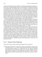
Figure 2.3.3 illustrates the contribution of an uncertainty of up to 25 % to the
amount of fertiliser applied on the crops and an uncertainty of 1 month for the
plant and harvest dates. The 95 % bound shows much higher peaks than the mean
concentration–time series. This means that some peak values of nitrate in the river
water at Denderbelle may not be predicted properly due to an underestimation of the
amount of fertiliser used. Those peaks (e.g. days 156 and 260) are above levels of
nitrate concentrations for basic water quality.
Only a few measurements were available for the calibration of the model using a
multi-objective automated calibration method (van Griensven and Bauwens, 2003).
As can be seen, some of the measuring points are available at time instants where
the uncertainty on the inputs is not propagated. Fortunately, the model calibration
was successful. The data around day 340 are within the uncertainty bound, but the
ones on day 240 are clearly not predicted well.
The inputs we considered uncertain in this study are only a fraction of all the
inputs that cause uncertainty, but it is shown that the inputs related to fertiliser use
already give a large uncertainty in certain periods ofthe year (95 % percentile bounds
differs up to ±50 % from the average nitrate predictions). Those are periods with
rainfall and high flows. Knowing that there are more sources of uncertainty related
to diffuse pollution, the input uncertainty is expected to be even higher. Therefore it
is clear that care has to be taken during the gathering of data needed to run a dynamic
process-based model for the prediction of effects of diffuse pollution.
This uncertainty analysis shows also some important results for future measure-
ment campaigns. This study shows that we could obtain a better calibration for the
JWBK117-2.3 JWBK117-Quevauviller October 10, 2006 20:18 Char Count= 0
154 Monitoring in Rural Areas
0
2

4
6
8
10
12
14
16
18
1 26 52 78 104 130 156 182 208 234 260 286 312 337 363
time (days)
Nitrate (mg/l)
mean
95% percentile
5% percentile
measuring points
5
(a)
(b)
4.5
3.5
2.5
1.5
0.5
0
3
2
1
4
3653393132872612352091831571311057953271
time (days)

rainfall (mm)
0
10
20
30
40
50
60
70
80
90
100
flow (m
3
/s)
rainfall
flow
Figure 2.3.3 The simulated flow rate and rainfall measurements (a) and simulations of nitrate
with the 5 % and 95 % confidence intervals (b) in the Dender river at Denderbelle for the year 1994
diffuse pollution part of the model with data that were taken during periods with
rainfall and high flows, because the model output nitrate is more sensitive towards
inputs of diffuse pollution in those periods. If you want to focus on calibrating the
in-stream behaviour and point pollution then measurements during dry periods are
needed as the model is then not sensitive towards input of diffuse pollution.
2.3.2.5 Discussion
The model output for nitrate in river water is sensitive towards eight inputs related to
fertiliser use. These are the start date of the growth of pasture, plant date on farming
land, the amount of fertiliser applied on pasture in subbasins 16 and 12, on farming
land in subbasins 4 and on corn in subbasins 5, 11 and 15. The dates of planting and
harvesting the crops appear not to be important. To reduce the output uncertainty it

is best to focus on data about amounts of fertiliser applied on crops.
In the uncertainty analysis, the effects of uncertain input of fertiliser use and land
management on nitrate concentrations in the river are shown. In certain periods of
JWBK117-2.3 JWBK117-Quevauviller October 10, 2006 20:18 Char Count= 0
Automated Monitoring 155
the year the uncertainty bounds are very wide. Because there are more sources of
uncertainty, not considered in this study, it becomes clear that it is very important
to gather accurate data to run a dynamic process-based model for the prediction of
effects of diffuse pollution.
The uncertainty analysis is also of great use for experimental design. Measure-
ments during dry periods can be used to better calibrate the model for point source
pollution because the inputs of diffuse pollution are not important then. On the other
hand, periods with rainfall and high flows are needed for the calibration of the model
with diffuse pollution because the model output for nitrate is then very sensitive
towards the inputs related to farmer’s practices.
More detailed studies are needed to see the exact contribution of the input un-
certainties to the output uncertainty. We can already conclude on the basis of this
study that uncertainty analysis is an essential part of diffuse pollution modelling to
evaluate and draw conclusions from model predictions.
2.3.3 AUTOMATED MONITORING
The Dender model clearly illustrates the high variability in water quantity and quality
in rural areas. It is therefore hard to plan monitoring for certain preferred conditions
(dry period versus rain event). In practice, it may not be feasible to catch these short
events through manual sampling.
2.3.3.1 Automated Monitoring Stations
Automated Measuring Stations (AMSs) can be very helpful to capture specific dy-
namics through continuous monitoring or through controlled inducing of samplers
by using the signals for the river level, for precipitation or for sediment concentra-
tions (van Griensven et al., 2002; Vandenberghe et al., 2004). Figure 2.3.4 shows
one of three AMSs that were placed on the Dender river in Belgium and that are

connected through SMS (Short Message Service) communication or the internet
to a central computer/database. In the station, the river water is pumped through a
Figure 2.3.4 AMS on the Dender river
JWBK117-2.3 JWBK117-Quevauviller October 10, 2006 20:18 Char Count= 0
156 Monitoring in Rural Areas
Table 2.3.4 The sensors in the station
Variable Method Range Compensation Frequency
pH Combined glass electrode 0–14 Temperature Continuous
Dissolved oxygen
(% sat)
Galvanic electrode 0–200 Temperature Continuous
Redox potential
(ORP) (mV)
Pt + Ag/AgCl electrode −1000–1000 Temperature Continuous
Turbidity (NTU) Photo-electric meter 0–200 Temperature Continuous
Conductivity
(μS/cm)
Pt electrode 0–9999 Temperature Continuous
Ammonium-N
(ppm)
Ion-selective electrode 0.1–14000 Not automatic Every 15 min
Nitrate-N (ppm) Ion-selective electrode 0.1–14000 Not automatic Every 15 min
Solar radiation
(W/m
2
)
Pyranometer 0–4000 No Continuous
Precipitation Tipping bucket No 0.254 mm
Water level Pressure electrode No Continuous
Temperature (

◦
C) Pt100 −10–120 — Continuous
hydraulic loop. At the entrance of the loop, the turbidity is measured and a bypass to
a sampling system is available. After filtration (100 μm), temperature, conductivity,
pH, dissolved oxygen and redox potential are measured in the loop. Ammonia and
nitrate can be measured with ion-selective electrodes in off-line reservoirs to which
buffer solutions are added. Solar radiation, precipitation and water level are also
measured in situ. Table 2.3.4 lists the characteristics of the sensors.
2.3.3.2 The Control of the Station – GSM Communication
In the case where only GSM (Global System of Mobile Communication) is avail-
able, SMS messages – containing the data and alarms – are automatically sent to a
remote central computer (Figure 2.3.5). Daily, the data of the central computer are
automatically backed up and imported into a relational database.
Remote control (through SMS) is limited to:
r
the transmission of the latest data set (data and alarms);
r
the start-up of a predefined sampling program.
2.3.3.3 The Control of the Station – Internet Communication
When an internet connection is available, the LabView interface enables remote
interaction with the station. The interface optimises the follow up of the station by a
front panel that visualises the hydraulic loop and displays the actual measurements
JWBK117-2.3 JWBK117-Quevauviller October 10, 2006 20:18 Char Count= 0
Automated Monitoring 157
ADSL, cable modem
of direct connection
GSM-SMS
Internet
INTERNET
• direct control of PC is

possible
• sending measurements to
central computer
• sending alarms through
E-mail
GSM
• limited control possible (ex.steering of sampler)
• sending measurements to central computer
• sending alarms to GSM
Figure 2.3.5 Communication of the automated and transportable on-line monitory system
(ATOMS) and the LabView ( National Instruments Software)
and alarms (Figure 2.3.5). A plot with the recent evolution of the measured water
quality variables can also be displayed. The central database is hereby continuously
updated.
Remote control of the operation of the system is facilitated by:
r
the visualisation of alarms on the panels, in case of malfunctioning of the sensors
(signal out of range), low flow or low pressure in the loop or low air temperature
in the cabin;
r
the sending of GSM messages and/or emails to selected team members;
r
the on-line adaptation of control parameters (e.g. logging interval);
r
the on-line control of the sampler;
r
the availability of a WebCam.
2.3.3.4 Maintenance and Calibration
Automated maintenance consists of the rinsing of the filter and the electrodes by
injection of air under pressure (after every logging). The station requires a weekly

maintenance visit by two team members to clean the filters and the sensors and, if
necessary, calibrate the sensors. A LabView program guides the calibration process.
After the calibration, a log file with the new calibration parameters is logged and the
measuring mode is started again.
2.3.3.5 Discussion
AMSs are useful tools for monitoring in rural areas under the conditions that the
monitoring system coincides with good maintenance and quality control. In practice,