JWBK117-1.6 JWBK117-Quevauviller October 10, 2006 20:14 Char Count= 0
100 Reference Materials
Materials and Measurements, IRMM), the certification committee is composed of
representatives from EU countries and Associated States, covering a wide field of
expertise in chemical, biological and physical measurement sectors.
Another approach that is being used for the certification of RMs is actually based
on the voluntary participation of expert laboratories in interlaboratory schemes (e.g.
proficiency testing), using various analytical methods applied by different labora-
tories (Ihnat, 1997). This approach is less prone to control and there are generally
no technical discussions of the results but rather robust statistics to detect and re-
move possible outliers (e.g. based on z-scores). This type of study is certainly useful
for evaluating the performance of laboratories/methods but is not generally recom-
mended for certification unless highly skilled laboratories are involved.
1.6.8.2 Assigned Values
With respect to not-certified materials, there is an interest to obtain good reference
values (assigned values). The same approach and rules as the ones used for certi-
fication to, in principle, needed to obtain good assigned values. A high degree of
accuracy for these values is rarely mandatory for a LRM used for routine quality
control checks (control charts) but it should be attempted for each RM that is used in
method performance studies. Assigned values may be established through measure-
ments carried out in the framework of interlaboratory studies involving experienced
laboratories (they hence correspond to ‘consensus’ values), which is very similar
indeed to the approach followed for certification. The main difference between a
good assigned value and a certified value is actually linked to the (legally binding)
guarantee given by the producer (certificate of analysis) and the procedure used to
obtain this guarantee.
1.6.9 TRACEABILITY OF REFERENCE MATERIALS
Traceability is defined as a property of a measurement or the value of a standard
whereby it can be related to stated references, usually national or international stan-
dards, through an unbroken chain of comparisons all having stated uncertainties
(ISO, 1993).

CRMs and traceability arecloselyconnectedsincecertified values andtheir uncer-
tainty should, in principle, be linked to established references. In theory, the certified
value of a CRM should be traceable to the amount of substance of the element or
compound of concern.
The establishment of a ‘hierarchy’ of RMs has been proposed by Pan (1997).
The author pinpointed that it is difficult, if not impossible, to trace all matrix CRMs
to primary RMs, because of matrix effects, the variety of sample composition and
substances, etc. In addition, factors influencing the analytical process (e.g. homo-
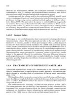
geneity of the CRM) have an effect on the certified values (Figure 1.6.6).
JWBK117-1.6 JWBK117-Quevauviller October 10, 2006 20:14 Char Count= 0
Traceability of Reference Materials 101
True value
Global and local
comparability
CRM, PT schemes
accreditation
Internal comparability
International Quality Control, LRM
Appropriate calibration
Measurement of samples
Figure 1.6.6 Traceability hierarchy shows how to achieve results close to the true values
The classification proposed provided the main criteria for establishing a hierarchy
in the traceability chain for CRMs:
r
metrological quality of methods used for certifying values of the CRM;
r
homogeneity and stability;
r
calculation of uncertainty;
r

metrological competence and recognition of the producer at the national and/or
international level;
r
demonstration of traceability.
Numerous chemical measurements are carried out, for which RMs cannot readily
be prepared owing to their instability (Richter and Dube, 1997). In other cases, RMs
may beavailable but theirmatrices aresignificantly differentfrom that ofthe analysed
sample, and the reference used to demonstrate the traceability of the results is then
questionable. Some CRMs are directly traceable to SI units and open the possibility
of traceability of measurements to these units, e.g. high purity substances, stable
isotope calibrants for IDMS, playing the role of primary RMs (Richter and Dube,
1997).
The user of a CRM and of certified values should be informed about all the
aspects of traceability that have directed the preparation and certification of the RM,
the technical explanations on the rejection of outlying results, the sources of error,
the procedures of recovery evaluation (based on a spiking procedure or the analysis
of another CRM), the available documentation on the CRMs used to validate the
certification methods, etc.
JWBK117-1.6 JWBK117-Quevauviller October 10, 2006 20:14 Char Count= 0
102 Reference Materials
1.6.10 EVALUATION OF ANALYTICAL RESULTS USING
A MATRIX CERTIFIED REFERENCE MATERIAL
This section will examine how an analytical result may be evaluated in comparison
with the certified value of a matrix CRM. The approach described is adapted from
the procedure proposed by Walker and Lumley (1999). The general use of RMs in a
validation process of a method is described in detail by them (Walker and Lumley,
1999). The use of a matrix CRM will be based on the evaluation of an analytical
result (x) as compared with a certified value (μ) of the CRM. The error on the
analytical result () is calculated using the formula:  = x − μ.
Considering the random errors of the method, the value of  will likely not be

equal to zero, even if the result is not affected by any systematic error. The greater
the random errors (i.e. the poorer the precision), the greater the value of  and
hence the more difficult to detect the occurrence of a systematic error. The precision
is, therefore, a critical parameter that should not be underestimated when evaluating
the trueness of a method. Walker and Lumley (1999) distinguish the laboratory
internal standard deviation, s
i
, characterized by the measurement repeatability of
which the estimate should be calculated on the basis of at least seven repetitions of
CRM analyses, and the between-laboratory standard deviation, s
e
, which is more
difficult to estimate. The authors propose several approaches to calculate this latter
parameter:
(1) The reproducibility, s
R
, may be estimated by replicate analyses (at least 7,
preferably up to 20) carried out over a given period of time (if possible over 3
months).
(2) The between-laboratory standard deviation, s
e
, may also be estimated in the
framework of any method validation interlaboratory study in which the labora-
tory will know the repeatability values, s
r
, and the reproducibility values, s
R
,of
the method according to the document summarizing the results of the study. The
value of s

e
will hence be equal to
√
(s
2
R
− s
2
r
).
(3) When the CRM has been characterized in the framework of an interlaboratory
study, information on the between-laboratory standard deviation are generally
given in the certification report of the material. If the method to be tested is
similar to one of those used for the certification of the RM, the value of s
e
given
in the report may be used.
(4) Predicted values found in the literature may also enable the estimate of s
e
. This
type of information is available in the agro-food sector but few values compar-
atively exist in the sector of water analysis.
(5) In the absence of any information, an estimate of s
e
may be obtained from the
value of s
i
according to the formula: s
e
≈ 2s

i
.
JWBK117-1.6 JWBK117-Quevauviller October 10, 2006 20:14 Char Count= 0
Evaluation of AnalyticalResults Usinga Matrix CertifiedReferenceMaterial 103
The precision σ of an analytical result of a matrix CRM will be calculated by
combination of two components:
σ =
√

s
2
e
+ s
2
i
n

where n is the number of replicates of CRM analyses. In general, the value s
i
is
smaller than the value of s
e
(typically by a factor of 2 as indicated above). The fact
that n is at least equal to 7 means that s
e
will represent the main contribution of σ .
At first sight, it could appear sufficient to base the estimate of the precision σ
of a method used by an individual laboratory on the sole value of s
i
. However, s

i
reflects the random dispersion of results of a series around their mean, which is
itself randomly distributed around the CRM certified value with a dispersion that is
characterized by the value s
e
. Therefore, the combination of s
i
and s
e
(as indicated
above) is used to describe the overall dispersion of the results around the certified
value, which is taken as the true value (Walker et Lumley, 1999).
The parameter s
e
measures the sources of random errors that cannot be evaluated
by replicate analyses in a single laboratory, but however contribute to the result
dispersion around the certified value (true or assigned value). An example of random
error is the possible variation of the final volume of a sample extract before its
introduction in a measurement instrument, without taking care of the variations
of ambient temperature. Such volume variations would not be significant for the
estimate of the repeatability and would therefore not be considered in the calculation
of s
i
. However, the same measurements carried out by different laboratories (or by
a single laboratory over a given period of time) would be suject to random errors
due to variations of the ambient temperature. The effects of such variations would
be included in the term s
e
.
It is also useful to remember that when a laboratory analyses a matrix CRM, it

actually takes an effective part in an ‘interlaboratory study’ (if the certified values
have indeed been measured on the basis of such study). Under these circumstances,
it is clearly appropriate that the component s
e
of the precision be considered when a
laboratory compares its results to CRM values. This is analogous to the comparison
of laboratory results in the framework of proficiency testing schemes using z scores
[see additional information in Quevauviller (2001)].
If the information on the value s
i
is available (e.g. the repeatabilty value s
r
of
the method as validated through an interlaboratory study), a χ
2
test may then be
carried out that will establish whether s
i
(measured by the laboratory) is acceptable,
i.e. whether the laboratory performs its method with a sufficient precision. However,
even if s
i
is significantly greater than s
r
, if the measured value s
2
i
/
√
n is small in

comparison to s
2
e
, there will be little or no benefit to repeat a series of measure-
ments of a CRM with the aim to obtain a smaller value of s
i
(Walker and Lumley,
1999).
JWBK117-1.6 JWBK117-Quevauviller October 10, 2006 20:14 Char Count= 0
104 Reference Materials
The estimate of the possible occurrence of systematic errors will be based on a
statistical test aiming to evaluate whether the value  is significantly different from
zero. If it is not the case, it is possible to conclude that no systematic error has been
demonstrated. A test that is currently used is based on bracketing the value  in
an interval with limits of ±2σ in which it is estimated that no systematic error has
occurred: −2σ<<2σ .
The affirmation that no systematic error has occurred has to be considered with
some care. It is indeed possible that errors are left undetected, e.g. in the case of
positive and negative errors, which compensate each other. As previously mentioned,
the choice of the ±2σ interval means that the confidence level of this conclusion is
about 95 %. The adoption of limits ±3σ would permit to obtain a confidence level
of 99.7 %. This is equivalent to the calculation of z scores used in proficiency testing
schemes [as a reminder, z = (x − X)/σ, the value of σ being based, in this case, on
the standard deviation resulting from the test].
It is important that the value of σ be a reliable estimate of the measurement pre-
cision. Among the five above-described approaches, procedure (1) implies that at
least seven replicate analyses be carried out (which is generally considered suffi-
cient). However, if the method has been previously studied (enabling to be obtained
a good estimate of the standard deviation of the measurement for the considered
matrix) the number of CRM analyses may be less than seven, although the minimum

is to duplicate the analysis. A single analysis may be envisaged where the laboratory
is confident in its statistical control. The value of n used for the calculation of σ
should obviously reflect the number of replicate analyses effectively carried out on
the CRM.
Walker and Lumley (1999) give an example of application related to water analy-
sis: A water CRM containing certified concentrations of herbicides (LCG 1004)
is analysed six times. The certified value of simazine is equal to (26.7 ± 2.0) μg
kg
−1
, and the values obtained by the laboratory are, respectively, 29.4, 24.9, 26.4,
25.7, 22.0 and 23.5, corresponding to a mean concentration of 25.3 μgkg
−1
and
a standard deviation of 2.5 μgkg
−1
. The adopted value for s
e
is 5.2 μgkg
−1
,
based on the measurement of the measurement reproducibility. The value of σ
is, therefore, equal to: σ =
√
[(5.2)
2
+ (2.5)
2
/6] = 5.3 μgkg
−1
.

The calculated value of  obtained is: 25.3 −26.7 =−1.4 μgkg
−1
.
It is hence verified that this value responds to the conditions of acceptability
of the method, i.e. −10.6 < 1.4 < 10.6.
Let us note once more that the validity of the above-described test depends upon
the validity of the adopted values for s
i
and s
e
. If these values are erroneous, the
value of σ will be also erroneous, and the test will lead to wrong conclusions.
In some cases, it appears necessary to take into account the uncertainty of the
certified value of the CRM (if this uncertainty is significantly different from σ) and
JWBK117-1.6 JWBK117-Quevauviller October 10, 2006 20:14 Char Count= 0
Reference Material Producers 105
to add a term corresponding to an enlarged uncertainty. Further details can be found
in the literature (Walker and Lumley, 1999; ISO, 2000a,b).
The error may be expressed in two different ways in the framework of a method
validation:
(1) As an absolute value |x – x
o
| where a positive error indicates a higher value.
Or (more often in the case of method validation):
(2) As arecovery factor, i.e. a fraction ora percentage, x/x
o
or 100x/x
o
, where x is the
measured value and x

o
the certified value. This type of approach is particularly
useful when several tests or materials are subject to similar and proportional
errors.
1.6.11 REFERENCE MATERIAL PRODUCERS
More than 150 reference material producers exist worldwide, but few of them are
dedicated to water analysis. Information on the available materials can be obtained
from the searchable VIRM database (), a member-led nonprofit
organization founded within the 6th EC Framework programme, the COMAR data
base, which is jointly operated by the BAM (Berlin, Germany), the LGC (London,
UK) and the LNE (Paris, France). It should be noted that the mandatory criteria
with respect to production quality (in particular accreditation) are not always ful-
filled and that, therefore, it is presently difficult to evaluate the quality of all the
materials that are available on the market. Among the major producers, two major
organizations cover a large range of CRMs (including water CRMs) and ensure a
continuity of the stocks: these are, on the one hand, the BCR in Europe (Institute
for Reference Materials and Measurements, European Commission Joint Research
Centre, Geel, Belgium) and, on the other hand, the NIST in the USA (National Insti-
tute for Standards and Technology, Gaithersburg, MD, USA). These two organiza-
tions deliver catalogues that can be obtained free of charge and provide information
on the Internet ( for IRMM; />for NIST). Other notable producers for water CRMs are the National Research
Council of Canada (Ottawa, Canada), the National Research Centre on CRMs
in Pekin (China) and the National Institute for Environmental Sciences in Osaka
(Japan). Other organizations produce water (C)RMs for the purpose of proficiency
testing schemes in support of laboratory accreditation, e.g. the National Water Re-
search Institute (USA) and the Dutch Ministry of Public and Water Works (The
Netherlands).
Various CRMs for the quality control of water analysis, covering different types of
matrices (freshwater, estuarine water, seawater, groundwater) are described in Vol-
ume 3 ofthe WaterQuality MeasurementsSeries (Quevauviller, 2002). InTable 1.6.4,

the currently available CRMs related to wastewater are summarized, excluding the
above-discussed BCR materials.
JWBK117-1.6 JWBK117-Quevauviller October 10, 2006 20:14 Char Count= 0
106 Reference Materials
Table 1.6.4 Certified and indicative analyte concentrations of currently available
wastewater-related CRMs in Europe
RM code Provider and
and matrix Analyte Value contact details
CRM002-100
Activated
charcoal
water filter
Aluminium 1800 mg kg
−1
(Noncertified) RT Corporation
http://www.
rt-corp.com
Antimony 2 mg kg
−1
(Noncertified)
Arsenic 30 mg kg
−1
(Noncertified)
Barium 80 mg kg
−1
(Noncertified)
Boron 80 mg kg
−1
(Noncertified)
Cadmium 1 mg kg

−1
(Noncertified)
Calcium 980 mg kg
−1
(Noncertified)
Chromium 36300 mg kg
−1
(Certified)
Cobalt 10 mg kg
−1
(Noncertified)
Copper 96900 mg kg
−1
(Certified)
Iron 1150 mg kg
−1
(Noncertified)
Lead 5 mg kg
−1
(Noncertified)
Magnesium 190 mg kg
−1
(Noncertified)
Manganese 8 mg kg
−1
(Noncertified)
Mercury 5 mg kg
−1
(Noncertified)
Nickel 30 mg kg

−1
(Noncertified)
Potassium 490 mg kg
−1
(Noncertified)
Selenium 4 mg kg
−1
(Noncertified)
Silver 18.3 mg kg
−1
(Certified)
Sodium 480 mg kg
−1
(Noncertified)
Strontium 110 mg kg
−1
(Noncertified)
Thallium 20 mg kg
−1
(Noncertified)
Tin 120 mg kg
−1
(Noncertified)
Titanium 210 mg kg
−1
(Noncertified)
Vanadium 40 mg kg
−1
(Noncertified)
RM2 and

RM2e
Wastewater
Biological oxygen
demand
13–216 mg O
2
L
−1
(Noncertified) Association
G´en´erale des
Laboratoires de
l’Environnement

Chloride 95–600 mg L
−1
(Noncertified)
Chemical oxygen
demand
50–1000 mg O
2
L
−1
(Noncertified)
Conductivity 1150–1530 μScm
−1
(Noncertified)
Fluorine 0.3–4.5 mg L
−1
(Noncertified)
Potassium 14–35 mg L

−1
(Noncertified)
Suspended solids 11–250 mg L
−1
(Noncertified)
Sodium 71–163 mg L
−1
(Noncertified)
Ammonia 0.6–56 mg N L
−1
(Noncertified)
Nitrite <0.05–3.5 mg N L
−1
(Noncertified)
Nitrate <0.2–150 mg N L
−1
(Noncertified)
Total phosphorous 2–11 mg P L
−1
(Noncertified)
pH 7.1–8 (Noncertified)
Phosphate 1.5–5.75 mg P L
−1
(Noncertified)
Sulfate 112–142 mg L
−1
(Noncertified)
Total Kjeldahl nitrogen 6–104 mg N L
−1
(Noncertified)

Total organic carbon 60 mg C L
−1
(Noncertified)
JWBK117-1.6 JWBK117-Quevauviller October 10, 2006 20:14 Char Count= 0
Table 1.6.4 (Continued )
RM code Provider and
and matrix Analyte Value contact details
RM3B
Wastewater
Aluminium 85–2000 μgL
−1
(Noncertified) Association
G´en´erale des
Laboratoires de
l’Environnement

Arsenic 1.5–80 μgL
−1
(Noncertified)
Boron 300–2850 μgL
−1
(Noncertified)
Barium 65–425 μgL
−1
(Noncertified)
Beryllium 10 μgL
−1
(Noncertified)
Cadmium 1–490 μgL
−1

(Noncertified)
Cobalt 140 μgL
−1
(Noncertified)
Chromium 4.5–3500 μgL
−1
(Noncertified)
Copper 40–12000 μgL
−1
(Noncertified)
Iron 100–2500 μgL
−1
(Noncertified)
Mercury 0.3–50 μgL
−1
(Noncertified)
Manganese 180–1100 μgL
−1
(Noncertified)
Molybdenum 480 μgL
−1
(Noncertified)
Nickel 35–7000 μgL
−1
(Noncertified)
Lead 10–3000 μgL
−1
(Noncertified)
Selenium <5–85 μgL
−1

(Noncertified)
Tin 500 μgL
−1
(Noncertified)
Titanium <10–200 μgL
−1
(Noncertified)
Zinc 10–9000 μgL
−1
(Noncertified)
RM4B and 60
Wastewater
1,2-Dichloroethane 1–130 μgL
−1
(Noncertified) Association
G´en´erale des
Laboratoires de
l’Environnement

Aldrin 0.003–0.10 μgL
−1
(Noncertified)
Anthracene 0.02–0.15 μgL
−1
(Noncertified)
Atrazine 0.1–0.6 μgL
−1
(Noncertified)
Benzene 5–35 μgL
−1

(Noncertified)
Benzo(a)anthracene 0.02–0.15 μgL
−1
(Noncertified)
Benzo(a)pyrene 0.02–0.15 μgL
−1
(Noncertified)
Benzo(b)fluoranthene 0.02–0.25 μgL
−1
(Noncertified)
Benzo(g,h,i)perylene 0.02–0.20 μgL
−1
(Noncertified)
Benzo(k)fluoranthene 0.02–0.15 μgL
−1
(Noncertified)
Bromodichloromethane 0.95–3 μgL
−1
(Noncertified)
Bromoform 1–5.5 μgL
−1
(Noncertified)
Carbon tetrachloride 0.1–1.5 μgL
−1
(Noncertified)
Chloroform 1–7.5 μgL
−1
(Noncertified)
Chlortoluron 0.1–0.65 μgL
−1

(Noncertified)
Deisopropylatrazine 0.1–0.4 μgL
−1
(Noncertified)
Desethylatrazine 0.05–0.9 μgL
−1
(Noncertified)
Diazinon 0.4 μgL
−1
(Noncertified)
Dibenzo(a,h)anthracene 0.02–0.40 μgL
−1
(Noncertified)
Dibromochloromethane 1–5.5 μgL
−1
(Noncertified)
Dieldrin 0.01–0.20 μgL
−1
(Noncertified)
Diuron 0.1–0.9 μgL
−1
(Noncertified)
Ethion 0.2 μgL
−1
(Noncertified)
Fluoranthene 0.02–0.25 μgL
−1
(Noncertified)
Heptachlor 0.009–0.060 μgL
−1

(Noncertified)
Heptachlor epoxide 0.01–0.090 μgL
−1
(Noncertified)
Indeno(1,2,3-cd)pyrene 0.02–0.10 μgL
−1
(Noncertified)
Isoproturon 0.08–0.8 μgL
−1
(Noncertified)
Lindane 0.01–0.26 μgL
−1
(Noncertified)
Linuron 0.1–0.65 μgL
−1
(Noncertified)
Methyl(2)fluoranthene 0.02–0.085 μgL
−1
(Noncertified)
(Continued )
107
JWBK117-1.6 JWBK117-Quevauviller October 10, 2006 20:14 Char Count= 0
Table 1.6.4 Certified and indicative analyte concentrations of currently available
wastewater-related CRMs in Europe (Continued )
RM code Provider and
and matrix Analyte Value contact details
Methyl(2)naphthalene 0.02–0.080 μgL
−1
(Noncertified)
PCB 101 0.005–0.75 μgL

−1
(Noncertified)
PCB 118 0.005–0.45 μgL
−1
(Noncertified)
PCB 138 0.005–0.85 μgL
−1
(Noncertified)
PCB 153 0.005–0.90 μgL
−1
(Noncertified)
PCB 180 0.005–0.70 μgL
−1
(Noncertified)
PCB 28 0.005–0.035 μgL
−1
(Noncertified)
PCB 52 0.005–0.35 μgL
−1
(Noncertified)
Propazine 0.1–0.4 μgL
−1
(Noncertified)
Simazine 0.1–0.7 μgL
−1
(Noncertified)
Terbutylatrazine 0.1–0.7 μgL
−1
(Noncertified)
Tetrachloroethylene 0.2–0.80 μgL

−1
(Noncertified)
Toluene 5–40 μgL
−1
(Noncertified)
Total xylene 5–40 μgL
−1
(Noncertified)
Trichloroethylene 1–5 μgL
−1
(Noncertified)
RM51 Arsenic <100–450μgkg
−1
dry wt (Noncertified) Association
G´en´erale des
Laboratoires de
l’Environnement

Wastewater Cadmium <100 μgkg
−1
dry wt (Noncertified)
Chromium <200–5800 μgkg
−1
dry wt (Noncertified)
Copper <300–1500 μgkg
−1
dry wt (Noncertified)
Mercury <10–25 μgkg
−1
dry wt (Noncertified)

Nickel <200 μgkg
−1
dry wt (Noncertified)
Lead 1.1–13 μgkg
−1
dry wt (Noncertified)
Selenium <200–450μgkg
−1
dry wt (Noncertified)
Soluble fraction 2.5–40 % dry wt (Noncertified)
Zinc 850–7000 μgkg
−1
dry wt (Noncertified)
RM5B
Wastewater
Anionic surfactants
index
500–20000 μg SDS L
−1
(Noncertified) Association
G´en´erale des
Laboratoires de
l’Environnement

Phenol index 100–20000 μgC
6
H
5
OH L
−1

(Noncertified)
Total cyanide index 250 μgCNL
−1
(Noncertified)
Total hydrocarbons
index
200–13000 μgL
−1
(Noncertified)
VKI-HL1 Aluminium 2.07 μgL
−1
(Certified) Eurofins A/S
www.eurofins.dk/
referencematerials
Wastewater Iron 3.03 μgL
−1
(Certified)
Manganese 1.98 μgL
−1
(Certified)
Molybdenum 9.96 μgL
−1
(Certified)
Lead 10.02 μgL
−1
(Certified)
Tin 10.33 μgL
−1
(Certified)
Zinc 0.492 μgL

−1
(Certified)
VKI-HL2
Wastewater
Silver 2.06 μgL
−1
(Certified) Eurofins A/S
www.eurofins.dk/
referencematerials
Barium 2.06 μgL
−1
(Certified)
Cadmium 1.05 μgL
−1
(Certified)
Cobalt 0.52 μgL
−1
(Certified)
Chromium 4.08 μgL
−1
(Certified)
Copper 4.26 μgL
−1
(Certified)
Nickel 2.12 μgL
−1
(Certified)
Strontium 5.11 μgL
−1
(Certified)

108
JWBK117-1.6 JWBK117-Quevauviller October 10, 2006 20:14 Char Count= 0
References 109
Table 1.6.4 (Continued )
RM code Provider and
and matrix Analyte Value contact details
VKI-WW1a Ammonium 1.02 mg L
−1
(Certified) Eurofins A/S www.eurofins.dk/
referencematerialsNitrate 4.9 mg L
−1
(Certified)
Phosphate 1.5 mg L
−1
(Certified)
VKI-WW2.1 Ammonium 10 mg L
−1
(Certified) Eurofins A/S
Phosphate 4.97 mg L
−1
(Certified)
VKI-WW2.2 Nitrate 1 mg L
−1
(Certified) Eurofins A/S
VKI-WW3 Total nitrogen 7.45 mg L
−1
(Certified) Eurofins A/S www.eurofins.dk/
referencematerialsTotal phosphorus 1.54 mg L
−1
(Certified)

VKI-WW4 Chemical oxygen demand 502 mg L
−1
(Certified) Eurofins A/S www.eurofins.
Total organic carbon 204 mg L
−1
(Certified) dk/referencematerials
VKI-WW4A Chemical oxygen demand 50.4 mg L
−1
(Certified) Eurofins A/S www.eurofins.dk/
referencematerialsTotal organic carbon 19.8 mg L
−1
(Certified)
VKI-WW5 BOD5 206 mg L
−1
(Certified) Eurofins A/S www.eurofins.dk/
referencematerialsBOD7 217 mg L
−1
(Certified)
VKI-WW6 Suspended solids 239 mg L
−1
(Certified) Eurofins A/S
REFERENCES
AOAC(1992) Internationalharmonized protocolforthe proficiencytesting of (chemical) analytical
laboratories. AOAC/ ISO/ REMCO No. 247.
Ihnat, M. (1997) Fresenius J. Anal. Chem., 360, 308–311.
ISO (1989) ISO Guide 35:1989. Certification of reference materials. General and statistical prin-
ciples. Geneva, Switzerland.
ISO (1993) International Vocabulary of Basic and General Terms in Metrology (VIM), 2nd Edn.
BIPM-IEC-IFCC-ISO-IUPAC-IUPAP-OIML. Geneva, Switzerland.
ISO (2000a) ISO Guide 31:2000. Reference materials. Contents of certificates and labels. Geneva,

Switzerland.
ISO (2000b) ISO Guide 33:2000. Uses of certified reference materials. Geneva, Switzerland.
Pan, X.R. (1997) Metrologia, 34, 35–39.
Quevauviller, Ph. (1998) The Analyst, 123, 997–998.
Quevauviller, Ph. (2002) Quality Assurance for Water Analysis, Water Quality Measurements
Series, Vol. 3. John Wiley & Sons, Ltd, Chichester.
Quevauviller, Ph. and Maier, E.A.(1999)InterlaboratoryStudies and Certified Reference Materials
for Environmental Analysis – The BCR Approach. Elsevier, Amsterdam.
Quevauviller, Ph., Benoliel, M.J., Andersen, K. and Merry, J. (1999) Trends Anal. Chem., 18,
376–383.
Richter, W. and Dube, G. (1997) Metrologia, 34, 13–18.
Segura, M., C´amara, C., Madrid, Y., Rebollo, C., Azc´arate, J., Kramer, G.N., Gawlik, B., Lamberty,
A. and Quevauviller, Ph. (2004) Trends Anal. Chem., 23, 194–202.
Segura, M., Madrid, Y., C´amara, C., Rebollo, C., Azc´arate, J., Kramer, G. and Quevauviller, Ph.
(2000) J. Environ. Monitor., 2, 576–581.
Stoeppler, M., Wolf, W.R. and Jenks, P. (Eds) (2001) Reference Materials for Chemical Analysis –
Certification, Avalaibility and Proper Usage. Wiley, Weinheim.
Walker, R. and Lumley, I. (1999) Trends Anal. Chem., 18, 594–616.
JWBK117-2.1 JWBK117-Quevauviller October 10, 2006 20:15 Char Count= 0
2.1
Sewers (Characterization
and Evolution of Sewage)
Olivier Thomas and Marie-Florence Pouet
2.1.1 Objectives of Sewage Quality Monitoring
2.1.2 Methodology
2.1.2.1 Sampling
2.1.2.2 Measurement and Analysis
2.1.2.3 Remote Sensing
2.1.3 Parameters of Interest
2.1.3.1 Usual Parameters

2.1.3.2 Complementary Parameters
2.1.4 Evolution of Sewage
2.1.4.1 Physical Factors
2.1.4.2 Physico-chemical Factors
2.1.4.3 Biological Factors
References
2.1.1 OBJECTIVES OF SEWAGE
QUALITY MONITORING
The monitoring of the quality of raw wastewater in sewers is a rather new concern of
water authorities. Before the 1990s, the monitoring of wastewater was limited to the
inlet of the treatment plant, but in 1991, the urban wastewater treatment European
Wastewater Quality Monitoring and Treatment Edited by P. Quevauviller, O. Thomas and A. van der Beken
C

2006 John Wiley & Sons, Ltd. ISBN: 0-471-49929-3
JWBK117-2.1 JWBK117-Quevauviller October 10, 2006 20:15 Char Count= 0
112 Sewers (Characterization and Evolution of Sewage)
directive (Council Directive of 21 May 1991) (European Commission, 1991) stated
several new considerations for collecting systems (sewers). They must be designed to
collect urban wastewater (domestic and nondomestic, among industrial discharges)
with the aim of prevention of leaks, and limitation of pollution of receiving waters
due to storm water overflows (Annex I-A of directive). Thus, the main objectives of
wastewater monitoring in sewers are the following:
r
A better knowledge of wastewater loads and characteristics (mainly origin) for
the protection and efficiency of the wastewater treatment plant, complementary to
regulatory sampling at inlet/outlet of the plant. Shock loads and toxic effects of
pollutants may be avoided.
r
The possibility of checking the regulation compliance for nondomestic discharges,

mainly industries and other facilities (hospitals, for example), from correspond-
ing sewer branches. This ‘through pipe’ approach can be a preliminary step for
nondomestic reduction load.
r
The minimization of impacts of combined sewer overflows (CSOs) on receiving
medium in case of unusually heavy rainfall. The knowledge of discharge load leads
to a better management of CSOs.
r
A complementaryknowledgeof wastewatercharacteristics withregardto emergent
pollutants.
2.1.2 METHOLOGY
The monitoring of raw wastewater quality, generally involves sampling and labo-
ratory analysis for regulation purpose (at the inlet of a treatment plant). However,
some parameters can be measured on site, with handheld or on-line devices.
2.1.2.1 Sampling
Wastewater sampling has been largely discussed in Chapter 1.2. In summary, grab
or discrete samples have to be avoided because of the variability with location and
time, of sewage composition. Thus, automatic composite sampling usually coupled
with flow rate or volume measurement, is better adapted for measuring the daily load
in sewer branches or the efficiency of the treatment plant (at the inlet and outlet of
the plant in this case). The sampling procedure must be applied with the best prac-
tices available, including conservation of samples at low temperature. Depending
on objectives, a composite flask or 12 or 24 flasks may be used for an integrated,
hourly or bihourly measurement. The choice of sampling points can be decided, ei-
ther from the HACCP method (see Chapter 1.2) when little information is available,
JWBK117-2.1 JWBK117-Quevauviller October 10, 2006 20:15 Char Count= 0
Methology 113
or, directly, for specific objectives like CSOs or nondomestic (industrial) discharges
studies. Once the sampling points are located, one or several sampling campaign(s)
are planned, depending on the sewer type. For a combined sewer, at least two cam-

paigns have to be organized, one for a dry weather period and another for a wet
weather period (if possible with heavy rainfalls, >50 mm per 24 h). The duration of
each sampling campaign is generally 24 h, but can be extended to 36 h or 1 week, in
case of uncertainty regarding industrial discharges for example. In any case, samples
must be carried to the laboratory at least every 24 h.
2.1.2.2 Measurement and Analysis
Several books and reviews cover this topic (Thomas, 1995; Colin and Quevauviller,
1998; Olsson et al., 2002; Fleishman et al., 2003), and some simple recommenda-
tions can be proposed. On-site measurement has to be carried out for some param-
eters, mainly temperature and pH. For other parameters (see Section 2.1.3), rapid
measurement and analysis should be done in the laboratory. In the case of field ex-
perimentation with several sampling sites possible, for example for the optimization
of control points location, on-site measurement can be planned, with field portables
devices such as a multiprobe, colorimetric test kits or UV analyser. These handheld
systems give in a few minutes field data for parameters such as:
r
temperature, pH, conductivity, turbidity (dissolved oxygen) for a usual multiprobe,
possibly associated with the automatic sampler;
r
N [ammonia, total kjeldhal nitrogen (TKN)] and P (orthophosphate) forms and
other specific mineral substances (chloride, sulfide, etc.) for colorimetric test kits;
r
Global organic pollution estimation [total organic carbon (TOC), chemical oxygen
demand (COD), biological oxygen demand (BOD)], total suspended solids (TSS)
and some other specific compounds (phenol, sulfide, nitrate, etc.) for UV sensor.
Except the colorimetric test kits, the other devices can be used either as handheld
instruments or as on-line sensors during the sampling period, completing thus the
flow or volume measurement system generally placed close to the automatic sampler
for integrated sampling proportional to flow rate or volume.
One key point of on-site measurement is the traceability of results, in order to

allow the completion and/or comparison of data with results of laboratory analysis
from samples.
2.1.2.3 Remote Sensing
Several reviews have been published on the topic (Thomas, 1995; Bourgeois et al.,
2001; Vanrolleghem and Lee, 2003). Monitoring of wastewater quality in sewers
JWBK117-2.1 JWBK117-Quevauviller October 10, 2006 20:15 Char Count= 0
114 Sewers (Characterization and Evolution of Sewage)
with on-line devices placed inside the collecting system is difficult, except at the
inlet of the treatment plant. On the one hand, there exist few on-line instruments for
wastewater quality monitoring, and on the other hand, the environmental conditions
for instruments are very severe (humidity and corrosive atmosphere). However, the
previous on-line devices (multiprobe, UV analyser) can be completed by oil sensors
(based on near infrared reflectance), or more sophisticated instruments like on-line
TOC meters. The latter have to be located in a temperature controlled environment
(shelter for example), connected to the sewer with a sample fast loop, where waste-
water flow speed is very fast, to ensure a good representativity of the sample. Nev-
ertheless, the reliability of the measurement is poor, depending on the maintenance
efforts to obtain available measures (validated and when needed). For example, a
study of four TOC meters (two on-line and two laboratory) for the wastewater quality
monitoring of a petrochemical wastewater treatment plant has shown a difference of
about 20 % (Thomas et al., 1999).
2.1.3 PARAMETERS OF INTEREST
A lot of parameters can be considered for raw wastewater quality monitoring in
sewers, divided into two main groups: one of usual parameters, often measured for a
regulatory purpose; and the other, a group of complementary parameters including
the analysis of emergent pollutants and nonparametric (statistical sense) measure-
ments.
2.1.3.1 Usual Parameters
This group has been the same since the beginning of wastewater management al-
most a century ago or at least for the last 50 years. Except for some organoleptic

parameters (colour, odour), they are classified into physico-chemical parameters
(temperature, pH, conductivity, dissolved oxygen), chemical parameters, either ag-
gregate [BOD, COD, TSS, total nitrogen (TN), total phosphorus (TP)] or specific
(ammonia, nitrate, orthophosphate, etc.), and microbiological ones (mainly faecal
coliforms). This classification is however not so simple with regard to some pa-
rameters considered either global (aggregate) or specific as total organic carbon
(TOC), or TKN (reduced N compounds). Except the physico-chemical group, all
other parameters have to be analysed in the laboratory.
2.1.3.2 Complementary Parameters
These are parameters not often measured in wastewater because they are rarely
included in a regulated context, but knowledge of them is very important especially
JWBK117-2.1 JWBK117-Quevauviller October 10, 2006 20:15 Char Count= 0
Parameters of Interest 115
for studies related to industrial discharge characterization and control. As for usual
parameters, the same classification can be proposed.
Turbidity and redox potential constitute the first group of physico-chemical com-
plementary parameters. They can be measured by sensors, directly (in-line) into the
flow or on- off-line.
The secondgroup isthat of aggregateparameters, characterizing families ofchem-
ical organic substances by way of nonchromatographic techniques, as totalpetroleum
hydrocarbons (TPH), anionicsurfactants (methylene blue activesubstances, MBAS),
halogenated organic compounds (adsorbable halogenated organics, AOX) or phenol
index. Laboratory analyses are needed for these parameters.
The specific analysis of chemical substances, either minerals (including organo-
metallic forms) or organics, constitutes the third group of complementary parame-
ters. There are a lot of substances of interest to be analysed in wastewater, usually in
the laboratory by atomic spectroscopy (emission or absorption) for metals, by chro-
matography (gaseous or liquid) for organics and by chromatography or capillary
electrophoresis for mineral and organic ions.
Associated with this group are emergent pollutants, including some potentially

toxic substances and their degradation by-products, pharmaceuticals, such as en-
docrine disruptors (the majority of compounds being pharmaceuticals), pesticides,
surfactants, personal care products, etc. (Barcelo, 2005).
A fourth group of complementary parameters, less well known because new and
not related to quantitative information (mainly physical result or concentration),
includes the so-called nonparametric approach, giving very useful complementary
information (Thomas, 1995). The basic principle of the nonparametric measurement
(NPM) which, as for anonparametric statistical test, does notrequire to be related toa
given parameter (respectively, a given statistical law) is the existence of a qualitative
relationship between the analytical factor and the information to be given (Baur`es,
2002). Thus, the more relevant analytical techniques which can be envisaged are the
ones giving multiple responses that are difficult to exploit without extensive knowl-
edge of the phenomenon to be studied. This is the case for all scanning techniques
such as spectroscopictechniques (absorptiometry and flurorimetry). UV spectropho-
tometry is chosen based on its numerous and decades-old existing applications for
water and wastewater quality monitoring. From UV spectra to useful information,
some basic handling can be envisaged (Vaillant et al., 2002). Derivatives (second
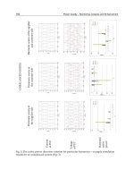
often preferable), peak-valley methods, direct comparison and normalization – all
these simple transformations cangive interesting information. One majorapplication
is, however, the exploitation of the presence of isosbestic points (IPs), when several
spectra cross together at least at a single point (Pouet et al., 2004). Depending on the
condition of the IP appearance, directly from a set of spectra (or after normalization
in the case of hidden IPs) the composition of wastewater can vary from one state to
another (qualitative conservation) with a possible quantitative conservation when a
direct IP occurs. Applications of this nonparametric measurement will be shown in
Chapter 4.2 for the calculation of industrial wastewater variability and in Chapter 5.1
for the study of discharges in receiving medium.
JWBK117-2.1 JWBK117-Quevauviller October 10, 2006 20:15 Char Count= 0
116 Sewers (Characterization and Evolution of Sewage)
2.1.4 EVOLUTION OF SEWAGE

Considering the composition of wastewater, heterogeneous and variable, always
changing with inputs of industrial discharges or fresh domestic loads, from up-
stream to the treatment plant, its evolution is evident but complex, involving, physi-
cal, physico-chemical and biological factors. Moreover, the evolution of wastewater
depends both on the design principle of the sewer systems (gravity or pressure main)
and on the climatic conditions for combine sewers (Nielsen et al., 1992). A lot of
studies have been published on the interaction of sewerage and wastewater treatment
(Kruize, 1993) and on the role of the sewer as a physical, chemical and biological
reactor (Hvitved-Jacobsen et al., 1995). All these studies have been carried out with
classical methods for wastewater quality measurement in the laboratory. However,
changes in wastewater composition can be appreciated by the measurement of on-site
parameters of interest (see above) including the estimation of variability.
2.1.4.1 Physical Factors
The first physical factor is the flow rate ratio in the case of a mixture or discharge,
playing a role in the concentration or dilution of pollutants concentration. The main
problem is for combined sewers during rain fall, with storm runoff drainage. At the
beginning of the event, particulate materials from roads, roofs and parking areas, and
also oil, salts, etc., can be carried to the sewer (particularly after a long dry weather
period) increasing the pollution load. Then, after flushing, the main phenomenon
remains dilution. The effects of storm water in combined sewers vary with the
characteristics of the sewers (length, diameters, etc.) and the topography (slope)
leading to the equalization of loads in the case of small flow rate and large volumes.
In this case, settling of large or dense particles generally occurs, and the settled
material can be flushed with the increase of flow if the sewer is combined (collecting
both wastewater and storm water runoff). Thus, the wastewater quality of long sewers
in a flat area, (partly) combined, presents huge variations and differences between dry
and wet periods. Finally, temperature variation (generally an increase) is possible
with industrial wastewater of enterprises with cooling open circuits or rejecting
hot effluent. A hot temperature leads to the increase of the kinetics of biological
and physico-chemical reactions (biodegradation, chemical reactions), mainly by the

increase of equilibrium ‘constants’ (which depend on temperature), but also by the
increase solubility of some organics (for example, the solubility of benzene in water
increases 20 % up to 1900 mg/l, between 10
◦
C and 30
◦
C). A hot temperature leads
to the evaporation of solvents for laundry discharge, for example.
2.1.4.2 Physico-chemical Factors
The first physico-chemical factor is the variation of pH responsible for the modifica-
tion of acidic–basic reactions. Even if wastewater is considered as a buffer medium
JWBK117-2.1 JWBK117-Quevauviller October 10, 2006 20:15 Char Count= 0
Evolution of Sewage 117
Table 2.1.1 Percentage of unionized ammonia with respect to pH and temperature (pK
a
= 9.25
at 25
◦
C)
pH
Temperature (
◦
C) 6.0 7.0 8.0 9.0 9.25 10.0
10 0.02 0.2 1.8 15.7 24.9 65.0
20 0.04 0.4 3.8 28.4 41.4 79.8
30 0.08 0.8 7.4 44.6 58.8 88.9
considering its composition as a complex mixture, acidic or basic shocks are locally
possible with industrial or accidental discharge of concentrated acid or base solu-
tions. One consequence can be, for example, on ammonia equilibrium (Table 2.1.1),
with the increase of the toxic form (unionized ammonia) with pH (and temperature).

For example, a concentration of ammonia of 10 mg/l at 20
◦
C and for a pH of 8.0,
gives a concentration of the unionized form equal to 0.38 mg/l, which is toxic.
Another physico-chemical factor is the redox potential E
H
, fixed by the respective
concentration of chemical oxidized and/or reduced substances. As for temperature
or pH, variations of redox conditions are related to industrial discharges. A decrease
of E
H
can give septic conditions (for example, E
H
≤ 40 mV for pH =7) leading to
odour production and sewer corrosion in the presence of sulfides (Degr´emont, 2005).
There are some other physico-chemical factors involved in sewage evolution, like
precipitation, due to pH increase (for hydroxides) or exceeding of solubility products
in the case of industrial discharge, or complexation by the presence of chelating
agents. One last important point is the fate of surfactants, the concentration of which
being high in some industrial discharges. Depending on the presence of colloids and
on flow conditions, theses substances can be adsorbed on suspended solids, leading
to the aggregation of colloids with a decrease of the dissolved amount of dispersants.
This phenomenon is responsible for sample ageing (Baur`es et al., 2004).
2.1.4.3 Biological Factors
Even if physical and physico-chemical factors of wastewater composition evolution
are numerous, the biological ones are more important. Regarding the degradation
of organic substances, where used, biological reactions in sewers are principally
anaerobic, bur aerobic conditions can be encountered in some gravity sewers. Even if
the concentration of dissolved oxygen is very low (<2 mg/l), some aerobic processes
may occur as in biological treatment plants. In the pressure part of the sewer or in the

case of high organic load, expressed by high oxygen demand values (BOD or COD),
no dissolved oxygen is available (nor in the gaseous phase, which is dangerous for
operators). Thus, the organic matter can be partially degraded through fermentation
reactions, accompanied by the chemical reduction of some minerals, like the sulfate
ion to sulfide. This reaction occurs for septic conditions (see above), and leads to
odour production and corrosion of the sewer.
JWBK117-2.1 JWBK117-Quevauviller October 10, 2006 20:15 Char Count= 0
118 Sewers (Characterization and Evolution of Sewage)
Another biological factor is the potential toxicity of a lot of substances, often
brought by industrial discharges in sewers, able to cause severe damage in the bi-
ological reactors of the wastewater treatment plant (death of active biomass). The
toxicity effect depends on the nature and concentration of substances, but also on
the existence of an acclimated biomass potentially in contact with wastewater. For
example, depending on the organisms, phenol is toxic from concentrations between
10 mg/l and 25 mg/l but concentrations up to 400 mg/l can be treated by biologi-
cal processes (Bevilacqua et al., 2002). As for the previous factors, the main cause
of wastewater quality variation and evolution (except dilution by storm runoff in
combined sewers) is the occurrence of shock loads associated with point industrial
discharges, the effects of which are important in the case of short sewers or if the
discharge is close to the treatment plant.
REFERENCES
Barcelo, D. (2005) Emerging Organic Pollutants in Wastewater and Sludge. The Handbook of
Environmental Chemistry, vol. 5, parts I and O. Springer-Verlag, Berlin.
Baur`es, E. (2002) La mesure non param´etrique, un nouvel outil pour l’´etude des effluents in-
dustriels: application aux eaux r´esiduaires d’une raffinerie. PhD Thesis, University of Aix
Marseille III.
Baur`es, E., Berho, C., Pouet, M F. and Thomas, O. (2004) Water Sci. Technol., 49(1), 47–52.
Bevilacqua, J.V., Cammarota, M.C., Freire, D.M.G. and Sant Anna, G.L. (2002) Brazilian J. Chem.
Engin., 19(2), 151–158.
Bourgeois, W., Burgess, J.E. and Stuetz, R.M. (2001) J. Chem. Technol. Biotechnol., 76, 337–348.

Colin, F. and Quevauviller, Ph. (Eds) (1998) Monitoring of Water Quality, the Contribution of
Advanced Technologies. Elsevier, Amsterdam.
Degr´emont (2005) M´emento technique de l’eau, 10th Edn. Paris.
European Commission (1991) Council Directive of 21 May 1991 concerning urban wastewater
treatment (91/271/EEC).
Fleishman, N., Langergraber, G. and Haberl R. (2003) Proceedings of the IWA International
Specialised Conference, Vienna, Austria, 21–22 May 2002. Water Sci. Technol., 47(2).
Hvitved-Jacobsen, T., Nielsen, P.H., Larsen, T. and Aa Jensen, N. (1995) Proceedings of the
International Specialised Conference, Aalborb, Denmark, 16–18 May 1994. Water Sci. Tech-
nol., 31(7).
Kruize, R.R. (1993) Proceedings of the International Conference, Amsterdam, The Netherlands,
31 August–4 September 1992. Water Sci. Technol., 27(5–6).
Nielsen, P.H., Raunkjaer, K., Norsker, N.H. and Hvitved-Jacobsen, T. (1992) Water Sci. Technol.,
25(6), 17–31.
Olsson, G., Jeppsson, U. and Rosen, C. (2002) Proceedings of the IWA International Conference,
Malm¨o, Sweden, 3–7 June 2001. Water Sci. Technol., 45(4–5).
Pouet, M F., Baur`es, E., Vaillant, S. and Thomas, O. (2004) Appl. Spectrosc., 58(4), 486–490.
Thomas, O. (1995) M´etrologie des eaux r´esiduaires. Cebedoc, Tec et Doc Lavoisier, Li`ege, Paris.
Thomas, O., El Khorassani, H., Touraud, E. and Bitar, H. (1999) Talanta, 50, 743–749.
Vaillant, S., Pouet, M F. and Thomas, O. (2002) Urban Water, 4, 273–281.
Vanrolleghem, P.A. and Lee, D.S. (2003) Water Sci. Technol., 47(2), 1–34.
JWBK117-2.2 JWBK117-Quevauviller October 10, 2006 20:18 Char Count= 0
2.2
Sewer Flow Measurement
Charles S. Melching
2.2.1 Introduction
2.2.1.1 Purposes of Flow Monitoring
2.2.1.2 Equipment Selection Considerations
2.2.1.3 Monitoring Locations
2.2.1.4 Characteristics of Ideal Sewer Flow Measurement Equipment

2.2.1.5 Quality Assurance and Quality Control
2.2.2 Manning’s Equation
2.2.3 Flumes
2.2.4 Electromagnetic Flow Meters
2.2.5 Area–Velocity Flow Meters
2.2.5.1 Narrow-beam Doppler Area–Velocity Flow Meters
2.2.5.2 Wide-beam Doppler Area–Velocity Flow Meters
2.2.5.3 Independent Evaluation of Doppler Area–Velocity Flow Meters
2.2.5.4 Summary
2.2.6 Acoustic Doppler Profiler Flow Meters
2.2.7 Comparison of Flow Measurement Techniques
2.2.8 Conclusions and Perspectives
References
2.2.1 INTRODUCTION
Sewers are difficult environments in which to obtain accurate discharge estimates
for many reasons including rapidly changing flow conditions, surcharge, backwater,
Wastewater Quality Monitoring and Treatment Edited by P. Quevauviller, O. Thomas and A. van der Beken
C

2006 John Wiley & Sons, Ltd. ISBN: 0-471-49929-3