6. Process or Product Monitoring and Control
6.2.Test Product for Acceptability: Lot
Acceptance Sampling
This section describes how to make decisions on a lot-by-lot basis
whether to accept a lot as likely to meet requirements or reject the lot as
likely to have too many defective units.
Contents of
section 2
This section consists of the following topics.
What is Acceptance Sampling?1.
What kinds of Lot Acceptance Sampling Plans (LASPs) are
there?
2.
How do you Choose a Single Sampling Plan?
Choosing a Sampling Plan: MIL Standard 105D1.
Choosing a Sampling Plan with a given OC Curve2.
3.
What is Double Sampling? 4.
What is Multiple Sampling?5.
What is a Sequential Sampling Plan?6.
What is Skip Lot Sampling?7.
6.2. Test Product for Acceptability: Lot Acceptance Sampling
[5/1/2006 10:34:45 AM]
6. Process or Product Monitoring and Control
6.2. Test Product for Acceptability: Lot Acceptance Sampling
6.2.1.What is Acceptance Sampling?
Contributions
of Dodge and
Romig to
acceptance
sampling

Acceptance sampling is an important field of statistical quality control
that was popularized by Dodge and Romig and originally applied by
the U.S. military to the testing of bullets during World War II. If every
bullet was tested in advance, no bullets would be left to ship. If, on the
other hand, none were tested, malfunctions might occur in the field of
battle, with potentially disastrous results.
Definintion of
Lot
Acceptance
Sampling
Dodge reasoned that a sample should be picked at random from the
lot, and on the basis of information that was yielded by the sample, a
decision should be made regarding the disposition of the lot. In
general, the decision is either to accept or reject the lot. This process is
called Lot Acceptance Sampling or just Acceptance Sampling.
"Attributes"
(i.e., defect
counting) will
be assumed
Acceptance sampling is "the middle of the road" approach between no
inspection and 100% inspection. There are two major classifications of
acceptance plans: by attributes ("go, no-go") and by variables. The
attribute case is the most common for acceptance sampling, and will
be assumed for the rest of this section.
Important
point
A point to remember is that the main purpose of acceptance sampling
is to decide whether or not the lot is likely to be acceptable, not to
estimate the quality of the lot.
Scenarios

leading to
acceptance
sampling
Acceptance sampling is employed when one or several of the
following hold:
Testing is destructive
●
The cost of 100% inspection is very high●
100% inspection takes too long●
6.2.1. What is Acceptance Sampling?
(1 of 2) [5/1/2006 10:34:45 AM]
Acceptance
Quality
Control and
Acceptance
Sampling
It was pointed out by Harold Dodge in 1969 that Acceptance Quality
Control is not the same as Acceptance Sampling. The latter depends
on specific sampling plans, which when implemented indicate the
conditions for acceptance or rejection of the immediate lot that is
being inspected. The former may be implemented in the form of an
Acceptance Control Chart. The control limits for the Acceptance
Control Chart are computed using the specification limits and the
standard deviation of what is being monitored (see Ryan, 2000 for
details).
An
observation
by Harold
Dodge
In 1942, Dodge stated:

" basically the "acceptance quality control" system that was
developed encompasses the concept of protecting the consumer from
getting unacceptable defective product, and encouraging the producer
in the use of process quality control by: varying the quantity and
severity of acceptance inspections in direct relation to the importance
of the characteristics inspected, and in the inverse relation to the
goodness of the quality level as indication by those inspections."
To reiterate the difference in these two approaches: acceptance
sampling plans are one-shot deals, which essentially test short-run
effects. Quality control is of the long-run variety, and is part of a
well-designed system for lot acceptance.
An
observation
by Ed
Schilling
Schilling (1989) said:
"An individual sampling plan has much the effect of a lone sniper,
while the sampling plan scheme can provide a fusillade in the battle
for quality improvement."
Control of
product
quality using
acceptance
control charts
According to the ISO standard on acceptance control charts (ISO
7966, 1993), an acceptance control chart combines consideration of
control implications with elements of acceptance sampling. It is an
appropriate tool for helping to make decisions with respect to process
acceptance. The difference between acceptance sampling approaches
and acceptance control charts is the emphasis on process acceptability

rather than on product disposition decisions.
6.2.1. What is Acceptance Sampling?
(2 of 2) [5/1/2006 10:34:45 AM]
6. Process or Product Monitoring and Control
6.2. Test Product for Acceptability: Lot Acceptance Sampling
6.2.2.What kinds of Lot Acceptance
Sampling Plans (LASPs) are there?
LASP is a
sampling
scheme and
a set of rules
A lot acceptance sampling plan (LASP) is a sampling scheme and a set
of rules for making decisions. The decision, based on counting the
number of defectives in a sample, can be to accept the lot, reject the lot,
or even, for multiple or sequential sampling schemes, to take another
sample and then repeat the decision process.
Types of
acceptance
plans to
choose from
LASPs fall into the following categories:
Single sampling plans:. One sample of items is selected at
random from a lot and the disposition of the lot is determined
from the resulting information. These plans are usually denoted as
(n,c) plans for a sample size n, where the lot is rejected if there
are more than c defectives. These are the most common (and
easiest) plans to use although not the most efficient in terms of
average number of samples needed.
●
Double sampling plans: After the first sample is tested, there are

three possibilities:
Accept the lot1.
Reject the lot2.
No decision3.
If the outcome is (3), and a second sample is taken, the procedure
is to combine the results of both samples and make a final
decision based on that information.
●
Multiple sampling plans: This is an extension of the double
sampling plans where more than two samples are needed to reach
a conclusion. The advantage of multiple sampling is smaller
sample sizes.
●
Sequential sampling plans: . This is the ultimate extension of
multiple sampling where items are selected from a lot one at a
time and after inspection of each item a decision is made to accept
or reject the lot or select another unit.
●
Skip lot sampling plans:. Skip lot sampling means that only a●
6.2.2. What kinds of Lot Acceptance Sampling Plans (LASPs) are there?
(1 of 3) [5/1/2006 10:34:46 AM]
fraction of the submitted lots are inspected.
Definitions
of basic
Acceptance
Sampling
terms
Deriving a plan, within one of the categories listed above, is discussed
in the pages that follow. All derivations depend on the properties you
want the plan to have. These are described using the following terms:

Acceptable Quality Level (AQL): The AQL is a percent defective
that is the base line requirement for the quality of the producer's
product. The producer would like to design a sampling plan such
that there is a high probability of accepting a lot that has a defect
level less than or equal to the AQL.
●
Lot Tolerance Percent Defective (LTPD): The LTPD is a
designated high defect level that would be unacceptable to the
consumer. The consumer would like the sampling plan to have a
low probability of accepting a lot with a defect level as high as
the LTPD.
●
Type I Error (Producer's Risk): This is the probability, for a
given (n,c) sampling plan, of rejecting a lot that has a defect level
equal to the AQL. The producer suffers when this occurs, because
a lot with acceptable quality was rejected. The symbol
is
commonly used for the Type I error and typical values for
range from 0.2 to 0.01.
●
Type II Error (Consumer's Risk): This is the probability, for a
given (n,c) sampling plan, of accepting a lot with a defect level
equal to the LTPD. The consumer suffers when this occurs,
because a lot with unacceptable quality was accepted. The symbol
is commonly used for the Type II error and typical values range
from 0.2 to 0.01.
●
Operating Characteristic (OC) Curve: This curve plots the
probability of accepting the lot (Y-axis) versus the lot fraction or
percent defectives (X-axis). The OC curve is the primary tool for

displaying and investigating the properties of a LASP.
●
Average Outgoing Quality (AOQ): A common procedure, when
sampling and testing is non-destructive, is to 100% inspect
rejected lots and replace all defectives with good units. In this
case, all rejected lots are made perfect and the only defects left
are those in lots that were accepted. AOQ's refer to the long term
defect level for this combined LASP and 100% inspection of
rejected lots process. If all lots come in with a defect level of
exactly p, and the OC curve for the chosen (n,c) LASP indicates a
probability p
a
of accepting such a lot, over the long run the AOQ
can easily be shown to be:
●
6.2.2. What kinds of Lot Acceptance Sampling Plans (LASPs) are there?
(2 of 3) [5/1/2006 10:34:46 AM]
where N is the lot size.
Average Outgoing Quality Level (AOQL): A plot of the AOQ
(Y-axis) versus the incoming lot p (X-axis) will start at 0 for p =
0, and return to 0 for p = 1 (where every lot is 100% inspected
and rectified). In between, it will rise to a maximum. This
maximum, which is the worst possible long term AOQ, is called
the AOQL.
●
Average Total Inspection (ATI): When rejected lots are 100%
inspected, it is easy to calculate the ATI if lots come consistently
with a defect level of p. For a LASP (n,c) with a probability p
a
of

accepting a lot with defect level p, we have
ATI = n + (1 - p
a
) (N - n)
where N is the lot size.
●
Average Sample Number (ASN): For a single sampling LASP
(n,c) we know each and every lot has a sample of size n taken and
inspected or tested. For double, multiple and sequential LASP's,
the amount of sampling varies depending on the the number of
defects observed. For any given double, multiple or sequential
plan, a long term ASN can be calculated assuming all lots come in
with a defect level of p. A plot of the ASN, versus the incoming
defect level p, describes the sampling efficiency of a given LASP
scheme.
●
The final
choice is a
tradeoff
decision
Making a final choice between single or multiple sampling plans that
have acceptable properties is a matter of deciding whether the average
sampling savings gained by the various multiple sampling plans justifies
the additional complexity of these plans and the uncertainty of not
knowing how much sampling and inspection will be done on a
day-by-day basis.
6.2.2. What kinds of Lot Acceptance Sampling Plans (LASPs) are there?
(3 of 3) [5/1/2006 10:34:46 AM]
6. Process or Product Monitoring and Control
6.2. Test Product for Acceptability: Lot Acceptance Sampling

6.2.3.How do you Choose a Single
Sampling Plan?
Two
methods for
choosing a
single
sample
acceptance
plan
A single sampling plan, as previously defined, is specified by the pair of
numbers (n,c). The sample size is n, and the lot is rejected if there are
more than c defectives in the sample; otherwise the lot is accepted.
There are two widely used ways of picking (n,c):
Use tables (such as MIL STD 105D) that focus on either the AQL
or the LTPD desired.
1.
Specify 2 desired points on the OC curve and solve for the (n,c)
that uniquely determines an OC curve going through these points.
2.
The next two pages describe these methods in detail.
6.2.3. How do you Choose a Single Sampling Plan?
[5/1/2006 10:34:46 AM]
6. Process or Product Monitoring and Control
6.2. Test Product for Acceptability: Lot Acceptance Sampling
6.2.3. How do you Choose a Single Sampling Plan?
6.2.3.1. Choosing a Sampling Plan: MIL
Standard 105D
The AQL or
Acceptable
Quality

Level is the
baseline
requirement
Sampling plans are typically set up with reference to an acceptable
quality level, or AQL . The AQL is the base line requirement for the
quality of the producer's product. The producer would like to design a
sampling plan such that the OC curve yields a high probability of
acceptance at the AQL. On the other side of the OC curve, the consumer
wishes to be protected from accepting poor quality from the producer.
So the consumer establishes a criterion, the lot tolerance percent
defective or LTPD . Here the idea is to only accept poor quality product
with a very low probability. Mil. Std. plans have been used for over 50
years to achieve these goals.
The U.S. Department of Defense Military Standard 105E
Military
Standard
105E
sampling
plan
Standard military sampling procedures for inspection by attributes were
developed during World War II. Army Ordnance tables and procedures
were generated in the early 1940's and these grew into the Army Service
Forces tables. At the end of the war, the Navy also worked on a set of
tables. In the meanwhile, the Statistical Research Group at Columbia
University performed research and outputted many outstanding results
on attribute sampling plans.
These three streams combined in 1950 into a standard called Mil. Std.
105A. It has since been modified from time to time and issued as 105B,
195C and 105D. Mil. Std. 105D was issued by the U.S. government in
1963. It was adopted in 1971 by the American National Standards

Institute as ANSI Standard Z1.4 and in 1974 it was adopted (with minor
changes) by the International Organization for Standardization as ISO
Std. 2859. The latest revision is Mil. Std 105E and was issued in 1989.
These three similar standards are continuously being updated and
revised, but the basic tables remain the same. Thus the discussion that
follows of the germane aspects of Mil. Std. 105E also applies to the
6.2.3.1. Choosing a Sampling Plan: MIL Standard 105D
(1 of 3) [5/1/2006 10:34:46 AM]
other two standards.
Description of Mil. Std. 105D
Military
Standard
105D
sampling
plan
This document is essentially a set of individual plans, organized in a
system of sampling schemes. A sampling scheme consists of a
combination of a normal sampling plan, a tightened sampling plan, and
a reduced sampling plan plus rules for switching from one to the other.
AQL is
foundation
of standard
The foundation of the Standard is the acceptable quality level or AQL. In
the following scenario, a certain military agency, called the Consumer
from here on, wants to purchase a particular product from a supplier,
called the Producer from here on.
In applying the Mil. Std. 105D it is expected that there is perfect
agreement between Producer and Consumer regarding what the AQL is
for a given product characteristic. It is understood by both parties that
the Producer will be submitting for inspection a number of lots whose

quality level is typically as good as specified by the Consumer.
Continued quality is assured by the acceptance or rejection of lots
following a particular sampling plan and also by providing for a shift to
another, tighter sampling plan, when there is evidence that the
Producer's product does not meet the agreed-upon AQL.
Standard
offers 3
types of
sampling
plans
Mil. Std. 105E offers three types of sampling plans: single, double and
multiple plans. The choice is, in general, up to the inspectors.
Because of the three possible selections, the standard does not give a
sample size, but rather a sample code letter. This, together with the
decision of the type of plan yields the specific sampling plan to be used.
Inspection
level
In addition to an initial decision on an AQL it is also necessary to decide
on an "inspection level". This determines the relationship between the
lot size and the sample size. The standard offers three general and four
special levels.
6.2.3.1. Choosing a Sampling Plan: MIL Standard 105D
(2 of 3) [5/1/2006 10:34:46 AM]
Steps in the
standard
The steps in the use of the standard can be summarized as follows:
Decide on the AQL.1.
Decide on the inspection level.2.
Determine the lot size.3.
Enter the table to find sample size code letter.4.

Decide on type of sampling to be used.5.
Enter proper table to find the plan to be used.6.
Begin with normal inspection, follow the switching rules and the
rule for stopping the inspection (if needed).
7.
Additional
information
There is much more that can be said about Mil. Std. 105E, (and 105D).
The interested reader is referred to references such as (Montgomery
(2000), Schilling, tables 11-2 to 11-17, and Duncan, pages 214 - 248).
There is also (currently) a web site developed by Galit Shmueli that will
develop sampling plans interactively with the user, according to Military
Standard 105E (ANSI/ASQC Z1.4, ISO 2859) Tables.
6.2.3.1. Choosing a Sampling Plan: MIL Standard 105D
(3 of 3) [5/1/2006 10:34:46 AM]
6. Process or Product Monitoring and Control
6.2. Test Product for Acceptability: Lot Acceptance Sampling
6.2.3. How do you Choose a Single Sampling Plan?
6.2.3.2.Choosing a Sampling Plan with a
given OC Curve
Sample
OC
curve
We start by looking at a typical OC curve. The OC curve for a (52 ,3) sampling
plan is shown below.
6.2.3.2. Choosing a Sampling Plan with a given OC Curve
(1 of 6) [5/1/2006 10:34:47 AM]
Number of
defectives is
approximately

binomial
It is instructive to show how the points on this curve are obtained, once
we have a sampling plan (n,c) - later we will demonstrate how a
sampling plan (n,c) is obtained.
We assume that the lot size N is very large, as compared to the sample
size n, so that removing the sample doesn't significantly change the
remainder of the lot, no matter how many defects are in the sample.
Then the distribution of the number of defectives, d, in a random
sample of n items is approximately binomial with parameters n and p,
where p is the fraction of defectives per lot.
The probability of observing exactly d defectives is given by
The binomial
distribution
The probability of acceptance is the probability that d, the number of
defectives, is less than or equal to c, the accept number. This means
that
Sample table
for Pa, Pd
using the
binomial
distribution
Using this formula with n = 52 and c=3 and p = .01, .02, ,.12 we find
P
a
P
d
.998 .01
.980 .02
.930 .03
.845 .04

.739 .05
.620 .06
.502 .07
.394 .08
.300 .09
.223 .10
.162 .11
.115 .12
Solving for (n,c)
6.2.3.2. Choosing a Sampling Plan with a given OC Curve
(2 of 6) [5/1/2006 10:34:47 AM]
Equations for
calculating a
sampling plan
with a given
OC curve
In order to design a sampling plan with a specified OC curve one
needs two designated points. Let us design a sampling plan such that
the probability of acceptance is 1-
for lots with fraction defective p
1
and the probability of acceptance is for lots with fraction defective
p
2
. Typical choices for these points are: p
1
is the AQL, p
2
is the LTPD
and

, are the Producer's Risk (Type I error) and Consumer's Risk
(Type II error), respectively.
If we are willing to assume that binomial sampling is valid, then the
sample size n, and the acceptance number c are the solution to
These two simultaneous equations are nonlinear so there is no simple,
direct solution. There are however a number of iterative techniques
available that give approximate solutions so that composition of a
computer program poses few problems.
Average Outgoing Quality (AOQ)
Calculating
AOQ's
We can also calculate the AOQ for a (n,c) sampling plan, provided
rejected lots are 100% inspected and defectives are replaced with good
parts.
Assume all lots come in with exactly a p
0
proportion of defectives.
After screening a rejected lot, the final fraction defectives will be zero
for that lot. However, accepted lots have fraction defectivep
0
.
Therefore, the outgoing lots from the inspection stations are a mixture
of lots with fractions defective p
0
and 0. Assuming the lot size is N, we
have.
For example, let N = 10000, n = 52, c = 3, and p, the quality of
incoming lots, = 0.03. Now at p = 0.03, we glean from the OC curve
table that p
a

= 0.930 and
AOQ = (.930)(.03)(10000-52) / 10000 = 0.02775.
6.2.3.2. Choosing a Sampling Plan with a given OC Curve
(3 of 6) [5/1/2006 10:34:47 AM]
Sample table
of AOQ
versus p
Setting p = .01, .02, , .12, we can generate the following table
AOQ p
.0010 .01
.0196 .02
.0278 .03
.0338 .04
.0369 .05
.0372 .06
.0351 .07
.0315 .08
.0270 .09
.0223 .10
.0178 .11
.0138 .12
Sample plot
of AOQ
versus p
A plot of the AOQ versus p is given below.
6.2.3.2. Choosing a Sampling Plan with a given OC Curve
(4 of 6) [5/1/2006 10:34:47 AM]
Interpretation
of AOQ plot
From examining this curve we observe that when the incoming quality

is very good (very small fraction of defectives coming in), then the
outgoing quality is also very good (very small fraction of defectives
going out). When the incoming lot quality is very bad, most of the lots
are rejected and then inspected. The "duds" are eliminated or replaced
by good ones, so that the quality of the outgoing lots, the AOQ,
becomes very good. In between these extremes, the AOQ rises, reaches
a maximum, and then drops.
The maximum ordinate on the AOQ curve represents the worst
possible quality that results from the rectifying inspection program. It
is called the average outgoing quality limit, (AOQL ).
From the table we see that the AOQL = 0.0372 at p = .06 for the above
example.
One final remark: if N >> n, then the AOQ ~ p
a
p .
The Average Total Inspection (ATI)
Calculating
the Average
Total
Inspection
What is the total amount of inspection when rejected lots are screened?
If all lots contain zero defectives, no lot will be rejected.
If all items are defective, all lots will be inspected, and the amount to
be inspected is N.
Finally, if the lot quality is 0 < p < 1, the average amount of inspection
per lot will vary between the sample size n, and the lot size N.
Let the quality of the lot be p and the probability of lot acceptance be
p
a
, then the ATI per lot is

ATI = n + (1 - p
a
) (N - n)
For example, let N = 10000, n = 52, c = 3, and p = .03 We know from
the OC table that p
a
= 0.930. Then ATI = 52 + (1 930) (10000 - 52) =
753. (Note that while 0.930 was rounded to three decimal places, 753
was obtained using more decimal places.)
6.2.3.2. Choosing a Sampling Plan with a given OC Curve
(5 of 6) [5/1/2006 10:34:47 AM]
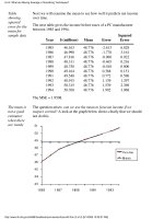
Sample table
of ATI versus
p
Setting p= .01, .02, 14 generates the following table
ATI P
70 .01
253 .02
753 .03
1584 .04
2655 .05
3836 .06
5007 .07
6083 .08
7012 .09
7779 .10
8388 .11
8854 .12
9201 .13
9453 .14

Plot of ATI
versus p
A plot of ATI versus p, the Incoming Lot Quality (ILQ) is given below.
6.2.3.2. Choosing a Sampling Plan with a given OC Curve
(6 of 6) [5/1/2006 10:34:47 AM]
6. Process or Product Monitoring and Control
6.2. Test Product for Acceptability: Lot Acceptance Sampling
6.2.4.What is Double Sampling?
Double Sampling Plans
How double
sampling
plans work
Double and multiple sampling plans were invented to give a questionable lot
another chance. For example, if in double sampling the results of the first
sample are not conclusive with regard to accepting or rejecting, a second
sample is taken. Application of double sampling requires that a first sample of
size n
1
is taken at random from the (large) lot. The number of defectives is then
counted and compared to the first sample's acceptance number a
1
and rejection
number r
1
. Denote the number of defectives in sample 1 by d
1
and in sample 2
by d
2
, then:

If d
1
a
1
, the lot is accepted.
If d
1
r
1
, the lot is rejected.
If a
1
< d
1
< r
1
, a second sample is taken.
If a second sample of size n
2
is taken, the number of defectives, d
2
, is counted.
The total number of defectives is D
2
= d
1
+ d
2
. Now this is compared to the
acceptance number a

2
and the rejection number r
2
of sample 2. In double
sampling, r
2
= a
2
+ 1 to ensure a decision on the sample.
If D
2
a
2
, the lot is accepted.
If D
2
r
2
, the lot is rejected.
Design of a Double Sampling Plan
6.2.4. What is Double Sampling?
(1 of 5) [5/1/2006 10:34:47 AM]
Design of a
double
sampling
plan
The parameters required to construct the OC curve are similar to the single
sample case. The two points of interest are (p
1
, 1- ) and (p

2
, , where p
1
is the
lot fraction defective for plan 1 and p
2
is the lot fraction defective for plan 2. As
far as the respective sample sizes are concerned, the second sample size must
be equal to, or an even multiple of, the first sample size.
There exist a variety of tables that assist the user in constructing double and
multiple sampling plans. The index to these tables is the p
2
/p
1
ratio, where p
2
>
p
1
. One set of tables, taken from the Army Chemical Corps Engineering
Agency for
= .05 and = .10, is given below:
Tables for n
1
= n
2
accept approximation values
R = numbers of pn
1
for

p
2
/p
1
c
1
c
2
P = .95 P = .10
11.90 0 1 0.21 2.50
7.54 1 2 0.52 3.92
6.79 0 2 0.43 2.96
5.39 1 3 0.76 4.11
4.65 2 4 1.16 5.39
4.25 1 4 1.04 4.42
3.88 2 5 1.43 5.55
3.63 3 6 1.87 6.78
3.38 2 6 1.72 5.82
3.21 3 7 2.15 6.91
3.09 4 8 2.62 8.10
2.85 4 9 2.90 8.26
2.60 5 11 3.68 9.56
2.44 5 12 4.00 9.77
2.32 5 13 4.35 10.08
2.22 5 14 4.70 10.45
2.12 5 16 5.39 11.41
Tables for n
2
= 2n
1

accept approximation values
R = numbers of pn
1
for
p
2
/p
1
c
1
c
2
P = .95 P = .10
14.50 0 1 0.16 2.32
8.07 0 2 0.30 2.42
6.48 1 3 0.60 3.89
6.2.4. What is Double Sampling?
(2 of 5) [5/1/2006 10:34:47 AM]
5.39 0 3 0.49 2.64
5.09 0 4 0.77 3.92
4.31 1 4 0.68 2.93
4.19 0 5 0.96 4.02
3.60 1 6 1.16 4.17
3.26 1 8 1.68 5.47
2.96 2 10 2.27 6.72
2.77 3 11 2.46 6.82
2.62 4 13 3.07 8.05
2.46 4 14 3.29 8.11
2.21 3 15 3.41 7.55
1.97 4 20 4.75 9.35

1.74 6 30 7.45 12.96
Example
Example of
a double
sampling
plan
We wish to construct a double sampling plan according to
p
1
= 0.01 = 0.05 p
2
= 0.05 = 0.10 and n
1
= n
2
The plans in the corresponding table are indexed on the ratio
R = p
2
/p
1
= 5
We find the row whose R is closet to 5. This is the 5th row (R = 4.65). This
gives c
1
= 2 and c
2
= 4. The value of n
1
is determined from either of the two
columns labeled pn

1
.
The left holds
constant at 0.05 (P = 0.95 = 1 - ) and the right holds
constant at 0.10. (P = 0.10). Then holding constant we find pn
1
= 1.16 so n
1
= 1.16/p
1
= 116. And, holding constant we find pn
1
= 5.39, so n
1
= 5.39/p
2
=
108. Thus the desired sampling plan is
n
1
= 108 c
1
= 2 n
2
= 108 c
2
= 4
If we opt for n
2
= 2n

1
, and follow the same procedure using the appropriate
table, the plan is:
n
1
= 77 c
1
= 1 n
2
= 154 c
2
= 4
The first plan needs less samples if the number of defectives in sample 1 is
greater than 2, while the second plan needs less samples if the number of
defectives in sample 1 is less than 2.
ASN Curve for a Double Sampling Plan
6.2.4. What is Double Sampling?
(3 of 5) [5/1/2006 10:34:47 AM]
Construction
of the ASN
curve
Since when using a double sampling plan the sample size depends on whether
or not a second sample is required, an important consideration for this kind of
sampling is the Average Sample Number (ASN) curve. This curve plots the
ASN versus p', the true fraction defective in an incoming lot.
We will illustrate how to calculate the ASN curve with an example. Consider a
double-sampling plan n
1
= 50, c
1

= 2, n
2
= 100, c
2
= 6, where n
1
is the sample
size for plan 1, with accept number c
1
, and n
2
, c
2
, are the sample size and
accept number, respectively, for plan 2.
Let p' = .06. Then the probability of acceptance on the first sample, which is the
chance of getting two or less defectives, is .416 (using binomial tables). The
probability of rejection on the second sample, which is the chance of getting
more than six defectives, is (1 971) = .029. The probability of making a
decision on the first sample is .445, equal to the sum of .416 and .029. With
complete inspection of the second sample, the average size sample is equal to
the size of the first sample times the probability that there will be only one
sample plus the size of the combined samples times the probability that a
second sample will be necessary. For the sampling plan under consideration,
the ASN with complete inspection of the second sample for a p' of .06 is
50(.445) + 150(.555) = 106
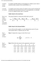
The general formula for an average sample number curve of a double-sampling
plan with complete inspection of the second sample is
ASN = n
1

P
1
+ (n
1
+ n
2
)(1 - P
1
) = n
1
+ n
2
(1 - P
1
)
where P
1
is the probability of a decision on the first sample. The graph below
shows a plot of the ASN versus p'.
The ASN
curve for a
double
sampling
plan
6.2.4. What is Double Sampling?
(4 of 5) [5/1/2006 10:34:47 AM]
6.2.4. What is Double Sampling?
(5 of 5) [5/1/2006 10:34:47 AM]
6. Process or Product Monitoring and Control
6.2. Test Product for Acceptability: Lot Acceptance Sampling

6.2.5.What is Multiple Sampling?
Multiple
Sampling is
an extension
of the
double
sampling
concept
Multiple sampling is an extension of double sampling. It involves
inspection of 1 to k successive samples as required to reach an ultimate
decision.
Mil-Std 105D suggests k = 7 is a good number. Multiple sampling plans
are usually presented in tabular form:
Procedure
for multiple
sampling
The procedure commences with taking a random sample of size n
1
from
a large lot of size N and counting the number of defectives, d
1
.
if d
1
a
1
the lot is accepted.
if d
1
r

1
the lot is rejected.
if a
1
< d
1
< r
1
, another sample is taken.
If subsequent samples are required, the first sample procedure is
repeated sample by sample. For each sample, the total number of
defectives found at any stage, say stage i, is
This is compared with the acceptance number a
i
and the rejection
number r
i
for that stage until a decision is made. Sometimes acceptance
is not allowed at the early stages of multiple sampling; however,
rejection can occur at any stage.
Efficiency
measured by
the ASN
Efficiency for a multiple sampling scheme is measured by the average
sample number (ASN) required for a given Type I and Type II set of
errors. The number of samples needed when following a multiple
sampling scheme may vary from trial to trial, and the ASN represents the
average of what might happen over many trials with a fixed incoming
defect level.
6.2.5. What is Multiple Sampling?

(1 of 2) [5/1/2006 10:34:48 AM]