JWBK117-2.3 JWBK117-Quevauviller October 10, 2006 20:18 Char Count= 0
158 Monitoring in Rural Areas
this means that the system is not as fully automated as some might hope and that
regular visits to the stations by employees should be foreseen. Also, a too complex
‘black-box’ concept of the system leads to a significant loss of data. The processing
of the sensor signal to data should be transparent showing what can be done by using
PC-based modulesforthecontrolofthe station.Aweb-basedcommunication enables
remote control of the stations and the integration of the data into databases. This
concept also allows for a full remote control of the station by authorised persons and
a limited accessibility for data consultation by users through the web. A better spatial
representation can be obtained by embedding the monitoring and the modelling in a
GIS system (Vivoni and Richards, 2005).
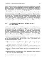
2.3.4 CONCLUSIONS AND PERSPECTIVES
Monitoring in rural areas needs a different approach than in urban areas. The pollu-
tion in rural areas cannot be measured at certain points along the water body, but can
only be estimated by making evaluations of the water quality together with infor-
mation on what and how many polluting substances are applied in the area. Models,
describing all processes on those substances before entering the water, can provide
a means to evaluate the magnitude of pollution coming from diffuse pollution and
to evaluate scenarios for diffuse pollution reduction. Specific data are needed to
calibrate and build those models.
Therefore, the traditional cycle in water management should be inversed. Instead
of starting from the data set to select an appropriate tool and hence use this tool for
management, one should first define the problem, select a tool that can support this
problem and then design an appropriate monitoring program to feed the tool. In that
way, money is spent to generate primarily the information that is indeed needed. A
closer cooperation between monitoring and modelling efforts will make sure that
models for diffuse pollution can be used with sufficient reliability.
Automated monitoring can help to catch the high variability or short rain-driven
events. Such tools can only provide reliable data provided that the monitoring system
is transparent and follows quality control procedures with regard to maintenance and

calibration. While a high level of automation may support such procedures, it still
requires considerable manpower that should be foreseen in any monitoring budget.
REFERENCES
Arnold, J.G., Williams, J.R., Srinivasan, R. and King, K.W. (1996) SWAT Manual. USDA, Agri-
cultural Research Service and Blackland Research Center, Texas.
Barthelemy, P.A. and Vidal, C. (1999) A dynamic European agricultural and agri-foodstuff sec-
tor. In: Agriculture, Environment, Rural Development, Facts and Figures – A Challenge for
Agriculture. European Commission Report, Belgium.
Beck, M.B. (1987) Water Resour. Res., 23(8), 1393.
JWBK117-2.3 JWBK117-Quevauviller October 10, 2006 20:18 Char Count= 0
References 159
Bervoets, L., Schneiders, A. and Verheyen, R.F. (1989) Onderzoek naar de verspreiding en de
typologie van ecologisch waardevolle waterlopen in het Vlaams gewest. Deel 1 - Het Dender-
bekken, Universitaire Instelling Antwerpen. In Dutch.
Boschma, M., Joaris, A. and Vidal, C. (1999) Concentrations of livestock production. In: Agri-
culture, Environment, Rural Development, Facts and Figures – A Challenge for Agriculture.
European Commission Report, Belgium.
Brown, L.C. and Barnwell T.O. (1987) The Enhanced Stream Water Quality Models QUAL2E and
QUAL2E-UNCAS: Documentation and User Model. EPA/600/3-87/007, USA.
Janssen, P.H.M., Heuberger, P.S.C. and Sanders,S. (1992) ManualUncsam 1.1, aSoftware Package
for Sensitivity and Uncertainty Analysis. Bilthoven, The Netherlands.
Krysanova, V. and Haberlandt, U. (2001) Ecol. Modelling, 150, 255–275.
McKay, M.D. (1988) Sensitivity and uncertainty analysis using a statistical sample of input values.
In: Uncertainty Analysis, Y. Ronen, ed. CRC Press, Inc., Boca Raton, FL, pp. 145–186.
Montarella, L. (1999) Soil at the interface between agriculture and environment. In: Agriculture,
Environment, Rural Development, Facts and Figures – A Challenge for Agriculture. European
Commission Report, Belgium.
Pau Val, M. and Vidal, C. (1999) Nitrogen in agriculture. In: Agriculture, Environment, Rural
Development, Facts and Figures – A Challenge for Agriculture. European Commission Report,
Belgium.

Poirot, M. (1999) Crop trends and environmental impacts. In: Agriculture, Environment, Rural
Development, Facts and Figures – A Challenge for Agriculture. European Commission Report,
Belgium.
Sevruk, B. (1986) Proceedings of the ETH, IAHS International Workshop on the Correction of
Precipitation Measurements, 1–3 April 1985. ETH Z¨urich, Z¨uricher Geographische Schriften,
Z¨urich, p. 23.
Smets, S. (1999) Modelling of nutrient losses in the Dender catchment using SWAT. Masters
dissertation. Katholieke Universiteit Leuven –Vrije Universiteit, Brussels, Belgium.
Vandenberghe, V., van Griensven, A. and Bauwens, W. (2005) Water Sci.Technol., 51(3-4), 347–
354.
Vandenberghe, V., Goethals, P., van Griensven, A., Meirlaen, J., De Pauw, N., Vanrolleghem, P.A.
and Bauwens, W. (2004) Environ. Monitor Assess., 108, 85–98.
van Griensven, A. and Bauwens, W. (2001) Water Sci. Technol., 43(7), 321–328.
van Griensven, A. and Bauwens, W. (2003) Water Resour. Res., 39(10), 1348.
van Griensven, A., Vandenberghe, V. and Bauwens, W. (2002) Proceedings of the International
IWA Conference on Automation in Water Quality Monitoring, 21–22, May 2002. Vienna,
Austria.
Vivoni, E.R. and Richards, K.T. (2005) J. Hydroinform., 7(4), 235–250.
JWBK117-3.1 JWBK117-Quevauviller October 10, 2006 20:25 Char Count= 0
3.1
Elements of Modelling and
Control of Urban Wastewater
Treatment Systems
Olivier Potier and Marie-No¨elle Pons
3.1.1 Introduction
3.1.2 Short Description of the Biological Process by Activated Sludge
3.1.3 Process Parameters
3.1.3.1 Biokinetics
3.1.3.2 Oxygen Transfer
3.1.3.3 Hydrodynamics

3.1.3.4 Wastewater Variability
3.1.3.5 Mass Balance
3.1.4 Sensors
3.1.4.1 In-line Sensors
3.1.4.2 On-line Sensors
3.1.5 Introduction to the Control Methods of a Wastewater Treatment Plant
by Activated Sludge
3.1.6 Conclusion and Perspectives
Acknowledgement
References
Wastewater Quality Monitoring and Treatment Edited by P. Quevauviller, O. Thomas and A. van der Beken
C

2006 John Wiley & Sons, Ltd. ISBN: 0-471-49929-3
JWBK117-3.1 JWBK117-Quevauviller October 10, 2006 20:25 Char Count= 0
162 Elements of Modelling andControlof Urban Wastewater Treatment Systems
3.1.1 INTRODUCTION
A wastewater treatment plant (WWTP) is an intricate system made of unit operations
based on physical, biological and physico-chemical principles. Its aim is principally
the removal of organic, nitrogen and phosphorus pollution. The basic processes are
complex and the various arrangements of the unit operations which can be proposed
lead to many possible configurations of WWTPs. It is difficult to describe in detail
all of the processes here and only the basics of biological treatment by activated
sludge will be examined. It is the most widespread for WWTPs of medium and
large size. The interested reader will find more details in Henze et al. (Henze et al.,
2000). We focus our attention on the most important parameters for optimization
and process control of pollution removal in large plants, where spatial distribution of
substrate and nutrient in the reacting system plays a large role. In smaller plants, time
scheduling can replace spatial gradients as in sequencing batch reactors for example.
Whatever the case and in spite of the perturbations in terms of flow, composition and

concentration experienced at the inletof any WWTP, specificationson the discharged
water should be kept within strict limits to avoid taxes and penalties. Different tools
for monitoring and process control are also presented.
3.1.2 SHORT DESCRIPTION OF THE BIOLOGICAL
PROCESS BY ACTIVATED SLUDGE
The biological step (often called secondary treatment) is an essential part of the
WWTP. At the inlet of the plant, the water is usually pretreated to remove gross
debris (grit removal) and can be further treated in a primary settler, which will elim-
inate a large part (usually 40–50 %) of the particulate pollution. In doing so, part of
the biodegradable pollution is indeed removed, which might not always be a good
idea: denitrification, one of the steps involved in nitrogen pollution removal, requires
a certain balance between carbon and nitrogen and an external carbon source is often
added in that step. This could be avoided (or at least limited) by direct injection into
the biological reactor of unsettled wastewater. The principle of activated sludge is the
intensification in a reactor of the principle of self-purification, which is naturally oc-
curring in the environment, in presence of a much higher bacterial concentration than
in rivers or lakes. The task of the secondary clarifier (Figure 3.1.1) is to separate the
biological reactor by
activated sludge
return sludge
purified
water
clarifier
Figure 3.1.1 Schematic representation of an activated sludge system
JWBK117-3.1 JWBK117-Quevauviller October 10, 2006 20:25 Char Count= 0
Process Parameters 163
aerobic zone
anoxic
zone
Post-denitrification

aerobic zone
anoxic
zone
Pre-denitrification
C
Figure 3.1.2 Schemes of different activated sludge reactors with anoxic zone
flocculated bacteria (sludge flocs) from the treated water. The sludge is returned to
the inlet of the reactor and the purified water is polished in a tertiary stage (post-
treatment of phosphorus, filtration, disinfection, etc.) and/or discharged.
In the presence of oxygen, carbon and a small amount of nitrogen (from ammonia
and hydrolysed organic nitrogen) are metabolizedby heterotrophic biomass and most
of the nitrogen by autotrophic bacteria. The latter produced nitrates can be reduced
by heterotrophs under anoxic conditions. As indicated previously, organic matter
is needed for this reaction and therefore an addition of carbon (such as methanol)
is often necessary. In the case of a pre-denitrification system, mixed liquor from
the outlet of the reactor is recycled to the anoxic zone. Some of the most classical
schemes are presented in Figure 3.1.2.
In order to ensure the best process efficiency, different parameters must be known
and controlled: the main reactions of pollution removal and their kinetics; the spatial
distribution of the substrates with respect to the micro-organisms and therefore the
reactor hydrodynamics; the aeration capacity and therefore the oxygen transfer; and
the variability of thewastewater,in terms ofcomposition,concentrationand flowrate.
3.1.3 PROCESS PARAMETERS
3.1.3.1 Biokinetics
Many differentcompoundsand micro-organismsarefoundin a biologicalwastewater
system. In addition, the ecosystem is never at steady state. Therefore, an exact and
complete kinetic model is out of reach. For many years the scientific community has
tried to provide models of reasonable complexity, able to describe the main steps
of activated sludge behaviour. The basic model is ASM1 (Activated Sludge Model
n

◦
1), devoted to carbon and nitrogen removal (Henze et al., 1987). Improved versions
have been proposed, such as ASM2, which takes into account phosphorus removal,
and ASM3 (IWA, 2000).
ASM1 is a good compromise between the description of the complex reality of
biological reactions and the simplicity of a model. The identification of any model
parameter should be possible theoretically (structural identifiability) and experimen-
tally through experiments which can be run in the laboratory as well as on full-scale
systems.
JWBK117-3.1 JWBK117-Quevauviller October 10, 2006 20:25 Char Count= 0
164 Elements of Modelling andControlof Urban Wastewater Treatment Systems
S
s
S
o
X
s
X
p
S
NH
S
I
X
I
X
B,H
X
B,A
X

ND
S
ND
S
NO
r
3
r
4
r
3
r
3
r
6
r
8
r
5
r
5
r
5
r
4
r
4
r
2
r

2
r
2
r
7
r
1
r
1
r
1
S
I

: Soluble inert organic matter
S
s
: readily biodegradable substrate
X
s
: Slowly biodegradable substrate
X
I
: Particulate inert organic matter
X
B,H
: Active heterotrophic biomass
X
B,A
: Active autotrophic biomass

X
p
: Particulate products arising from biomass decay
S
o
: Oxygen
S
NO
: Nitrate and nitrite nitrogen
S
NH
: NH
4
+
and NH
3
nitrogen
S
ND
: Soluble biodegradable organic nitrogen
X
ND
: Particulate biodegradable organic nitrogen
Figure 3.1.3 Schematic representation of the ASM1 kinetic pathways
As ASM1 is more particularly used, it will be described in some detail. In ASM1
(Figure 3.1.3), wastewater compounds are divided into different categories: inert (i.e.
nonbiodegradable) versus biodegradable matter, particulate versus soluble. Partic-
ulate biodegradable matter should be hydrolysed to become readily biodegradable.
The biomass is divided into two parts: heterotrophic and autotrophic.
Note that toxic events could trigger strong inhibition of bacteria. Inhibition terms

can be added to the basic ASM1 model for specific purpose (industrial wastewater
mainly). Autotrophs are deemed to be more sensitive to toxics than heterotrophs.
3.1.3.2 Oxygen Transfer
Influence of oxygen on pollution removal
Bacteria use oxygen for their respiration. In the ASM1 model, the oxygen concen-
tration is considered to be a substrate:
r
For the aerobic growth of heterotrophs, where readily biodegradable substrate is
consumed:
ρ
1
= μ
H

S
S
K
S
+ S
S

S
O
K
O,H
+ S
O

X
B,H

where ρ
1
is the aerobic growth rate of heterotrophs, S
S
the biodegradable soluble
substrate concentration, S
O
the oxygen concentration, X
B,H
the concentration of
heterotrophs, K
S
the heterotrophic half-saturation coefficient for S
S
, K
O,H
the het-
erotrophic half-saturation/inhibition coefficient for oxygen and μ
H
the maximum
growth rate of heterotrophs.
JWBK117-3.1 JWBK117-Quevauviller October 10, 2006 20:25 Char Count= 0
Process Parameters 165
r
For the aerobic growth of autotrophs, where NH
4
+
and NH
3
nitrogen are trans-

formed into nitrates:
ρ
3
= μ
A

S
NH
K
NH
+ S
NH

S
O
K
O,A
+ S
O

X
B,A
where ρ
3
is the aerobic growth rate of autotrophs, S
NH
the ammonium concen-
tration, X
B,A
the concentration of autotrophs, K

NH
the autotrophic half-saturation
coefficient for S
NH
, K
O,A
the autotrophic half-saturation coefficient for oxygen
and μ
A
the maximum growth rate of heterotrophs.
For the anoxic growth of heterotrophs, a very low concentration of oxygen is
required to avoid any inhibition:
ρ
2
= μ
H

S
S
K
S
+ S
S

K
O,H
K
O,H
+ S
O


S
NO
K
NO
+ S
NO

η
g
X
B,H
where ρ
2
is the anoxic growth rate of heterotrophs, S
NO
the nitrate concentration,
K
NO
the heterotrophic half-saturation coefficient for S
NO
and η
g
the anoxic growth
rate correction factor for heterotrophs.
Thus, the oxygen concentration has a great importance: it should be low in the
anoxic stages and nonlimiting in the aerated zones. However, excessive oxygen
supply should be penalized in terms of cost. Oxygen is provided by gas diffusers or
surface aerators.
Oxygen transfer model

Generally, the gas–liquid transfer is modelled by means of the double film theory
(Roustan et al., 2003), according to which the gas–liquid interface is located between
a gas film and a liquid film. For the oxygen–water system, the transfer resistance is
found in the liquid film, due to the low solubility of oxygen in water. The oxygen
flux is a function of the difference between the oxygen concentration at saturation
(S
∗
O
) and the dissolved oxygen concentration in the reactor
(
S
O
)
and of the global
coefficient of oxygen transfer (k
L
a

). Experimental values of k
L
a

are generally
between 2 h
−1
and 10 h
−1
. If it is assumed that the reactor can be modelled as a
Continuous Perfectly Mixed Reactor (CPMR) (Figure 3.1.4), with a uniform oxygen
concentration, the oxygen mass balance is written as:

QS
OI
+ k
L
a

(S
∗
O
− S
O
)V = QS
O
+r
O
V + V
dS
O
dt
with S
OI
the oxygen concentration at the inlet, r
O
the oxygen consumption rate, V
the reactor volume and Q the liquid flow rate.
The coefficient transfer is measured directly in the presence of sludge (k
L
a

), or

in clean water without sludge (k
L
a)(H´eduit and Racault, 1983a,b; ASCE, 1992;
JWBK117-3.1 JWBK117-Quevauviller October 10, 2006 20:25 Char Count= 0
166 Elements of Modelling andControlof Urban Wastewater Treatment Systems
air
water inlet water outlet
QS
OI
QS
O
S
O
Figure 3.1.4 An aerated Continuous Perfectly Mixed Reactor
Roustan et al., 2003). In this case, the so-called ‘alpha’ factor (α) must be taken into
account (Boumansour and Vasel, 1996):
k
L
a

= αk
L
a
Example of oxygen profile in a WWTP bioreactor
To illustrate the open loop behaviour of a biological reactor, with no aeration adjust-
ment as a function of the oxygen demand, the oxygen profile was measured during
1 day in a 3300 m
3
channel reactor with a large aspect ratio. The reactor is 100 m
long and 8 m wide and aerated by means of fine bubble diffusers located on its floor.

The dissolved oxygen concentration was regularly measured in six locations along
the reactor with a portable probe (WTW, Weilheim, Germany) (Figure 3.1.5). The
1.8
0.8
0.6
0.4
0.2
0
0 5 10 15 20 25 30
1.6
1.4
1.2
1
time/h
dissolved oxygen/mg L
−
1
O
2
(near inlet)
O
2
(1/8 of the length)
O
2
(1/3 of the length)
O
2
(1/2 of the length)
O

2
(2/3 of the length)
O
2
(near outlet)
Figure 3.1.5 Variations of the dissolved oxygen concentration in different locations of an acti-
vated sludge channel reactor during 1 day
JWBK117-3.1 JWBK117-Quevauviller October 10, 2006 20:25 Char Count= 0
Process Parameters 167
air flow rate was constant and equally distributed along the reactor, which was con-
tinuously fed by urban presettled wastewater. The dissolved oxygen concentration
changes with the oxygen consumption, and therefore with biodegradable pollution
concentration, which depends on time and space in the reactor.
In Figure 3.1.5, it can be seen that dissolved oxygen concentration is higher
during the night, when pollution is lower. The concentration increases along the
reactor as the oxygen consumption decreases due to a decrease in the biodegradable
substrate availability. During the day, dissolved oxygen concentration remains very
low, even near the reactor outlet, which indicates complete pollution removal is not
achieved. Under such conditions oxygen limitation occurs. Better aeration with a
larger air flow rate could alleviate such a limitation without increasing the reactor
volume.
3.1.3.3 Hydrodynamics
In brief, two types of reactor shape are found: a compact, ‘parallelepipedic’ or
‘cylindrical’ design, often fitted with surface turbines for aeration; and an elongated
design suitable for gas diffusion devices. Elongated reactors are often folded or
built as ‘race tracks’, which avoids recirculation pumps (Figure 3.1.6). In this case
they are generally called ‘oxidation ditches’ when the aerators are horizontal and
‘carousels’ when they are vertical. Many variations have been proposed by various
manufacturers, such as sets of several concentric channels as in the Orbal
TM

sys-
tem and OCO
TM
process, inclusion of anaerobic and anoxic zones equipped with
mechanical mixing devices, or combination of spatial gradients along the tanks
with alternating mode of operation, such as in the Biodenipho
TM
or Biodenitro
TM
process. Capacity, land availability, flow circulation, process type (carbon and/or
nutrient removal) are some of the criteria for selection.
Hydrodynamics haveagreat importance in a process, because linked withkinetics,
they affect pollution removal efficiency and the bacteria species selectivity. Usually
the reactor behaviour is compared with one of two ideal types: the Continuous
Perfectly Mixed Reactor (or CPMR) and the Plug Flow Reactor.
The CPMR is characterized by a uniform concentration of each component in all
the volume of the reactor. This type of reactor can be found in small WWTPs, where
the length is similar to the width.
aerobic and
anoxic zone
Figure 3.1.6 A ‘race track’ reactor
JWBK117-3.1 JWBK117-Quevauviller October 10, 2006 20:25 Char Count= 0
168 Elements of Modelling andControlof Urban Wastewater Treatment Systems
123
J
Q Q
Figure 3.1.7 J CPMRs in series
The Plug Flow Reactor model is very different. It is composed of a succession of
parallel volumes infinitiely small, perpendicular to the flow, with no transfer between
them. These volumes move forward from the inlet to the outlet, at a velocity linearly

related to the flow. There is a progressive change in concentrations. However, if the
ideal Plug Flow Reactor model could be used for tubular or fixed-bed reactors in the
chemical industry, it rarely represents in a satisfactory manner an aerated tank in a
WWTP.
Models based on CPMRs in series (Figure 3.1.7) offerthebestsimplealternative to
model full-scale plants and generally give a good agreement with experimental data.
Theoretically, the number of reactors in series (J) can vary between 1 and infinity. In
practice, J is determined by tracing experiments and takes values between 3 and 20.
Although a series of J CPMRs is a discrete hydrodynamic model, it can model a
continuous liquid system like a channel reactor.
Hydrodynamic characterization
A relatively simple method for the characterization of hydrodynamics is the Resi-
dence Time Distribution (RTD) method. Each molecule has is own residence time
(r
t
) in the reactor, which depends on the reactor hydrodynamics (Figure 3.1.8). The
goal of the RTD method is to measure the different residence times based on statis-
tics. A pulse of nonreactive tracer is injected at the inlet of the reactor. Different
chemical substances are used, such as lithium chloride (detection by atomic ab-
sorption), rhodamine (detection by fluorescence sensor) and radioactive elements.
The tracer is dissolved in the mixed liquor in the reactor and behaves as the liquid
phase. At the reactor outlet, the tracer concentration is measured to calculate the
RTD (Villermaux, 1993; Levenspiel, 1999).
Inlet signal Outlet signal
Figure 3.1.8 Inert tracing of a reactor
JWBK117-3.1 JWBK117-Quevauviller October 10, 2006 20:25 Char Count= 0
Process Parameters 169
0
0 0.5 1.5 2.5123
0.2

0.4
0.6
0.8
1.0
1.2
1.4
1.6
1.8
2.0
q
=
r
t

t
−
1
E

=

E
(
r
t
)
t
J = 20
J = 10
J = 6

J = 4
J = 3
J = 2
J = 1
Figure 3.1.9 Theoretical RTD tracings of different sets of CPMRs in series
For CPMRs in series, the RTD is a function of J and of the space time τ = V/Q:
E(r
t
) =

J
τ

J
r
t
J−1
exp
(
−Jr
t
/τ
)
(
J −1
)
!
In Figure 3.1.9, theoretical RTD tracings for series of J CPMRs (J = 1–20) are
plotted. The parameters are normalized by the space time τ.
Influence of hydrodynamics on pollution removal

In biological wastewater treatment, kinetics are a function of the biodegradable
substrate concentration (S
S
); the larger the concentration, the larger the reaction
rates. In this case, it can be demonstrated that better pollution removal efficiency is
obtained with CPMRs in series than with a single CPMR. The larger the J, the better
the efficiency. Therefore, between two reactors with the same volume, the better one
is the longest.
Moreover,inactivated sludge, filamentous bacteria, whichconstitutethebackbone
of activated sludge flocs, could overgrow, which creates a problem called filamentous
bulking. This problem has many causes, but it has been noticed that the hydrody-
namics of a CPMR favours this phenomenon (Chudoba et al., 1973). Conversely,
a reactor with a high aspect ratio, behaving as a series of CPMRs favours a more
‘normal’, i.e. well balanced, biomass. It is a problem of selectivity.
JWBK117-3.1 JWBK117-Quevauviller October 10, 2006 20:25 Char Count= 0
170 Elements of Modelling andControlof Urban Wastewater Treatment Systems
Computer Fluid Dynamics
Computer Fluid Dynamics (CFD) is a recent tool used to analyse in detail the flow
characteristics in a number of systems, including chemical and biological reactors
(Ranade, 2002). However, many hurdles remain, especially in the field of wastewater
treatment. Assumptions concerning limit and initial conditions, turbulence model,
etc., should be made. Activated sludge processes are multiphase systems but the
liquid and ‘solid’ (biomass) phases are generally considered as a single homogenous
liquid in which the bubbles (gas phase) are in motion. Two approaches are generally
utilized to simulate this gas–liquid system. The Euler approach is used in both cases
for the liquid phase. The gas phase can be treated by a Eulerian approach (Euler–
Euler) or a Lagrangian approach (Euler–Lagrange). There is a third method, Volume
of Fluid (VOF), but this is generally only used for small systems with few bubbles.
In spite of the increase in computer speed and the possible parallelization of some
calculations, the simulation time remains very long and it is still difficult to introduce

mass transfer and kinetics in this type of simulation.
3.1.3.4 Wastewater Variability
Different types of variability
Wastewater characteristics change with time, not only in terms of flow rate, but
also in terms of composition and concentration. Wastewater variability depends on
human and industrial activities and on weather conditions, especially in combined
sewernetworkswhere sewage is mixed with run-offwater from roofs, pavements, etc.
Several scales ofdry-weather variability are recognized: daily, weekly and seasonally
disturbances affect the wastewater characteristics.
Example of variability
Figure 3.1.10 illustrates the variability of chemical oxygen demand (COD) at the
inlet of the wastewater treatment system of a 2000 inhabitants’ community in France,
under summer dry weather conditions. A 24-h period is clearly visible. Week days
(Monday through Friday) present a similar pattern, where morning, lunchtime and
evening activities induce COD peaks. In weekend days pollution is higher as in-
habitants tend to remain at home and are not going to work in the nearby large
city. In large urban centres the trend will be the opposite, with less pollution during
weekends than week days.
Flow rate variability and its influence on hydrodynamics
Reactor hydrodynamics are affected by the diurnal flow rate variations. Fig-
ure 3.1.11 presents the example of the flow characteristics at the inlet of a 350 000
JWBK117-3.1 JWBK117-Quevauviller October 10, 2006 20:25 Char Count= 0
Process Parameters 171
1600
1200
800
400
0
24/6 25/6 26/6 27/6 28/6 29/6 30/6 1/7 2/7 3/7
Tue Wen Thu Fri Sam Sun Mon

COD
/
mg
.
L
−
1
Figure 3.1.10 Example of COD variations in a 2000 inhabitants’ community
person-equivalent plant. The effect of rain can also be seen in the middle of the week.
Part of the incoming wastewater was bypassed and directly discharged to the river,
which explained the limitation at 6500 m
3
/h.
RTDs were determined in the channel reactors previously described under dif-
ferent flow conditions and they show that the tanks can be modelled by CPMRs in
series. The hydrodynamic behaviour is modified by the flow rate and the number of
CPMRs (Figure 3.1.12), J, changes with the space-time τ, and therefore with the
water flow rate Q (Potier et al., 2005):
J =
L
2
2 τ D
+ 1 and τ =
V
Q
where L is the reactor length.
or J =
K
τ
+ 1 with K =

L
2
2 D
8000
6000
4000
2000
0
flow rate
/
m
3
h
−
1
08/28/01 08/30/01 09/01/01 09/03/01
Tue Wen Thu Fri Sam Sun Mon
Figure 3.1.11 Flow rate variations, at the inlet of a 350 000 person-equivalent WWTP
JWBK117-3.1 JWBK117-Quevauviller October 10, 2006 20:25 Char Count= 0
172 Elements of Modelling andControlof Urban Wastewater Treatment Systems
30
25
20
15
10
40 60 80 100 120 140 160 180 200
5
0
J (full scale plant)
J (pilot plant)

t

/

min
J
Figure 3.1.12 Number of CPMRs (J ) versus liquid space-time (τ ) for a full-scale plant and a
bench-scale plant
Often, hydrodynamics are considered as a fixed parameter. In order to facilitate
the modelling task, it is convenient to work with a constant number of CPMRs. By
introducing the concept of CPMRs in series with back-mixing (Figure 3.1.13), a
compromise is reached.
12 3 J
max
Q
Q
(
b+1
)
Q
b Q
Figure 3.1.13 Schematic representation of CPMRs in series with back-mixing
A maximum number of cells, J
max
, is assumed for a given reactor. The model
corresponds to different apparent J values (J
app
) varying from 1 to J
max
, de-

pending on the back-mixing flow (βQ) and on J
max
according to the following
relationship:
β =
1
2

(
J
max
− 1
)
−

1 + J
2
max

1 −
2
J
app

1/2

which is valid for J
app
larger than 2.5.
3.1.3.5 Mass Balance

The full mass balance enables finally to bring together the different aspects: hydro-
dynamics, kinetics and mass transfer. It is the basis of the global model used for the
JWBK117-3.1 JWBK117-Quevauviller October 10, 2006 20:25 Char Count= 0
Sensors 173
understanding of the system, its simulation, its optimization and even its automation.
The first stage is to identify the hydrodynamic model, as described previously. For
a CPMR, a mass balance equation is then written for each component (substrates,
metabolites). For CPMRs in series, a mass balance equation is necessary for each
component in each CPMR.
3.1.4 SENSORS
Many different sensors are foundonWWTPs. They give information abouttreatment
efficiency and they are necessary to monitor, control and optimize the processes
(Vanrolleghem and Lee, 2003; Degr´emont, 2005). There are three types of sensors:
in-line sensors situated directly in the process; on-line sensors, based on automated
sampling and conditioning of the sample; and off-line devices, in plant laboratories,
which require human operators. In any case in-line and on-line sensors will require
careful maintenance, including automated cleaning sequences, and calibration.
3.1.4.1 In-line Sensors
In-line sensors are mostly devoted to physical parameters: flow rate [water, gases (air,
methane from sludge digesters, etc.), sludge, reagents such as polymers for sludge
conditioning, precipitants such asion chloride for phosphorus removal], level (liquid,
sludge blanket), pressure, temperature, electrical power, suspended solids, turbidity,
etc. A few chemical sensors are also available such as pH, redox, dissolved oxygen,
conductivity, ammonia (with an ion-selective probe). More recently devices based on
UV-visible spectrophotometry have been proposed as surrogate measurements for
COD, which requires a 2 h digestion. These systems operate at a fixed wavelength
(254 nm in general) or collect spectra in the range 200–600 nm (Spectro::lyser,
Scan Messtechnik GmbH, Vienna, Austria). Fluorescence sensors (BioView, Delta
Light & Optics, Denmark) and infrared technology (Steyer et al., 2002) offer also
new prospectsfor in-situ wastewater qualitymonitoring based on spectroscopy (Pons

et al., 2004).
3.1.4.2 On-line Sensors
On-line sensors have been proposed for nitrate, ammonia, phosphate, short-term
biological oxygen demand (BOD) (to evaluate the oxygen demand and control the
aeration rate), toxicity (based on bacterial respiration) (Vanrolleghem et al., 1994)
and sludge volume index (to detect settling problems such as filamentous bulking)
(Vanderhasselt et al., 1999).
JWBK117-3.1 JWBK117-Quevauviller October 10, 2006 20:25 Char Count= 0
174 Elements of Modelling andControlof Urban Wastewater Treatment Systems
3.1.5 INTRODUCTION TO THE CONTROL METHODS
OF A WASTEWATER TREATMENT PLANT BY
ACTIVATED SLUDGE
The aims of control systems are to maintain the concentration and the flux of pollu-
tants below the limits fixed by the environmental norms and to reduce the operating
costs. WWTPs are often designed so as to operate near their limits in order to
minimize the investment costs. Therefore they become more sensitive to inlet per-
turbations. It is even more the case for nutrient removal systems which are more
easily disturbed by an ammonia / carbon inbalance than carbon removal plants.
In some cases treatment capacity increases up to 25 % can be obtained by carefully
designed control strategies, without increasing the reactor volume. Within Europe,
the level of implementation of instrumentation, control and automation systems
varies depending on the country (Jeppsson et al., 2002; Olsson et al., 2005).
WWTPs are very complex to control because of the composition and the time
variability of the biomass and the wastewater. As shown previously, their mod-
els need many parameters, are nonstationary and strongly nonlinear. Many control
strategies, presenting different degrees of sophistication, have been proposed but
they are often difficult to test and validate at full-scale. For this reason a bench-
marking procedure, initiated at the European level in COST Actions (Jeppsson
and Pons, 2004) and further developed in an IWA Task Group, has been proposed
(). In many cases, the control techniques used in

WWTPs are simple and pragmatic.
The open loop combined with some time scheduling is the simple‘control’system.
For example, for the aeration of the activated sludge, the air flow rate can be set to a
lower value during the night than during the day. Because of disturbances, this basic
control method gives limited results.
When a valve or a pump manipulation is triggered by a measurement provided
by some sensor situated after the controlled process, the system works in closed
loop. In feedback control the measured variable is compared with a set point
(Figure 3.1.14). A control law, usually of the PID (proportional-integral-derivative)
error
non measured
disturbances
CONTROLLER
setpoint
Control
law
−1
Σ
measurement
PROCESS
Figure 3.1.14 Schematic representation of a basic feedback control loop
JWBK117-3.1 JWBK117-Quevauviller October 10, 2006 20:25 Char Count= 0
Introduction to the Control Methods of a Wastewater Treatment Plant 175
or PI (proportional-integral) type (Corriou, 2004), transforms the resulting error into
information for the actuator (situated before the controlled process), which has an
action on the process. Three types of actuator operations can be found: on/off, con-
tinuous or discrete. When possible feedforward control, which causes the system to
react before the perturbations could have effects on the plant, should be implemented:
for example, the inlet flow rate variations can be used to predict the variability of
the incoming load.

In some small plants a unique reactor is used with alternated periods of aeration
and anoxia. The phase durations are deduced from the measurement and the control
of the dissolved oxygen. Better results are obtained, if this information is com-
bined with a nitrate or a redox potential sensor (Chachuat et al., 2005; Fikar et al.,
2005).
In larger reactors, the anoxic reaction and the aeration are taking place in different
zones. In the aeration tank, the controlled variable can be the dissolved oxygen and
the actuator the valve controlling the air flow (Olsson et al., 2005). To illustrate our
purpose, a schematic representation of a 600 000 person equivalent WWTP control
system is shown in Figure 3.1.15. There are three lines and each line is divided into
two parts. Each part is controlled by a cascade of two PIDs. Sensor redundancy is
provided by two dissolved oxygen (DO) probes.
Nitrate concentration can be controlled by the addition of an external carbon
source, in order to keep the correct ratio between nitrate and carbon during denitrifi-
cation or by adjustment of the internal recycle flow in a pre-denitrification scenario
(Gernaey and Jørgensen 2004).
The control loops can be independent but in general interactions between them
exist and make the life of the control engineer difficult. They can be organized in a
hierarchical control system. The basic control loops are taken care of at the lowest
level, close to the process. Their setpoints are defined at a higher level. In the event
selection of
sensor 1 or
2 or average
manuel setpoint
of flow rate
setpoint of
flow rate
Auto 1 Auto 2
PID
(slow)

PID
DO
measure 2
DO
measure 1
Aeration tank
selection
manual or
automatic
Air flow rate
measure
position actuator
4-20 mA
Aerated
zone A
line 1
Aerated
zone B
line 1
Aerated
zone A
line 2
Aerated
zone B
line 2
Aerated
zone A
line 3
Aerated
zone B

line 3
flow rate
control valves
flow rate
measures
pressure
measure
pressure control
valves
compressors
Air production unit
Figure 3.1.15 Schematic representation of a closed loop aeration control in a 600 000 person
equivalent WWTP in France (Courtesy of Degr´emont)
JWBK117-3.1 JWBK117-Quevauviller October 10, 2006 20:25 Char Count= 0
176 Elements of Modelling andControlof Urban Wastewater Treatment Systems
of a problem (such as a sensor or actuator fault), the automated control system could
be stopped and the WWTP be controlled manually, from the upper level.
3.1.6 CONCLUSION AND PERSPECTIVES
New approaches of control are proposed, but must be more widely tested in WWTPs.
Different techniques are available such as fuzzy control, internal model control,
which requires biological and hydrodynamical models, and adaptive control, which
permits on-line identification of the model parameters. However, managers are of-
ten reluctant to implement such sophisticated control strategies, as they are under
the constant pressure of achieving stricter quality limits on the discharged water,
while minimizing operation cost. The availability of a plant-scale dynamic model
representing in sufficient detail the behaviour of WWTPs and that can be used to
‘benchmark’ control strategies (Jeppsson and Pons, 2004) could help the modern-
ization of plants from the control point of view.
ACKNOWLEDGEMENT
The authors wish to thank Degr´emont and particularly Eric Garcin, Fran¸coise

Petitpain-Perrin, Jean-Pierre Hazard and Didier Perrin.
REFERENCES
ASCE (1992) Standard Measurement of Oxygen Transfer in Clean Water. American Society of
Civil Engineers, Reston, VA.
Boumansour, B.E. and Vasel, J.L. (1996) Tribune de l’eau, 5–6, 31–40.
Chachuat, B., Roche, N. and Latifi, M.A. (2005) Chem. Engin. Proc., 44, 591–604.
Chudoba, J., Ottava, V. and Madera, V. (1973. Water Res., 7, 1163–1182.
Corriou, J.P. (2004). Process Control. Springer, Berlin.
Degr´emont (2005) M´emento technique de l’eau, 10th Edn. Lavoisier SAS.
Fikar, M., Chachuat, B. and Latifi, M.A. (2005) Control Engin. Pract., 13, 853–861.
Gernaey, K. and Jørgensen, S.B. (2004) Control Engin. Pract., 12, 357–373.
H´eduit, A. and Racault, Y. (1983a) Water Res., 17, 97–103.
H´eduit, A. and Racault, Y. (1983b) Water Res., 17, 289–297.
Henze, M., Grady, C., Gujer, W., Marais, G. and Matsuo, T. (1987) Activated sludge model no.1.
IAWPRC Task Group Report. IWA, London.
Henze, M., Harrem¨oes, P., La Cour Jansen, J. and Arvin, E. (2000) Wastewater Treatment. Bio-
logical and Chemical Processes, 3rd Ed. Springer, Berlin.
IWA (2000) Task group on mathematical modelling for design and operation of biological wastew-
ater treatment, Activated sludge models ASM1, ASM2, ASM2D and ASM3. Scientific and
Technical Report no. 9. IWA, London.
Jeppsson, U., Alex, J., Pons, M.N., Spanjers, H. and Vanrolleghem, P.A. (2002) Water Sci. Technol.,
45 (4–5), 485–494.
JWBK117-3.1 JWBK117-Quevauviller October 10, 2006 20:25 Char Count= 0
References 177
Jeppsson, U. and Pons, M.N. (2004) Control Engin. Pract., 12, 299–304.
Langergraber, G., Fleischmann, N. and Hofst¨adter, F. (2003) Water Sci. Technol., 47 (2), 63–71.
Levenspiel, O. (1999) Chemical Reaction Engineering, 3rd Edn. John Wiley & Sons, Inc., New
York.
Olsson, G., Nielsen, M.K., Yuan, Z,. Lynggaard A. and Steyer, J.P. (2005) Instrumentation, control
and automation in wastewater systems. Scientific and Technical Report no. 15. IWA Publishing,

London.
Pons, M.N. (1992) Physical and chemical sensors – actuators. In: Bioprocess Monitoring and
Control, M.N. Pons, ed. Hanser Publishers, New York.
Pons, M.N., Le Bont´e, S. and Potier, O. (2004) J. Biotechnol., 113, 211–230.
Potier, O., Leclerc, J.P. and Pons, M.N. (2005) Water Res., 39, 4454–4462.
Ranade, V.V. (2002) Computational Flow Modelling for Chemical Reactor Engineering. Process
systems engineering. Academic Press, San Diego, CA.
Roustan, M., Wild, G., H´eduit, A., Capela, S. and Gillot, S. (2003) Transfert gaz-liquide dans les
proc´ed´es de traitement des eaux et des effluents gazeux. Tec & Doc Editions, Paris.
Steyer, J.P., Bouvier, J.C., Conte, T., Gras, P., Harmand, J. and Delgenes, J.P. (2002) Water Sci.
Technol., 45 (10), 133–138.
Vanderhasselt, A., Aspegren, H., Vanrolleghem, P.A. and Verstraete, W. (1999) Water SA, 25,
453–458.
Vanrolleghem, P.A., Kong, Z., Rombouts, G. and Verstraete, W. (1994) J. Chem. Technol. Biotech-
nol., 59, 321–333.
Vanrolleghem, P.A. and Lee, D.S. (2003) Water Sci. Technol., 47(2), 1–34.
Villermaux J. (1993) G´enie de la r´eaction chimique. Lavoisier, Paris.