Multivariate Models and Algorithms for Learning Correlation Structures from Replicated Molecular Profiling Data 11
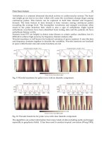
LL LM LH MM MH
rho = 0.2
rho = 0.4
M
S
E Ratio
0.00.51.01.52.0
Fig. 2. Comparison of the multivariate blind-case model and bivariate Pearson’s correlation
estimator. In the figure, the x-axis corresponds to data quality and y-axis represents MSE
ratio, which is the ratio MSE from Pearson’s estimator/MSE from blind-case model. Pair of
genes, each with 4 replicated measurements across 20 samples, were considered in the
comparison. The between molecular correlation parameter (rho) was set at 0.2 (low) and 0.4
(medium), respectively.
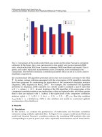
the unconstrained EM algorithm presented above may not necessarily converge to the MLE
ˆ
Ψ. To reduce various problems associated with the convergence of EM algorithm, remedies
have been proposed by constraining the eigenvalues of the component correlation matrices
(Ingrassia, 2004; Ingrassia & Rocci, 2007). For example, the constrained EM algorithm
presented in (Ingrassia, 2004) considers two strictly positive constants a and b such that
a/b
≥ c, where c ∈ (01]. In each iteration of the EM algorithm, if the eigenvalues of the
component correlation matrices are smaller than a, they are replaced with a and if they greater
than b, they are replaced with b. Indeed, if the eigenvalues of the component correlation
matrices satisfy a
≤ λ
j
(Σ
i
) ≤ b, for i = 1, 2, j = 1, 2, . . . ,
∑

k
i
=1
m
i
, then the condition
λ
min
(Σ
1
Σ
−1
2
) ≥ c (Hathaway, 1985) is also satisfied, and results in constrained (global)
maximization of the likelihood.
5. Results
5.1 Simulations
In this section, we evaluate the performance of multivariate and bivariate correlation
estimators using synthetic replicated data. In Figure 2, we compare multivariate blind-case
model and bivariate Pearson’s correlation estimator by simulating 1000 synthetic data sets
corresponding to a pair of genes, each with 4 replicated measurements and 20 observations.
51
Multivariate Models and Algorithms for
Learning Correlation Structures from Replicated Molecular Profiling Data
12 Will-be-set-by-IN-TECH
LL LM LH MM MH
B
I
−log2
(

P
)
0 5 10 15 20 25
LL LM LH MM MH
B
I
−log2
(
P
)
0 5 10 15 20 25
LL LM LH MM MH
B
I
−log2
(
P
)
0 5 10 15 20 25
LL LM LH MM MH
B
I
−log2
(
P
)
0 5 10 15 20 25
Fig. 3. Comparison of the multivariate blind-case model and informed-case model with
increasing data quality and sample size, as presented in (Zhu et al., 2010). Pair of genes, each
with 3 biological replicates and 2 technical replicates nested within a biological replicate,

were considered in the comparison. The range of between-molecular correlation parameters
was set at M (0.3-0.5). Two upper panels correspond to replicated data with sample size
n
= 20 (left) and n = 30 (right), and the lower panels correspond to the ones with n = 40
(left) and n
= 50 (right).
52
Advanced Biomedical Engineering
Multivariate Models and Algorithms for Learning Correlation Structures from Replicated Molecular Profiling Data 13
LL LM LH MM MH
B
I
−log2
(
P
)
02468101214
LL LM LH MM MH
B
I
−log2
(
P
)
02468101214
Fig. 4. Comparison of the multivariate blind-case model and informed-case model with
increasing number of technical replicates, as presented in (Zhu et al., 2010). Pair of genes,
each with 3 biological replicates and 20 observations were considered in the comparison. The
range of between-molecular correlation parameters was set at M (0.3-0.5). The left and right
panels correspond to 1 and 2 technical replicates nested within a biological replicate,

respectively.
Along the x-axis, L (low: 0.1
− 0.3), M (medium: 0.3 − 0.5) and H (high: 0.5 − 0.7) represent the
range of within-molecular correlations for each of the two genes. The y-axis corresponds to
MSE (mean squared error) ratio, which is the ratio of MSE from Pearson’s estimator over MSE
from blind-case model. Thus, MSE ratio greater than 1 indicates the superior performance
of blind-case model. We fixed the between molecular correlation parameter at 0.2 (low) and
0.4 (medium), respectively. As shown in Fig. 2, all examined MSE ratios were found greater
than 1. Figure 2 also demonstrates that the performance of blind-case model is a decreasing
function of data quality. This observation makes blind-case model particularly suitable for
analyzing real-world replicated data sets, which are often contaminated with excessive noise.
Figure 3 and Figure 4 represent parts of more detailed studies conducted in (Zhu et al., 2010)
to evaluate the performances of multivariate correlation estimators. For instance, Figure 3
compares the multivariate blind-case model and informed-case model with increasing data
quality and sample size. Synthetic data sets corresponding to a pair of genes, each with
3 biological replicates and 2 technical replicates nested within a biological replicate in 20
experiments were used in the comparison. The model performances were estimated in
terms of
− log
2
(P) values. Higher − log
2
(P) values indicate better performance by a model.
As demonstrated in Fig. 3, informed-case model significantly outperformed the blind-case
model in estimating pairwise correlation from replicated data with informed replication
mechanisms. It is also observed in Figure 3 that blind-case and informed-case models are
increasing functions of sample size and decreasing functions of data quality. The two models
were also compared in terms of increasing number of technical replicates of a biological
replicate, as demonstrated in Figure 4. We conclude from Figure 4 that blind-case and
informed-case models are decreasing functions of the number of technical replicates nested

with a biological replicate.
53
Multivariate Models and Algorithms for
Learning Correlation Structures from Replicated Molecular Profiling Data
14 Will-be-set-by-IN-TECH
LL ML HL LM MM HM MH HH
MSE

R
a
ti
o
0.0 0.5 1.0 1.5 2.0
G=2 G=3 G=4 G=8
Fig. 5. Comparison of the multivariate blind-case model and two-component finite mixture
model in terms of MSE ratio, as presented in (Acharya & Zhu, 2009). MSE ratio is calculated
as MSE from blind-case model/MSE from mixture model. Gene sets with 2, 3, 4 and 8 genes,
each with 4 replicated measurements across 20 samples were considered in the comparison.
Fig. 5, originally from (Acharya & Zhu, 2009), compares the performance of blind-case model
and two component finite mixture model in estimating the correlation structure of a gene
set. The constrained component in the mixture model corresponds to blind-case correlation
estimator. Fig. 5 plots the model performances in terms of MSE ratio defined as MSE from
blind-case model/MSE from mixture model. The number of genes in a gene set are fixed at
G
= 2, 3, 4 and 8. In Fig. 5, almost all examined MSE ratios greater than 1 indicate an overall
better performance of the mixture model approach compared with blind-case model. Fig. 5
also indicates that the performance of finite mixture model is a decreasing functions of data
quality and number of genes in the input.
5.2 Real-world data analysis
In Figure 6-8, we present real-world studies conducted in (Acharya & Zhu, 2009), where

blind-case model and finite mixture model were used to analyze two publically available
replicated data sets, spike-in data from Affymetrix () and
yeast galactose data ( />from (Yeung et al., 2003). Spike-in data comprises of the gene expression levels of 16 genes
54
Advanced Biomedical Engineering
Multivariate Models and Algorithms for Learning Correlation Structures from Replicated Molecular Profiling Data 15
0 20406080
0.00 0.05 0.10 0.15
Index of Probe Pairs
S
quared Error
Blind−case Model
Mixture Model
Fig. 6. Comparison of two multivariate models, blind-case model and finite mixture model,
in estimating pairwise correlations among genes in spike-in data, as presented in (Acharya &
Zhu, 2009).
in 20 experiments, where 16 replicated measurements are available for a gene. Correlation
structures estimated using spike-in data were compared with the nominal correlation
structure obtained from a prior known probe-level intensities. On the other hand, yeast
data contains the gene expression levels of 205 genes, each with 4 replicated measurements.
Yeast data was used to assess model performances in hierarchial clustering by utilizing a prior
knowledge of the class labels of 205 genes.
Figure 6 compares the performance of blind-case model and mixture model in estimating
pairwise correlation between genes present in spike-in data. We observed that for almost
82% of the probe pairs, mixture model provided a better approximation to the nominal
pairwise correlation compared with blind-case model. The two models were further
employed to estimate the correlation structure of a gene set. Figure 7 corresponds to the
correlation structure of a collection of 10 randomly selected probe sets from spike-in data.
As demonstrated in Figure 7, an overall better performance of mixture model approach was
given by lower squared error in comparison to blind-case model.

Finally, blind-case model and mixture model were utilized to estimate the correlation
structures from 150 subsets of yeast data, each with 60 randomly selected probe sets. The
estimated correlation structures were used to perform correlation based hierarchial clustering.
Figure 8 compares the clustering performance of blind-case model and mixture model in
terms of Minkowski score. Minkowski score is defined as
C − T/T, where C and T
are binary matrices constructed from the predicted and true labels of genes, respectively. C
ij
55
Multivariate Models and Algorithms for
Learning Correlation Structures from Replicated Molecular Profiling Data
16 Will-be-set-by-IN-TECH
0 10203040
0.0 0.2 0.4 0.6
Index of Probe Pairs
Squared Error
Blind−case Model
Mixture Model
Fig. 7. Comparison of the multivariate blind-case model and finite mixture model in
estimating the correlation structure of a gene set, as presented in (Acharya & Zhu, 2009). The
figure corresponds to a gene set comprising of 10 randomly selected probe sets in spike-in
data. Each index along the x-axis represents a probe set pair and y-axis plots squared error
values in estimating nominal correlations.
=1, if i
th
and j
th
gene belong to the same cluster in the solution and 0 otherwise. Matrix
T is obtained analogously using the true labels. A lower Minkowski score indicates higher
clustering accuracy. In Figure 8, an overall better performance of two-component mixture

model approach was observed in almost 73% cases.
6. Conclusions
Rapid developments in high-throughput data acquisition technologies have generated vast
amounts of molecular profiling data which continue to accumulate in public databases. Since
such data are often contaminated with excessive noise, they are replicated for a reliable
pattern discovery. An accurate estimate of the correlation structure underlying replicated
data can provide deep insights into the complex biomolecular activities. However, traditional
bivariate approaches to correlation estimation do not automatically accommodate replicated
measurements. Typically, an ad hoc step of data preprocessing by averaging (weighted,
unweighted or something in between) is needed. Averaging creates a strong bias while
reducing variance among the replicates with diverse magnitudes. It may also wipe out
56
Advanced Biomedical Engineering
Multivariate Models and Algorithms for Learning Correlation Structures from Replicated Molecular Profiling Data 17
0 50 100 150
1.00 1.05 1.10 1.15
Index of Gene Set
Minkowski
S
core
Blind−case Model
Mixture Model
Fig. 8. Performance of the multivariate blind-case model and finite mixture model in
clustering yeast data, as presented in (Acharya & Zhu, 2009). Each index along the x-axis
corresponds to a subset of yeast data comprising of 60 randomly selected probe sets. The
y-axis plots model performances in terms of Minkowski score. An overall better performance
of the mixture model approach is given by lower Minkowski scores in almost 73% cases.
important patterns of small magnitudes or cancel out patterns of similar magnitudes. In
many cases prior knowledge of the underlying replication mechanism might be known.
However, this information can not be exploited by averaging replicated measurements. Thus,

it is necessary to design multivariate approaches by treating each replicate as a variable.
In this chapter, we reviewed two bivariate correlation estimators, Pearson’s correlation and
SD-weighted correlation, and three multivariate models, blind-case model, informed-case
model and finite mixture model to estimate the correlation structure from replicated molecular
profiling data corresponding to a gene set with blind or informed replication mechanism. Each
of the three multivariate models treat a replicated measurement individually as a random
variable by assuming that data as independently and identically distributed samples from a
multivariate normal distribution. Blind-case model utilizes a constrained set of parameters
to define the correlation structure of a gene set with blind replication mechanism, whereas
informed-case model generalizes blind-case model by incorporating prior knowledge of
experimental design. Finite mixture model presents a more general approach of shrinking
between a constrained model, either blind-case model or informed-case model, and the
unconstrained model. The aforementioned multivariate models were used to analyze
synthetic and real-world replicated data sets. In practice, the choice of a multivariate
correlation estimator may depend on various factors, e.g. number of genes, number of
57
Multivariate Models and Algorithms for
Learning Correlation Structures from Replicated Molecular Profiling Data
18 Will-be-set-by-IN-TECH
replicated measurements available for a gene, prior knowledge of experimental design etc.
For instance, blind-case and informed-case models are more stable and computationally more
efficient than iterative EM based finite mixture model approach. However, considering
the real-world scenarios, finite mixture model assumes a more faithful representation of
the underlying correlation structure. Nonetheless, the multivariate models presented here
are sufficiently generalized to incorporate both blind and informed replication mechanisms,
and open new avenues for future supervised and unsupervised bioinformatics researches
that require accurate estimation of correlation, e.g. gene clustering, gene networking and
classification problems.
7. References
Acharya LR and Zhu D (2009). Estimating an Optimal Correlation Structure from Replicated

Molecular Profiling Data Using Finite Mixture Models. In the Proceedings of IEEE
International Conference on Machine Learning and Applications, 119-124.
Altay G and Emmert-Streib F (2010). Revealing differences in gene network inference
algorithms on the network-level by ensemble methods. Bioinformatics, 26(14),
1738-1744.
Anderson TW (1958). An introduction to mutilvariate statistical analysis, Wiley Publisher, New
York.
Basso K, Margolin AA, Stolovitzky G, Klein U, Dalla-Favera R and Califano, A (2005). Reverse
engineering of regulatory networks in human B cells. Nature Genetics, 37:382-390.
Boscolo R, Liao J, Roychowdhury VP (2008). An Information Theoretic Exploratory Method
for Learning Patterns of Conditional Gene Coexpression from Microarray Data.
IEEE/ACM Transactions on Computational Biology and Bioinformatics, 15-24.
Butte AJ and Kohane IS (2000). Mutual information relevance networks: functional genomic
clustering using pairwise entropy measurements. Pacific Symposium on Biocomputing,
5, 415-426.
Casella G and Berger RL (1990). Statistical inference, Duxbury Advanced Series.
Dempster AP, Laird NM and Rubin DB (1977). Maximum Likelihood from incomplete data
via the EM algorithm. Journal of the Royal Statistical Society B, 39(1):1-38.
Eisen M, Spellman P, Brown PO, Botstein D (1998). Cluster analysis and display of
genome-wide expression patterns. Proceedings of the National Academy of Sciences,
95:14863-14868.
Fraley C and Raftery AE (2002). Model-based clustering, discriminant analysis, and density
estimation. Journal of the American Statistical Association, 97, 611-631.
Gunderson KL, Kruglyak S, Graige MS, Garcia F, Kermani BG, Zhao C, Che D, Dickinson
T, Wickham E, Bierle J, Doucet D, Milewski M, Yang R, Siegmund C, Haas J, Zhou
L, Oliphant A, Fan JB, Barnard S and Chee MS (2004). Decoding randomly ordered
DNA arrays. Genome Research, 14:870-877.
Hastie T, Tibshirani R and Friedman J (2009). The Elements of Statistical Learning: Prediction,
Inference and Data Mining, Springer-Verlag, New York.
Hathaway RJ (1985). A constrained formulation of maximum-likelihood estimation for normal

mixture distributions. Annals of Statistics, 13, 795-800.
de Hoon MJL, Imoto S, Nolan J and Miyano S (2004). Open source clustering software.
Bioinformatics, 20(9):1453-1454.
58
Advanced Biomedical Engineering
Multivariate Models and Algorithms for Learning Correlation Structures from Replicated Molecular Profiling Data 19
Hughes TR, Marton MJ, Jones AR, Roberts CJ, Stoughton R, Armour CD, Bennett HA, Coffey
E, Dai H and He YD (2000). Functional discovery via a compendium of expression
profiles. Cell, 102:109-126.
Ingrassia S (2004). A likelihood-based constrained algorithm for multivariate normal mixture
models. Statistical Methods and Applications, 13, 151-166.
Ingrassia S and Rocci R (2007). Constrained monotone EM algorithms for the finite mixtures
of multivariate Gaussians. Computational Statistics and Data Analysis, 51, 5399-5351.
Kerr MK and Churchill GA (2001). Experimental design for gene expression microarrays.
Biostatistics, 2:183-201.
Kung C, Kenski DM, Dickerson SH, Howson RW, Kuyper LF, Madhani HD, Shokat KM (2005).
Chemical genomic profiling to identify intracellular targets of a multiplex kinase
inhibitor. Proceedings of the National Academy of Sciences, 102:3587-3592.
Lockhart DJ, Dong H, Byrne MC, Follettie MT, Gallo MV, Chee MS, Mittmann M,
Wang C, Kobayashi M, Horton H and Brown EL (1996). Expression monitoring
by hybridization to high-density oligonucleotide arrays. Nature Biotechnology,
14:1675-1680.
McLachlan GJ and Peel D (2000). Finite Mixture Models. Wiley series in Probability and
Mathematical Statistics, John Wiley & Sons.
McLachlan GJ and Peel D (2000). On computational aspects of clustering via mixtures of
normal and t-components. Proceedings of the American Statistical Association, Bayesian
Statistical Science Section, Indianapolis, Virginia.
Medvedovic M and Sivaganesan S (2002). Bayesian infinite mixture model based clustering of
gene expression profiles. Bioinformatics, 18:1194-1206.
Medvedovic M, Yeung KY and Bumgarner RE (2004). Bayesian mixtures for clustering

replicated microarray data. Bioinformatics, 20:1222-1232.
Rengarajan J, Bloom BR and Rubin EJ (2005). From The Cover: Genomewide requirements for
Mycobacterium tuberculosis adaptation and survival in macrophages. Proceedings of
the National Academy of Sciences, 102(23):8327-8332.
Sartor MA, Tomlinson CR, Wesselkamper SC, Sivaganesan S, Leikauf GD and Medvedovic, M
(2006) Intensity-based hierarchical Bayes method improves testing for differentially
expressed genes in microarray experiments. BMC Bioinformatics, 7:538.
Schäfer J and Strimmer K (2005). A shrinkage approach to large-scale covariance matrix
estimation and implications for functional genomics. Statistical Applications in
Genetics and Molecular Biology, 4, Article 32.
Shendure J and Ji H (2008). Next-generation DNA sequencing. Nature Biotechnology, 26,
1135-1145.
van’t Veer LJ, Dai HY, van de Vijver MJ, He YDD, Hart AAM, Mao M, Peterse HL, van der
Kooy K, Marton MJ, Witteveen AT, Schreiber GJ, Kerkhoven RM, Roberts C, Linsley
PS, Bernards R, Friend SH (2002). Gene expression profiling predicts clinical outcome
of breast cancer. Nature, 415:530-536.
Yao J, Chang C, Salmi ML, Hung YS, Loraine A and Roux SJ (2008). Genome-scale cluster
analysis of replicated microarrays using shrinkage correlation coefficient. BMC
Bioinformatics, 9:288.
Yeung KY, Medvedovic M and Bumgarner R. (2003). Clustering gene expression data with
repeated measurements. Genome Biology, 4:R34.
Yeung KY and Bumgarner R (2005). Multi-class classification of microarray data with repeated
measurements: application to cancer. Genome Biology, 6(405).
59
Multivariate Models and Algorithms for
Learning Correlation Structures from Replicated Molecular Profiling Data
20 Will-be-set-by-IN-TECH
Zhu D, Hero AO, Qin ZS and Swaroop A (2005). High throughput screening co-expressed
gene pairs with controlled biological significance and statistical significance. Journal
of Computational Biology, 12(7):1029-1045.

Zhu D, Li Y and Li H (2007). Multivariate correlation estimator for inferring functional
relationships from replicated genome-wide data. Bioinformatics, 23(17):2298-2305.
Zhu D and Hero AO (2007). Bayesian hierarchical model for large-scale covariance matrix
estimation. Journal of Computational Biology, 14(10):1311-1326.
Zhu D, Acharya LR and Zhang H (2010). A Generalized Multivariate Approach to Pattern
Discovery from Replicated and Incomplete Genome-wide Measurements, IEEE/ACM
transaction on Computational Biology and Bioinformatics, (in press).
60
Advanced Biomedical Engineering
4
Biomedical Time Series
Processing and Analysis Methods:
The Case of Empirical Mode Decomposition
Alexandros Karagiannis
1
,
Philip Constantinou
1
and Demosthenes Vouyioukas
2

1
National Technical University of Athens, School of Electrical and Computer Engineering,
Mobile RadioCommunication Laboratory
2
University of the Aegean,
Department of Information and Communication Systems Engineering
Greece
1. Introduction
1.1 Typical measurement systems chain

Computational processing and analysis of biomedical signals applied on the time series
follow a chain of finite number of processes. Typical schemes front process is the acquisition
of signal via the sensory subsystem. Next steps in the acquisition processing and analysis
chain include buffers and preamplifiers, the filtering stage, the analog-digital conversion
part, the removal of possible artifacts, the event detection and the analysis and feature
extraction. Figure 1 depicts this process.

Transducer
Preamplifier
Filter/
Amplifier
A/D
conversion
Signal Acquisition
Event Analysis –
Feature Extraction
Pattern
Recognition,
Classification,
Diagnostic
information
Signal Analysis
Remove
Artifacts
Events
Detection
Signal Processing

Fig. 1. Chain of processes from the acquisition of a biomedical signal to the analysis stage
Biomedical signal measurement, parameter identification and characterization initiate by the

acquisition of diagnostic data in the form of image or time series that carry valuable

Advanced Biomedical Engineering

62
information related to underlying physical processes. The analog signal usually requires to be
amplified and bandpass or lowpass filtered. Since most signal processing is easier to
implement using digital methods, the analog signal is converted to digital format using an
analog-to-digital converter. Once converted, the signal is often stored, or buffered, in memory.
Digital signal processing algorithms applied on the digitized signal are mainly categorized as
artifact removal processing methods and events detection methods. The last stage of this a
typical measurement system refers to digital signal analysis with a higher level of
sophistication techniques that extract features out of the digital signal or make a pattern
recognition and classification in order to deliver useful diagnostic information.
A transducer is a device that converts energy from one form to another. In signal
processing applications, the purpose of energy conversion is to gather information, not to
transform energy. Usually, the output of a biomedical transducer is a voltage (or current)
whose amplitude is proportional to the measured energy. The energy that is converted by
the transducer may be generated by the physical process itself or produced by an external
source. Many physiological processes produce energy that can be detected directly. For
example, cardiac internal pressures are usually measured using a pressure transducer
placed on the tip of catheter introduced into the appropriate chamber of the heart.
Whilst the most extensive signal processing is usually performed on digital data using
software algorithms, some analog signal processing is usually necessary. Noise is inherent
in most measurement systems and it is considered a limiting factor in the performance of a
medical instrument. Many signal processing techniques target at the minimization of the
variability in the measurement. In biomedical measurements, variability has four different
origins: physiological variability; environmental noise or interference; transducer artifact;
and electronic noise. The physiological variability is due to the fact that the biomedical
signal acquired is affected by biological factors other than those of interest. Environmental

noise originates from sources external or internal to the body. A classic example is the
measurement of fetal ECG where the desired signal is corrupted by the mother’s ECG. Since
it is not known a priori the sources of environmental noise, typical noise reduction
techniques have partially successful results compared to adaptive techniques which present
better behavior in filtering.

Source Cause
Physiological
Other variables present in the measured
variable of interest
Environmental Other sources of similar energy form
Electronic Thermal or shot noise
Table 1. Sources of Measurement Variability
Transducer artifact is produced when the transducer responds to energy modalities other
than that desired. For example, recordings of electrical potentials using electrodes placed on
the skin are sensitive to motion artifact, where the electrodes respond to mechanical
movement as well as the desired electrical signal. They are usually compensated by
transducer design modifications.
Johnson or thermal noise is produced by resistance sources, and the amount of noise
generated is related to the resistance and to the temperature:
Biomedical Time Series Processing and
Analysis Methods: The Case of Empirical Mode Decomposition

63

4
el
VkTRB
(1)
where R is the resistance in Ohms, T is the temperature in degrees Kelvin, k is Boltzman's

constant (k = 1.38*10
-23
J/
o
K) and B is the bandwidth, or range of frequencies, that is
allowed to pass through the measurement system.
It is a common assumption that electronic noise is spread evenly over the entire frequency
range of interest. However it is common to describe relative noise as the noise that would
occur if the bandwidth were 1.0 Hz. Such relative noise specification can be identified by the
unusual units required: volts/√Hz or amps/√Hz.
When multiple noise sources are present, as is often the case, their voltage or current
contributions to the total noise add as the square root of the sum of the squares, assuming
that the individual noise sources are independent. For voltages

22 21/2
12
( )
TN
VVV V
(2)
where
V
1,
V
2
, , V
N
are the voltages caused by any source of noise.
The relative amount of signal and noise present in the time series acquired by means of
measurement systems is quantified by signal to noise ratio, SNR. Both signal and noise are

measured in RMS values (root mean squared). SNR is expressed in dB (decidels) where

20lo
g
()
Signal
SNR
Noise

(3)
Various types of filters are incorporated according to the frequency range of interest in
measurement systems. Lowpass filters allow low frequencies to pass with minimum
attenuation whilst higher frequencies are attenuated. Conversely, highpass filters pass high
frequencies, but attenuate low frequencies. Bandpass filters reject frequencies above and
below a passband region. Bandstop filter passes frequencies on either side of a range of
attenuated frequencies. The bandwidth of a filter is defined by the range of frequencies that
are not attenuated.
The last analog element in a typical measurement system is the analog-to-digital converter
(ADC). In the process of analog-to-digital conversion an analog or continuous waveform,
x(t), is converted into a discrete waveform, x(n), a function of real numbers that are defined
only at discrete integers, n. Slicing the signal into discrete points in time is termed time
sampling or simply sampling. Time slicing samples the continuous waveform, x(t), at
discrete prints in time, nTs, where Ts is the sample interval. Since the binary output of the
ADC is a discrete integer whilst the analog signal has a continuous range of values, analog-
to-digital conversion also requires the analog signal to be sliced into discrete levels, a
process termed quantization.
The speed of analog to digital conversion is specified in terms of samples per second, or
conversion time. For example, an ADC with a conversion time of 10 μsec should, logically,
be able to operate at up to 100000 samples per second (or simply 100 kHz). Typical
conversion rates run up to 500 kHz for moderate cost converters, but off-the-shelf converters

can be obtained with rates up to several MHz. Lower conversion rates are usually acceptable
for biological signals.
Most of biomedical signals are low energy signals and their acquisition takes place in the
presence of noise and other signals originating from underlying systems that interfere with

Advanced Biomedical Engineering

64
the original one. Noise is characterized by certain statistical properties that facilitate the
estimation of Signal to Noise ratio.
Biomedical data analysis aims at the determination of parameters required for models
development of the underlying system and its validation. Problems usually encountered at
the processing stage are related to the small length of sampled time series or the lack of
stationarity and non linearity of the process that produces the signals.
1.2 Difficulties in acquisition and biomedical signal analysis
The proximity of the sensory subsystem to the physical phenomenon, biomedical signal's
dynamic nature as well as the interconnections and interactions of multiple physical systems
are set difficulties in acquisition and biomedical signal processing and analysis. The impact
of measurement equipment and different sources of artifacts and noise in biomedical signals
such as electrocardiogram are considered in the determination of properties that affect the
processing stage.
1.3 Sensor proximity
Most of physiological systems are located deep inside the human body and this sets a
difficulty in biosignal acquisition and measurement. A typical case is electrocardiogram
which is acquired by means of electrodes in the level of chest. The measured signal is a
projection of a moving 3D cardiac electric vector at a level defined by the electrodes. If the
purpose of the electrocardiogram acquisition is related to the monitoring of cardiac rhythm
then this signal provides sufficient information. However, if the purpose is the atrium
electric activity monitoring the processing and analysis of this signal is difficult.
Proximity to the physiological system that produces biosignals is usually accomplished by

means of invasive methods which require certain conditions for the patients and the
available equipment.
1.4 Signal variability
Physiological systems are dynamic systems controlled by numerous variables. Biomedical
signals represent the dynamic nature of the underlying physiological systems. These
processes as well as the variables have a deterministic or random (stochastic) nature and in
some cases they are periodic.
A normal electrocardiogram may present a normal cardiac rhythm with easily identifiable
and detectable complexes. A normal electrocardiogram could be characterized as
deterministic and periodic signal; however a patient's circulatory system may have
significant time variability both in the form of the complexes and the cardiac rhythm.
The dynamic nature of biological systems results in the stochastic and non stationary nature
of biomedical signals. Statistical parameters such as average value and variance as well as
the spectral density are time variant. In this case, a common approach is the signal analysis
in wide time windows in order to include all the possible conditions of the underlying
biological systems.
1.5 Interconnections and Interactions between physiological systems
Various physiological systems of the human body are not independent; on the contrary they
are interconnected and interact. Some of the interactions cause physiological variable
compensation, feedback loops or even affect other physiological systems. These operations
Biomedical Time Series Processing and
Analysis Methods: The Case of Empirical Mode Decomposition

65
in the level of physiological systems interactions should be considered as well in
monitoring, processing and biomedical signal analysis.
1.6 Measurement equipment and measurement procedures
The front end of a measurement system which is the transducer subsystem and the
connection with the rest of the measurement equipment affects the performance of the
measurement system and may cause significant changes in signal's characteristics.

1.7 Artifacts and interference
When electrocardiogram is acquired it is required the immobility of the body in order to
minimize the interference from other signals such as electromyogram. Even the respiratory
signal can cause interference to the electrocardiogram.
Artifacts in acquired biomedical signal and interference from other physiological systems
raise the need for biomedical signal processing techniques in order to deal with these
phenomena.
1.8 Measurement equipment sensitivity
Monitoring of biomedical signals in the range of a few microvolts or millivolits which are
produced by physiological systems demands the use of equipment with increased levels of
sensitivity as well as low levels of noise. Shielded cables are used in order to minimize the
electromagnetic interference from other medical equipment or any other sources of
electromagnetic fields.
2. Spectral and statistical properties of biomedical signals
In scientific study, noise can come in many ways: it could be part of the natural processes
generated by local and intermittent instabilities and sub-grid phenomena; it could be part of
the concurrent phenomena in the environment where the investigations were conducted;
and it could also be part of the sensors and recording systems. A generic model for the
acquired signal is described by formula 4:

() () ()xt st nt (4)
where x(t) represents the acquired data, s(t) is the true signal and n(t) is noise. Once noise
contaminates data, data processing techniques are employed to remove it.
For the obvious cases, when the processes are linear and noise have distinct time or
frequency scales different from those of the true signal, Fourier filters can be employed to
separate noise from the signal. Historically, Fourier based techniques are the most widely
used.
The problem of separating noise and signal is complicated and difficult when there is no
knowledge of the noise level in the data. Knowing the characteristics of the noise is an
essential first step.

Most of the biosignals are characterized by the small levels of their energy as well as the
existence of various types of noise during the acquisition. Any signal of no interest rather
than the true signal is characterized as artifact, interference or noise. The existence of noise
deteriorates the performance of a measurement system and the processing and analysis
stages.

Advanced Biomedical Engineering

66
The amplitude of a deterministic signal can be calculated by a closed form mathematical
formula or predicted if the amplitude of previous samples is considered. All the other
signals are characterized as random signals. Kendal and Challis [1] , [2] proposed a test for
the determination of the randomness of a signal which is based on the number of signal's
extremas.
2.1 Noise
The term random noise refers to the interference of a biosignal caused by a random process.
Considering a random variable η with probability density function p
η
(η), the average value
μ
η
of the random process η is defined as

[] ()
p
d






 

(5)
where E[.] is the expected value of random variable η.
Mean square value of random process is defined as

22
[] ()
p
d







(6)
and the variance of the process is defined as

22 2
[( ) ] ( ) ( )
p
d
 

  



   

(7)
The square root of the variance provides the standard deviation σ
η
of the process.

222
[]




 
(8)
The average value of a stochastic process η(t) represents the DC component of the signal; the
mean square value represents the mean energy of the signal and the mean square root of the
variance represents the RMS value. These statistical parameters are the essential
components in the SNR estimation.
2.2 Ensemble averages
When the probability density function of a random process is not known then it is common
practice to estimate the statistical expected value of the process via the averages computed
at sample sets of the process.
The estimation of average defined in t
1
is

1
1
1

() lim ( )
M
xk
M
k
txt
M





(9)
The autocorrelation function φ
χχ
(t
1
,t
1
+τ) of a random process is defined

11 1 1 1 1
(, ) [()( )] ()( )()
xx x
t t xt xt xt xt
p
xdx
  



   

(10)
Biomedical Time Series Processing and
Analysis Methods: The Case of Empirical Mode Decomposition

67
2.3 Non stationary biomedical time series
Biomedical data analysis aims at the determination of parameters which are required for the
development of models for the underlying physiological processes and the validation of
those models. The problems encountered in the analysis of biomedical time series are due to
the total data length, the non stationarity of the time series and the non linearity of the
underlying physiological processes. The first two problems are related. Biomedical time
series which are short in terms of time duration could be shorter than the longer time scale
of a stationary process and to be characterized in this way as a non stationary process.
Fourier spectral analysis is a general method for the energy distribution of signal's
frequency components. It has dominated in the data analysis and has been applied in almost
all the biomedical time series acquired. However Fourier transform is applicable under
certain conditions that set limitations. Linearity and strict periodicity as well as the strict
stationary process are some of the conditions that should be satisfied in order to apply
Fourier transform and interpret in a correct way the physical meaning of the results.
The stationarity requirement is not particular to the Fourier spectral analysis; it is a general
one for most of the available data analysis methods. According to the traditional definition,
a time series, x(t), is stationary in the wide sense, if, for all t

2
12 1 2 12
[| ( ) |]
[()]
( ( ), ( )) ( ( ), ( )) ( )

x
Ext
Ext
Covxt xt Covxt xt Covt t





(11)
in which E(.) is the expected value defined as the ensemble average of the quantity, and C(.)
is the covariance function. Stationarity in the wide sense is also known as weak stationarity,
covariance stationarity or second-order stationarity.
Few of the biomedical data sets, from either natural phenomena or artificial sources, can
satisfy the definition of stationarity. Other than stationarity, Fourier spectral analysis also
requires linearity. Although many natural phenomena can be approximated by linear
systems, they also have the tendency to be nonlinear. For the above reasons, the available
data are usually of finite duration, non-stationary and from systems that are frequently
nonlinear, either intrinsically or through interactions with the imperfect probes or numerical
schemes. Under these conditions, Fourier spectral analysis is of limited use [3]. The
uncritical use of Fourier spectral analysis and the adoption of the stationary and linear
assumptions may give misleading results.
3. Biomedical signal processing and analysis methods
Many waveforms—particularly those of biological origin–are not stationary, and change
substantially in their properties over time. For example, the EEG signal changes
considerably depending on various internal states of the subject. A wide range of
approaches have been developed in order to extract both time and frequency information
from a waveform. Basically they can be divided into two groups: time–frequency methods
and time–scale methods. The latter are better known as Wavelet analysis.
3.1 The spectrogram

The first time–frequency methods were based on the straightforward approach of slicing the
waveform of interest into a number of short segments and performing the analysis on each

Advanced Biomedical Engineering

68
of these segments, usually using the standard Fourier transform [4]. A window function is
applied to a segment of data, effectively isolating that segment from the overall waveform,
and the Fourier transform is applied to that segment. This is termed the spectrogram or
“short-term Fourier transform” (STFT).
Since it relies on the traditional Fourier spectral analysis, one has to assume the data to be
piecewise stationary. This assumption is not always justified in non-stationary data.
Furthermore, there are also practical difficulties in applying the method: in order to localize
an event in time, the window width must be narrow, but, on the other hand, the frequency
resolution requires longer time series.
3.2 Wigner-Ville distribution
A number of approaches have been developed to overcome some of the shortcomings of the
spectrogram. The first of these was the Wigner-Ville distribution. It is a special case of a
wide variety of similar transformations known under the heading of Cohen’s class of
distributions.
The Wigner-Ville, and in fact all of Cohen’s class of distributions, use a variation of the
autocorrelation function where time remains in the result. This is achieved by comparing the
waveform with itself for all possible lags, but instead of integrating over time.
The Wigner-Ville distribution is sometimes also referred to as the Heisenberg wavelet. By
definition, it is the Fourier transform of the central covariance function. For any time series,
x(t), we can define the central variance as

*
(,) ( ) ( )
22

c
Ctxt xt



 
(12)
Then the Wigner-Ville distribution is

(,) (,)
i
c
Vt C ted








(13)
The classic method of computing the power spectrum was to take the Fourier transform of
the standard autocorrelation function. The Wigner-Ville distribution echoes this approach
by taking the Fourier transform of the instantaneous autocorrelation function, but only
along the τ (i.e., lag) dimension. The result is a function of both frequency and time.
3.3 Evolutionary spectrum
The evolutionary spectrum was proposed by Priestley [5]. The basic idea is to extend the
classic Fourier spectral analysis to a more generalized basis: from sine or cosine to a family
of orthogonal functions φ(ω,t) indexed by time, t, and defined for all real ω, the frequency.

Any real random variable, x(t), can be expressed as

() ( ,) ( ,)xt tdA t






(14)
in which dA(ω,t), the Stieltjes function for the amplitude, is related to the spectrum as

2
( ( ,) ) ( ,) ( ,)EdA t d t S td

  

(15)
Biomedical Time Series Processing and
Analysis Methods: The Case of Empirical Mode Decomposition

69
where μ(ω,t) is the spectrum, and S(ω,t) is the spectral density at a specific time t, also
designated as the evolutionary spectrum.
4. Empirical mode decomposition
A recently proposed method, the Hilbert-Huang Transform (HHT) [3], satisfies the
condition of adaptation employed in nonlinear - nonstationary time series processing. HHT
consists of EMD and Hilbert Spectral Analysis (HSA) [6]. The lack of mathematical
foundation and analytical expressions sets difficulty in the theoretical study of the method.
Nevertheless there has been an exhaustive validation in an empirical fashion especially in

the time-frequency representations [7].
Empirical Mode Decomposition (EMD) lies in the core of HHT method decomposing
nonstationary time series originating from nonlinear systems in an adaptive fashion without
predefined basis function. An intrinsic mode function (IMF) set is produced through an
iterative process which is related to the underlying physical process.
Unlike wavelet processing, Hilbert-Huang transform decomposes a signal by direct
extraction of the local energy associated with the time scales of the signal. This feature
reveals the applicability of HHT in both nonstationary time series and signals originating
from nonlinear biological systems.
Literature references’ variety reveals the extensive range of EMD applications in several
areas of the biomedical engineering field. Particularly there are publications concerning the
application of EMD in the study of Heart Rate Variability (HRV) [8], analysis of respiratory
mechanomyographic signals [9], ECG enhancement artifact and baseline wander correction
[10], R-peak detection [11], Crackle sound analysis in lung sounds [12] and enhancement of
cardiotocograph signals [13]. The method is employed for filtering electromyographic
(EMG) signals in order to perform attenuation of the incorporated background activity [14].
Numerous research papers have been published concerning applications of EMD in
biomedical signals and especially towards the direction of optimizing traditional techniques
of acquisition and processing of signals such as Doppler ultrasound for the removal of
artifacts [15], the analysis of complex time series such as human heartbeat interval [16], the
identification of noise components in ECG time series [17] and the denoising of respiratory
signals [18].
Lack of solid theoretical foundation concerning empirical mode decomposition constitutes
the basis for a series of problems regarding the adaptive nature of the method as well as the
selection of an efficient interpolation technique. Identification of nonlinear characteristics of
the physical process and optimum threshold selection for the implementation of the
algorithm set challenges for further research on EMD method.
The empirical mode decomposition does not require any known basis function and is
considered a fully data driven mechanism suited for nonlinear processes and nonstationary
signals.

Each component extracted (IMF) is defined as a function with
 Equal number of extrema and zero crossings (or at most differed by one)
 The envelopes (defined by all the local maxima and minima) are symmetric with
respect to zero. This implies that the mean value of each IMF is zero.
Given a signal x(t), the algorithm of the EMD can be summarized as follows :
1.
Locate local maxima and minima of d
0
(t)=x(t).

Advanced Biomedical Engineering

70
2. Interpolate between the maxima and connect them by a cubic spline curve. The same
applies for the minima in order to obtain the upper and lower envelopes e
u
(t) and e
l
(t),
respectively.
3.
Compute the mean of the envelopes:

() ()
()
2
ul
et et
mt



(16)
4.
Extract the detail d
1
(t)= d
0
(t)-m(t) (sifting process)
5.
Iterate steps 1-4 on the residual until the detail signal d
k
(t) can be considered an IMF
(satisfy the two conditions): c
1
(t) = d
k
(t)
6.
Iterate steps 1-5 on the residual r
n
(t)=x(t)- c
n
(t) in order to obtain all the IMFs c
1
(t), ,
c
N
(t) of the signal. The result of the EMD process produces N IMFs (c
1
(t), c

2
(t),…c
N
(t))
and a residual signal (r
N
(t)) :

1
() () ()
N
nN
n
xt c t r t



(17)
In step 5, in order to terminate the sifting process it is commonly used a criterion which is
the sum of difference

2
1
2
0
1
|()()|
()
T
kk

t
k
dtdt
SD
dt






(18)
When SD is smaller than a threshold, the first IMF is obtained and this procedure iterates till
all the IMFs are obtained. In this case, the residual is either a constant, or a monotonic slope
or a function with only one extremum.
Implementation of the aforementioned sifting process termination criterion along with the
conditions that should be satisfied in order to acquire an IMF result in a set of check points
in the algorithm (Eq. 19, 20, 21).

1
boolean
Threshold TOLERANCE
EA






(19)


2
MA
Threshold
EA

(20)

| zeros- extrema | <= 1


(21)
where MA is the absolute value of m(t) and EA is given by the equation 22.

() ()
2
ul
et et
EA


(22)
Control of the progress of the algorithm and the IMF extraction process is determined by
equations 19-22 and termination as well as the number of IMFs are related to the selection of
threshold values. Different values result in different set of IMFs and significant computation