THERMODYNAMICS –
KINETICS OF DYNAMIC
SYSTEMS

Edited by Juan Carlos Moreno-Piraján













Thermodynamics – Kinetics of Dynamic Systems
Edited by Juan Carlos Moreno-Piraján


Published by InTech
Janeza Trdine 9, 51000 Rijeka, Croatia

Copyright © 2011 InTech
All chapters are Open Access articles distributed under the Creative Commons
Non Commercial Share Alike Attribution 3.0 license, which permits to copy,
distribute, transmit, and adapt the work in any medium, so long as the original
work is properly cited. After this work has been published by InTech, authors
have the right to republish it, in whole or part, in any publication of which they

are the author, and to make other personal use of the work. Any republication,
referencing or personal use of the work must explicitly identify the original source.

Statements and opinions expressed in the chapters are these of the individual contributors
and not necessarily those of the editors or publisher. No responsibility is accepted
for the accuracy of information contained in the published articles. The publisher
assumes no responsibility for any damage or injury to persons or property arising out
of the use of any materials, instructions, methods or ideas contained in the book.

Publishing Process Manager Viktorija Zgela
Technical Editor Teodora Smiljanic
Cover Designer Jan Hyrat
Image Copyright CAN BALCIOGLU, 2010. Used under license from Shutterstock.com

First published September, 2011
Printed in Croatia

A free online edition of this book is available at www.intechopen.com
Additional hard copies can be obtained from



Thermodynamics – Kinetics of Dynamic Systems, Edited by Juan Carlos Moreno-Piraján
p. cm.
ISBN 978-953-307-627-0

free online editions of InTech
Books and Journals can be found at
www.intechopen.com








Contents

Preface IX
Chapter 1 Some Thermodynamic Problems in Continuum Mechanics 1
Zhen-Bang Kuang
Chapter 2 First Principles of Prediction of
Thermodynamic Properties 21
Hélio F. Dos Santos and Wagner B. De Almeida
Chapter 3 Modeling and Simulation for Steady State
and Transient Pipe Flow of Condensate Gas 65
Li Changjun, Jia Wenlong and Wu Xia
Chapter 4 Extended Irreversible Thermodynamics in the
Presence of Strong Gravity 85
Hiromi Saida
Chapter 5 Kinetics and Thermodynamics of Protein Folding 111
Hongxing Lei and Yong Duan
Chapter 6 Closing the Gap Between Nano- and Macroscale:
Atomic Interactions vs. Macroscopic Materials Behavior 129
T. Böhme, T. Hammerschmidt, R. Drautz and T. Pretorius
Chapter 7 Applications of Equations of State in
the Oil and Gas Industry 165
Ibrahim Ashour, Nabeel Al-Rawahi, Amin Fatemi
and Gholamreza Vakili-Nezhaad
Chapter 8 Shock Structure in the Mixture of Gases:

Stability and Bifurcation of Equilibria 179
Srboljub Simić
Chapter 9 Chromia Evaporation in Advanced Ultra-Supercritical
Steam Boilers and Turbines 205
Gordon R. Holcomb
VI Contents

Chapter 10 Thermohydrodynamics: Where Do We Stand? 227
L. S. García–Colín, J. I. Jiménez–Aquino and F. J. Uribe
Chapter 11 Calorimetric Investigations
of Non-Viral DNA Transfection Systems 255
Tranum Kaur, Naser Tavakoli, Roderick Slavcev and Shawn Wettig
Chapter 12 Time Evolution of a Modified Feynman Ratchet
with Velocity-Dependent Fluctuations and the
Second Law of Thermodynamics 277
Jack Denur
Chapter 13 Thermodynamics, Kinetics and Adsorption Properties of
Some Biomolecules onto Mineral Surfaces 315
Özkan Demirbaş and Mahir Alkan
Chapter 14 Irreversible Thermodynamics and Modelling
of Random Media 331
Roland Borghi
Chapter 15 Thermodynamic Approach for Amorphous Alloys
from Binary to Multicomponent Systems 357
Lai-Chang Zhang
Chapter 16 Equilibria Governing the Membrane Insertion
of Polypeptides and Their Interactions
with Other Biomacromolecules 381
Aisenbrey Christopher and Bechinger Burkhard











Preface

Thermodynamics is one of the most exciting branches of physical chemistry which
has greatly contributed to the modern science. Since its inception, great minds have
built their theories of thermodynamics. One should name those of Sadi Carnot,
Clapeyron Claussius, Maxwell, Boltzman, Bernoulli, Leibniz etc. Josiah Willard
Gibbs had perhaps the greatest scientific influence on the development of
thermodynamics. His attention was for some time focused on the study of the Watt
steam engine. Analysing the balance of the machine, Gibbs began to develop a
method for calculating the variables involved in the processes of chemical
equilibrium. He deduced the phase rule which determines the degrees of freedom
of a physicochemical system based on the number of system components and the
number of phases. He also identified a new state function of thermodynamic system,
the so-called free energy or Gibbs energy (G), which allows spontaneity and ensures
a specific physicochemical process (such as a chemical reaction or a change of state)
experienced by a system without interfering with the environment around it. The
essential feature of thermodynamics and the difference between it and other
branches of science is that it incorporates the concept of heat or thermal energy as an
important part in the energy systems. The nature of heat was not always clear.
Today we know that the random motion of molecules is the essence of heat. Some
aspects of thermodynamics are so general and deep that they even deal with

philosophical issues. These issues also deserve a deeper consideration, before
tackling the technical details. The reason is a simple one - before one does anything,
one must understand what they want.
In the past, historians considered thermodynamics as a science that is isolated, but in
recent years scientists have incorporated more friendly approach to it and have
demonstrated a wide range of applications of thermodynamics.
These four volumes of applied thermodynamics, gathered in an orderly manner,
present a series of contributions by the finest scientists in the world and a wide range
of applications of thermodynamics in various fields. These fields include the
environmental science, mathematics, biology, fluid and the materials science. These
four volumes of thermodynamics can be used in post-graduate courses for students
and as reference books, since they are written in a language pleasing to the reader.
X Preface

They can also serve as a reference material for researchers to whom the
thermodynamics is one of the area of interest.

Juan Carlos Moreno-Piraján
Department of Chemistry
University of the Andes
Colombia




1
Some Thermodynamic Problems
in Continuum Mechanics
Zhen-Bang Kuang
Shanghai Jiaotong University, Shanghai

China
1. Introduction
Classical thermodynamics discusses the thermodynamic system, its surroundings and their
common boundary. It is concerned with the state of thermodynamic systems at equilibrium,
using macroscopic, empirical properties directly measurable in the laboratory (Wang, 1955;
Yunus, Michael and Boles, 2011). Classical thermodynamics model exchanges of energy,
work and heat based on the laws of thermodynamics. The first law of thermodynamics is a
principle of conservation of energy and defines a specific internal energy which is a state
function of the system. The second law of thermodynamics is a principle to explain the
irreversibile phenomenon in nature. The entropy of an isolated non-equilibrium system will
tend to increase over time, approaching a maximum value at equilibrium. Thermodynamic
laws are generally valid and can be applied to systems about which only knows the balance
of energy and matter transfer. The thermodynamic state of the system can be described by a
number of state variables. In continuum mechanics state variables usually are pressure
p
,
volume V , stress
σ , strain ε , electric field strength
E
, electric displacement
D
, magnetic
induction density
B , magnetic field strength H , temperature T , entropy per volume
s
,
chemical potential per volume

and concentration c respectively. Conjugated variable
pairs are

( , ),( , ),( , ),( , ),( ),( , )
p
Vc

T,Sσε ED HB
. There is a convenient and useful combination
system in continuum mechanics: variables
,, , , ,VT

ε EH
are used as independent variables
and variables
,, , ,
p
cSσ DB, are used as dependent variables. In this chapter we only use
these conjugated variable pairs, and it is easy to extend to other conjugated variable pairs. In
the later discussion we only use the following thermodynamic state functions: the internal
energy
U and the electro-magneto-chemical Gibbs free energy ( , , , )
e
T,EHg

per
volume in an electro-magneto-elastic material. They are taken as


d(,,,) d d d d d ; d d
d(,,,)=d d d d d d
ij ij
e

cTs
Ts s T






    
       g
U
U
s, c
T, c c


DB σ : ε EDHB σ : ε
EH E D H B σ : ε DEBH
(1)
Other thermodynamic state functions and their applications can be seen in many literatures
(Kuang, 2007, 2008a, 2008b, 2009a, 2009b, 2010, 2011a, 2011b). For the case without chemical
potential
ee
gg is the electromagnetic Gibbs free energy. For the case without
electromagnetic field
e



gg is the Gibbs free energy with chemical potential. For the case

without chemical potential and electromagnetic field
e

gg is the Helmholtz free energy.

Thermodynamics – Kinetics of Dynamic Systems

2
In this chapter two new problems in the continuum thermodynamics will be discussed. The
first is that in traditional continuum thermodynamics including the non-equilibrium theory
the dynamic effect of the temperature is not fully considered. When the temperature
T is
varied, the extra heat or entropy should be input from the environment. When c is varied,
the extra chemical potential

is also needed. So the general inertial entropy theory (Kuang,
2009b, 2010) is introduced into the continuum thermodynamics. The temperature and
diffusion waves etc. with finite phase velocity can easily be obtained from this theory. The
second is that usually we consider the first law only as a conservation law of different kinds
of energies, but we found that it is also containing a physical variational principle, which
gives a true process for all possible process satisfying the natural constrained conditions
(Kuang, 2007, 2008a, 2008b, 2009a 2011a, 2011b). Introducing the physical variational
principle the governing equations in continuum mechanics and the general Maxwell stress
and other theories can naturally be obtained. When write down the energy expression, we
get the physical variational principle immediately and do not need to seek the variational
functional as that in the usual mathematical methods. The successes of applications of these
theories in continuum mechanics are indirectly prove their rationality, but the experimental
proof is needed in the further.
2. Inertial entropy theory
2.1 Basic theory in linear thermoelastic material

In this section we discuss the linear thermoelastic material without chemical reaction, so in
Eq. (1) the term
ddcd

 
μ
DEBH is omitted. It is also noted that in this section the
general Maxwell stress is not considered. The classical thermodynamics discusses the
equilibrium system, but when extend it to continuum mechanics we need discuss a dynamic
system which is slightly deviated from the equilibrium state. In previous literatures one
point is not attentive that the variation of temperature should be supplied extra heat from
the environment. Similar to the inertial force in continuum mechanics we modify the
thermodynamic entropy equation by adding a term containing an inertial heat or the inertial
entropy (Kuang, 2009b), i.e.



() () ()
,, 00
() () () ()
,
() () ( ) ()
,, ,
(), ,
;;
== 0;
aaa
ii i i s s s
ri ra
ii

ira i
ii i i i i
Ts Ts r
q
rT s T s T CTT
ss s s s rT T
Ts Ts Ts Ts Ts r T T s T T


 
  
  

q
  
    
      
   

(2)
where

a
s is called the reversible inertial entropy corresponding to the inertial heat;
s

is
called the inertial entropy coefficient,
0s


is also a constant having the dimension of the time;
s is the entropy saved in the system,
()r
s

and
()i
s

are the reversible and irreversible parts of
the
s , Ts

is the absorbed heat rate of the system from the environment,
()a
s
Ts TT




is the
inertial heat rate and

a
s

is proportional to the acceleration of the temperature; r is the
external heat source strength,
q

is the heat flow vector per interface area supplied by the
environment,
η
is the entropy displacement vector,
η

is the entropy flow vector. Comparing
Eq. (2) with the classical entropy equation it is found that in Eq. (2) we use
()

a
Ts Ts

to
instead of
Ts

in the classical theory. In Eq. (2)
s
is still a state function because

a
s is

Some Thermodynamic Problems in Continuum Mechanics

3
reversible. As in classical theory the dissipative energy
h



and its Legendre transformation or
“the complement dissipative energy”
h are respectively


()
,,,,
dd = ,
i
ii ii ii i i
hhtTs T hT T T


  

 

 
(3)
Using the theory of the usual irreversible thermodynamics (Groet, 1952; Gyarmati, 1970; Jou,
Casas-Vzquez, Lebon, 2001; Kuang, 2002) from Eq. (3) we get


or
1
,,,
1
,
( ), ,

,
ii
j
ii
jj
ii i
jj
ij ij ij
jii ij
TTTT
q
T
TT q
    
   



  
  

(4)
where
λ is the usual heat conductive coefficient. Eq. (4) is just the Fourier’s law.
2.2 Temperature wave in linear thermoelastic material
The temperature wave from heat pulses at low temperature propagates with a finite
velocity. So many generalized thermoelastic and thermopiezoelectric theories were
proposed to allow a finite velocity for the propagation of a thermal wave. The main
generalized theories are: Lord
－Shulman theory (1967), Green－Lindsay theory (1972) and

the inertial entropy theory (Kuang, 2009b).
In the Lord
－Shulman theory the following Maxwell-Cattaneo heat conductive formula for
an isotropic material was used to replace the Fourier’s law, but the classical entropy
equation is kept, i.e. they used

0, ,
,
ii i ii
qq
TTsr
q



  

(5)
where
0

is a material parameter with the dimension of time. After linearization and
neglecting many small terms they got the following temperature wave and motion
equations for an isotropic material:

 
  
,0 00
,. ,
()2112( )

12 2 1 12
ii jj jj
jij ijj i i
TCT T G T
GuGuG Tu
 


   

   
  



(6)
where
C is the specific heat,  is the thermal expansion coefficient, G and

are the shear
modulus and Poisson’s ratio respectively. From Eq.
（5）we can get


0, 0ii
Ts Ts T r r
 

 


From above equation it is difficult to consider that
s
is a state function.
The Green
－Lindsay theory with two relaxation times was based on modifying the
Clausius-Duhemin inequality and the energy equation; In their theory they used a new
temperature function
(,)TT


to replace the usual temperature
T . They used






d d d 0, (,), (,0)
, , ,
ii
VV a
ij
sV r V q n a TT T T
sTT


  
 
 




gggU
(7)

Thermodynamics – Kinetics of Dynamic Systems

4
After linearization and neglecting small terms, finally they get (here we take the form in
small deformation for an isotropic material)


,00,
1
() ,
212 2 ( )
ii
jj j
i
j
ii
ij kk ij ij
TCT T T f u
GG

 


 

     




(8)
where
0

,
1

and γ are material constants.
Now we discuss the inertial entropy theory (Kuang, 2009b). The Helmholtz free energy
g
and the complement dissipative energy h assumed in the form






2
0
,, 0
0
(,) 12 12
),
,,
kl ijkl ji lk ij ij

t
ij i j
i
j
kl
j
ikl i
j
lk kli
j
i
jj
ii
jj
i
CTC
hTd TT
CCCC







  


  


g
(9a)
where
0
T is the reference (or the environment) temperature, ,
ijkl ij
C

are material constants.
In Eq. (9a) it is assumed that 0
s

when
0
TT

or 0


. It is obvious that
,,
,
jj
TT




.
The constitutive (or state) and evolution equations are



0
,, ,
0
, /
d,
ij ij ijkl kl ij ij ij
t
iiijjiiijj
Cs CT
hTTq

 
  

    
    


gg
(10)
Using Eq. (10), Eq. (9a) can be rewritten as






 

12 12 12
TT
ijkljilk ijij
Cs


gg,g
(9b)
where

T
g is the energy containing the effect of the to temperature.
Substituting the entropy
s
and
i
T


in Eq. (10) and

a
s in (2) into
()
,
()
a
ii
Ts Ts r T




in
Eq. (2) we get


0,
,
/
i
j
i
j
si
jj
i
TCTTr
    




(11)
When material coefficients are all constants from
（11）we get

0,
/
si
jj

ii
j
i
j
TCTT r T

  

 

(12a)
Eq. (12a) is a temperature wave equation with finite phase velocity. For an isotropic elastic
material and the variation of the temperature is not large, from Eq. (12a) we get







00 ,
,0 0
/
siiii
ii s ii
CT T rT or
CTr
    
     
  


 

 

(12b)
Comparing the temperature wave equation Eq. (12b) with the Lord
－Shulman theory (Eq.
(6)) it is found that in Eq. (12b) a term
0 jj



is lacked (in different notations),but with that in

Some Thermodynamic Problems in Continuum Mechanics

5
the Green－Lindsay theory (Eq. (8)) is similar (in different notations). For the purely thermal
conductive problem three theories are fully the same in mathematical form.
The momentum equation is

,i
jj
ii
fu






(13)
where
f
is the body force per volume,

is the density. Substituting the stress σ in Eq.
(10) into (13) we get



,,
,
,
i
j
kl kl i
j
ii ii
j
kl k l
j
i
jj
i
j
CfuoruCuf
   

   

 
(14)
Comparing the elastic wave equation Eq. (14) with the Green
－Lindsay theory (Eq. (8)) it is
found that in Eq. (14) a term
1,i



is lacked (in different notations), but with the
Lord
－Shulman theory (Eq. (6)) is similar (in different notations).
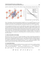
2.3 Temperature wave in linear thermo - viscoelastic material
In the pyroelectric problem (without viscous effect) through numerical calculations Yuan
and Kuang
（2008, 2010）pointed out that the term containing the inertial entropy
attenuates the temperature wave, but enhances the elastic wave. For a given material there
is a definite value of
0s


, when
00ss



 the amplitude of the elastic wave will
be increased with time. For
3
BaTio

0s


is about
13
10 s

. In the Lord－Shulman theory
critical value
0


is about
8
10 s

. In order to substantially eliminate the increasing effect of
the amplitude of the elastic wave the viscoelastic effect is considered as shown in this
section.
Using the irreversible thermodynamics (Groet, 1952; Kuang, 1999, 2002) we can assume









2

0
0
,,,
0
,,
0
12 12
,/
),
,d,
ijkljilk ijij
r
ij ijkl kl ij ij ij
ij
t
ijkl ji lk j j ijkl ji lk ij i j
t
i
ij ijkl kl i i ij j i i i
ij
CTC
Cs CT
hTd
hhTTq
  
 
  


       





       


 
 
g
gg
 
,
jj
ri
ij ijkl kl ijkl kl ij
ij ij
C

  
  

(15)
where


r
i
j


and


i
i
j

are the reversible and irreversible parts of the stress
ij

, dd
ij ij
t




.
Comparing Eqs. (9) and (10) with (15) it is found that only a term
ijkl ji lk



is added to the
rate of the complement dissipative energy in Eq. (15) . Substituting the entropy
s
and
i
T



in
Eq. (15) and

a
s
in (2) into
()
,
()
a
ii
Ts Ts r T



in Eq. (2) we still get the same equation (12).
Substituting the stress
σ in Eq. (15) into (13) we get



,,,
,
,
ijkl kl ijkl kl ij i i i ijkl k lj ijkl k lj ij j i
j
C
f
uoruCu u

f
    

   

(16)
In one dimensional problem for the isotropic material from Eq. (15) we have

0
,/YsCT

  

 

(17)

Thermodynamics – Kinetics of Dynamic Systems

6
where Y is the elastic modulus,

is a viscose coefficient,

is the temperature coefficient.
When there is no body force and body heat source, Eqs. (12) and (16) are reduced to



00

0
0
s
CTu
uYu u
   




 
  

 

 
(18)
where
,tx



   

for any function

. For a plane wave propagating along
direction x we assume






exp i , exp iuU kx t kx t
 

 


(19)
where ,
U  are the amplitudes of u and

respectively, k is the wave number and

is
the circular frequency. Substituting Eq. (19) into (18) we obtain




22
22
00
ii0
i0
s
Yk Uk
Tk U k C
  

   








(20)
In order to have nontrivial solutions for ,
U

, the coefficient determinant of Eq. (20) should
be vanished:




22
22
22
2
00
0
ii
i
0
i
s

Yk k
ak k
Tk k C
Tk k Cb
  
 
   
 






(21a)
where

i
222
i
222
00
i, ,sin
i, 1,sin
Y
T
YY YY
sTT s TT
aY re r aa Y r
brerbb r



    
    
     
   
(21b)
From Eq. (21) we get








42222
0
ii i
22
0
1212
2
i
ii i
22 2
00
i0
1
eeie

2
eeie4i
TY Y
TY
TY Y
YT
Y
YT YT
ak Cab T k Cb
kCrr T
r
Cr r T T r r e
 

 
    
  

    



   













 






(22)
where the symbol “+” is applied to the wave number
T
k of the temperature wave and the
symbol “
 ” is applied to the wave number of the viscoelastic wave
Y
k . If the temperature
wave does not couple with the elastic wave, then

is equal to zero. In this case we have









1
ii ii
22
i2 i2
2
,
TY TY
YT
YTY TY
YY TT
krCrre e Crre e
k r e k Cr e
 

 
 





(23)

Some Thermodynamic Problems in Continuum Mechanics

7
Because 0
Y


due to 0

 and 0
T

 due to
0
0
s

 , a pure viscoelastic wave or a pure
temperature waves is attenuated. The pure elastic wave does not attenuate due to 0

 .
For the general case in Eq. (22) a coupling term
22
0
i Tk


is appeared. It is known that




ii i ii i
22 22
00
Im e eie Im e eie
TY Y TY Y

YT YT
Cr r T Cr r T
   
     
 
  

It means that
Im 0
T
k  or the temperature wave is always an attenuated wave. If







2
i
ii i
22 2
00
2
ii i
22
0
Im e e i e 4i
Im e e i e
TY

TY Y
TY Y
YT YT
YT
Cr r T T r r e
Cr r T

 
 
    
  




 



(24)

we get Im 0
Y
k  or in this case the elastic wave is an attenuated wave, otherwise is
enhanced.
Introducing the viscoelastic effect in the elastic wave as shown in this section can
substantially eliminate the increasing effect of the amplitude of the elastic wave with time.
2.4 Temperature wave in thermo-electromagneto-elastic material
In this section we discuss the linear thermo-electromagneto-elastic material without
chemical reaction and viscous effect, so the electromagnetic Gibbs free energy

e
g in Eq. (1)
should keep the temperature variable. The electromagnetic Gibbs free energy
e
g and the
complement dissipative energy
e
h in this case are assumed respectively in the following
form

 
 

-
-
2
0
,, , 0
0
(,, ,) 12 12
12 12
()(),
,,,,
ee
e kl k k ijkl ji lk kij k ij ij i j i i
mm
kij k ij ij i j i i ij ij
t
eijijjj
ee mm

ijkl jikl ijlk klij kij kji kl lk kij kji kl
EH C eE EE E
eH HH H TC
hTd TT
CC C Cee ee
 
 

 


   
    

g
,
lk i
jj
i



(25)

where ,,,,,
eemm
kij kl i kij kl i
ee
 
are material constants. The constitutive equations are



+
+
0
,, ,
0
,
,/
d,
em e e
i
j
i
j
kl kl ki
j
kki
j
ki
j
ii
jj
i
j
k
j
ki
mm em
i ij j ijk jk i ij ij i i i i

t
ivi ij j iiijj
CeEeH DEe
BHe s EHCT
hTTq




  

    


(26)
Similar to derivations in sections 2.2 and 2.3 it is easy to get the governing equations:




0,
,
/
em
i
j
i
j
ii i i s i
jj

i
TEHCTTTr
     
   



(27)

Thermodynamics – Kinetics of Dynamic Systems

8



 
++
,
,,
,
,0
em
ijkl kl kij k kij k ij i i
j
ee mm
ij j kij kl i e ij j kij kl i
ii
CeEeH fu
Ee He



  



(28)
where
e

is the density of the electric charge. The boundary conditions are omitted here.
2.5 Thermal diffusion wave in linear thermoelastic material
The Gibbs equation of the classical thermodynamics with the thermal diffusion is:



,, , ,
,
, ,
:,
ii ii ii i ii
i
Ts r
q
dTscr
q
rT d c
Ts c sT c






  
 
σε σ: ε
     





gU
(29)
where

is the chemical potential, d is the flow vector of the diffusing mass, c is the
concentration. In discussion of the thermal diffusion problem we can also use the free
energy
c
sT c

σ : ε




g (Kuang, 2010), but here it is omitted. Using relations







112 1 1 1
,,,
,,,
,
ii i i i ii i i
iii
Tq Tq TqT T d T d dT



   
  

From Eq. (29) (Kuang, 2010) we get:







() ()
,
()
,, ,
,
;

0, ,
r
ri
ii
i
r
i
ii ii i i i
i
ss s Ts rTqT dT
Ts Ts Ts T T Td

   
  
  
     
   

 
(30)
where

i
Ts

is the irreversible heat rate. According to the linear irreversible thermodynamics
the irreversible forces are proportional to the irreversible flow (Kuang, 2010; Gyarmati, 1970;
De Groet, 1952), we can write the evolution equations in the following form











1
,, ,,
,
i ij i ij i i ij i ij i
TTTLTTTDTTLTT
   

 
   


(31a)
where
ij
D is the diffusing coefficients and L
ij
is the coupling coefficients. The linear
irreversible thermodynamics can only give the general form of the evolution equation, the
concrete exact formula should be given by experimental results. Considering the
experimental facts and the simplicity of the requirement for the variational formula, when
the variation of T is not too large, Eq. (31a) can also be approximated by


   
   
()
,,
,, ,,
,,
0;
,
ˆˆ ˆˆ
,
i
ii ii i i
ii
j
ii
j
ii i
j
ii
j
i
ii
j
ii
j
iii
j
ii
j
i

Ts T d
TTTLT DTLTT
TTTLT DTLTT
 
  

  
   
   
   






(31b)
Especially the coefficients
ˆˆ ˆ
,, ,,,
i
j
i
j
i
j
i
j
i
j

i
j
LD LD

in Eq. (31b) can all be considered as
symmetric constants which are adopted in following sections. Eq. (31) is the extension of the
Fourier’s law and Fick’s law.
Eq. (29) shows that in the equation of the heat flow the role of Ts

is somewhat equivalent to
c


. So analogous to the inertial entropy
()a
s we can also introduce the inertial

Some Thermodynamic Problems in Continuum Mechanics

9
concentration
()a
c and introduce a general inertial entropy theory of the thermal diffusion
problem. Eq. (29) in the general inertial entropy theory is changed to (Kuang, 2010)









 
() ()
,,
,
() () () ()
00
;
d, ; d,
a
aa
ii i ii
i
tt
aa
aa aa
sc
Ts s c c r
q
rT cc d
ss sTcc c

 
 


     

 


(32)

where
c

is the inertial concentration coefficient. Applying the irreversible thermodynamics
we can get the Gibbs free energy

g and the complement dissipative energy h

as




22
0
,, , , ,,
11
,,,,,,
00
111
(,,)
222
kl ijkl ji lk ij ij ij ij
ii ii ii ii j j j j
tt
jij iij i jijiiji
CCbba

T
hT T
TLTd LDd



      
            
        


     
   

g
(33a)
where
,,
ij
abb
are also material constants. The constitutive and evolution equations are:



0
11
,,, ,,,
00
,
/,

,
ij ij ijkl kl ij ij
ij ij ij ij
tt
i i ij j ij j i i ij j ij j
Cb
sCTacbba
hTLTdhLDd




      

   

    
         
       

g
gg
(34)
Using Eq. (34)

g in Eq. (33a) can also be rewritten as










(,,) 12 12
TT
kl ijkl ji lk ij ij ij ij
Cscb


      
gg,g
(33b)
where

T

g is the energy containing the effects of temperature and concentration.
Substituting Eq. (34) into Eq. (32) we get





0
,,
,
,,
/


;
ij ij s
ij ij s ij j ij j
i
ij ij c ji ij ji ij
TCTaT
bb a r L
bb a L D Inmedium
   
     
  

 
 







(35)
If we neglect the term in second order
,ii
d

in Eq. (29), i.e. we take
,ii
Ts r

q



and assume
that
,i
T and
,j

are not dependent each other, i.e. in Eq. (31b) we assume
1
,,
,
iijji ijj
TT D



 


, then for 0r


, Eq. (35) becomes



,0 ,

,,
/
;
ij i j s ij j
ij i j c ij ji
Tu CTa
bbu a D Inmedium










(36)

Thermodynamics – Kinetics of Dynamic Systems

10
The formulas in literatures analogous to Eq. (34) can be found, such as in Sherief, Hamza,
and Saleh’s paper (2004), where they used the Maxwell-Cattaneo formula.
The momentum equation is



,
,

ijkl k l ij ij i i
j
Cu b
f
u

 
 

(37)
The above theory is easy extended to more complex materials.
3. Physical variational principle
3.1 General theory
Usually it is considered that the first law of thermodynamics is only a principle of the
energy conservation. But we found that the first law of thermodynamics is also a physical
variational principle (Kuang, 2007, 2008a, 2008b, 2009a 2011a, 2011b). Therefore the first law
of the classical thermodynamics includes two aspects: energy conservation law and physical
variational principle:

Classical Energy conservation: d d d d =0
Classical physical variational principle : d 0
V
V
VWQ
VWQ
 






Π
U
U
(38)
where
U is the internal energy per volume, W is the work applied on the body by the
environment, Q is the heat supplied by the environment . According to Gibbs theory when
the process is only slightly deviated from the equilibrium state dQ can be substituted by
dd
V
TsV

. In practice we prefer to use the free energy g :

,d d d d
Energy Principle: d d d d 0
Ph
y
sical Variational Principle: d d 0
VV
VV
Ts s T T s
VdW sTV
VW sTV
 


   
 


 


Π
gg
g
g
UU
(39)
Here the physical variational principle is considered to be one of the fundamental physical
law, which can be used to derive governing equations in continuum mechanics and other
fields. We can also give it a simple explanation that the true displacement is one kind of the
virtual displacement and obviously it satisfies the variational principle. Other virtual
displacements cannot satisfy this variational principle, otherwise the first law is not
objective. The physical variational principle is different to the usual mathematical
variational method which is based on the known physical facts. In many problems the
variation of a variable

different with displacement
u
, should be divided into local
variation and migratory variation, i.e. the variation +
u




, where the local variation




of

is the variation duo to the change of

itself and the migratory variation
u


of

is the variation of change of

due to virtual displacements. In Eqs. (38) and (39) the new
force produced by the migratory variation
u


will enter the virtual work W

or W


as
the same as the external mechanical force. But in the following sections we shall modify Eq.
(39) or (38) to deal with this problem. The physical variational principle is inseparable with
energy conservation law, so when the expressions of energies are given we get physical
variational principle immediately. We need not to seek the variational functional as that in


Some Thermodynamic Problems in Continuum Mechanics

11
usual mathematical methods. In the following sections we show how to derive the
governing equations with the general Maxwell stress of some kind of materials by using the
physical variational principle. From this physical variational principle all of the governing
equations in the continuum mechanics and physics can be carried out and this fact can be
considered as the indirect evidence of the physical variational principle.
3.2 Physical variational principle in thermo-elasticity
In the thermo-elasticity it is usually considered that only the thermal process is irreversible,
but the elastic process is reversible. So the free energy
g and the complement dissipative
energy can be assumed as that in Eq. (9). The corresponding constitutive and evolution
equations are expressed in Eq. (10). As shown in section 3.1, the variation of the virtual
temperature

is divided into local variation



due to the variation of

itself and the
migratory variation
u


due to

u :


,
,
uu ii
u



  (40)
In previous paper (Kuang, 2011a) we showed that the migratory variation of virtual electric
and magnetic potentials will produce the Maxwell stress in electromagnetic media, which is
also shown in section 3.4 of this paper. Similarly the migratory variation
u


will also
produce the general Maxwell stress which is an external temperature stress. The effective
general Maxwell stress can be obtained by the energy principle as that in electromagnetic media.
Under assumptions that the virtual mechanical displacement
u
and the virtual temperature
()or T

satisfy their own boundary conditions ,
ii
uu






 on
u
a and
T
a respectively.
The physical variational principle using the free energy in the inertial entropy theory for the
thermo-elasticity can be expressed as:


,
()
0000
()d d 0
( ) dd dd dd dd
()
q
T
Tkk
VV
tttt
i
s
VVaV
kkk kk
Va
hV u V Q W
QrTVsV a V
W f u u dV T u da


    
          




 
   
 

   




gg
(41)
where
,
kk
f
T

and
ii
n






are the given mechanical body force, surface traction and
surface entropy flow respectively. Eq. (41) is an alternative form of Eq. (39). In Eq. (41) the
term
()
,
00
dd
tt
i
ii
sT

  



is the complement dissipative heat rate per volume
corresponding to the inner complement dissipation energy rate h

. The entropy s
includes the contribution of
()
0
d
t
i
s






. The fact that the complement dissipation energy
rate
V
hdV


in
T


and the internal irreversible complement heat rate
()
0
dd
t
i
V
sV
 




in
Q



are simultaneously included in Eq. (41) allows us to get the temperature wave
equation and the boundary condition of the heat flow from the variational principle. In
Eq. (41) there are two kinds of variational formulas. The first is

,
d
T
kk
VV
dV u V W




gg , in which the integrands contain variables themselves. The
second is
V
hdV Q





, in which the integrands contain the time derivatives of variables,
so it needs integrate with time t. This is the common feature of the irreversible process
because in the irreversible process the integral is dependent to the integral path.

Thermodynamics – Kinetics of Dynamic Systems

12

It is noted that








,0
,
,,
,
1
,
0
()(/)
d12 d
12 d 12 d
(d)
ijkl kl ij i j ij ij
VV V
ij j i ij j i
aV V
T
k k ij ij k k
VV
ij ij k k ij ij k
aV
k

t
ij i j
Va
dV C u dV C T dV
n u da u dV s dV
uV s uV
snuV s uV
hdV T n da

  

     


 
 
 

   

 
 
 



g
g
1
,,

0
[( )d]
t
ij i j
V
TdV
 


(42)
Finishing the variational calculation, we have




1
,,
0
()
11
,,
00
()
( ) [ d ] d
{ [ ( ) ]d}d dd}d 0
, 12 12
q
ij j i i
a
t

ij j i i i ij i j
Va
tt
i
ij i j s
VV
TT
ij ij ij ij ij ij ij
nT uda
fuudV T n a
sTrT s V VV
ss

  
 
  
       




  
   
   


 







ij
(43)
where
T
σ is the effective or equivalent general Maxwell stress which is the external equal
axial normal temperature stress. This general Maxwell stress is first introduced and its
rationality should be proved by experiments. Obviously
T
σ can be neglected for the case of
the small strain and small change of temperature. In Eq. (43) it is seen that
u



 is
appeared in a whole. Using


() ()
1
,, , , , ,
,
() =
ii
i
j
i

jjjjj
ii i ii
i
TT Ts T Ts T T T q
   


 

and the arbitrariness of
i
u

and


, from Eq. (43) we get



,,
1
,
;
, ; , , = ,
ij j i i s i i
kl l k i i
j
iii i nn
q

fuTs rqinmedium
nT ona T n orqq ona

 


  


  



(44)
Here
T
σ

is the external temperature body force and
T

n σ is the surface traction.
The above variational principle requests prior that displacements and the temperature
satisfy the boundary conditions, so in governing equations the following equations should
also be added

on on, ; ( ),
uT
aorTTa




uu
(45)
Eqs. (44) and (45) are the governing equations of the thermo-elasticity derived from the
physical variational principle.
3.3 Physical variational principle in thermo-diffusion theory
The electro-chemical Gibbs free energy

g and the complement dissipative energy h

are
expressed in Eq. (33) and the constitutive and evolution equations are expressed in Eq. (34).

Some Thermodynamic Problems in Continuum Mechanics

13
Under assumptions that the mechanical displacement u , the temperature

and the
chemical potential

satisfy their own boundary conditions


uu,





and



 on
u
a ,
T
a and a

respectively. When the variation of temperature is not large the physical
variational principle for the thermo-elasto-diffusive problem is






,
1
0
11
,,
00
() d 0
ddd
dd dda
dd
()
q

d
T
kk
VV
t
a
VVa
tt
ii ii ii
Va
a
Va
kkk kk
Va
hdV u V Q W
QTrdVsV a
TT V T n
cV a
W f u u dV T u da

 
  
     
 



 





 

  


 

 

  
 






ΠΦ
Φ
gg
(46)
In Eqs. (46)
,
kk
f
T



ii
n





and
ii
n





are given values. In Eq. (46) Q


is related to heat
(including the heat produced by the irreversible process in the material),


Φ is related to
the diffusion energy. Eq. (46) shows that there is no term in
V
dV



h

corresponding to the
term
1
0
dda
t
n
a
T

 




, so it should not be included in Q


and
11 1
,,
00 0
dd dda dd
tt t
ii ii ii
Va V
TVTn TV
       
 


  
 
.
It is noted that we have the following relations









,
,,
,
11
,,,,
0
d12 d
12 d
12 d
ij j i ij j i
Va V VV
T
k k ij ij ij ij k k
VV
ij ij ij ij k k
a
ij ij ij ij k

V
k
t
iij iij i i
dV n u da u dV s dV c dV
uV sc b uV
sc b nuV
sc b uV
hTTLTd



 

 
 
 

 
   
   

  
  




g
g



,,
0
t
ij i ij i
V
LT D d dV



(47)
The further derivation is fully similar to that in the thermo-elasticity. Combining Eqs. (46)
and (47) we get






,
11
,, ,,
00
11
,, ,,
00
,
,
1

0
()( )
ij j i i ij j i i i
aV VV
tt
j ij i ij i j ij i ij i
a
tt
ij i ij i ij i ij i
V
j
j
t
nT uda
f
u u dV s dV c dV
n TTLT d n LTD dda
TT LT d LT D d dV
Trd


       
      
      





 












 
 




Π
 

11
,,
0
ddd
dd dd0
qd
aa
VVV
t
ii ii

aaV
Vs Vc V
aaTTT V
  
     
 

  




(48)