basic fin math
Bạn đang xem bản rút gọn của tài liệu. Xem và tải ngay bản đầy đủ của tài liệu tại đây (486.26 KB, 106 trang )
The Basics of Financial Mathematics
Spring 2003
Richard F. Bass
Department of Mathematics
University of Connecticut
These notes are
c
2003 by Richard Bass. They may be used for personal use or
class use, but not for commercial purposes. If you find any errors, I would appreciate
hearing from you:
1
1. Introduction.
In this course we will study mathematical finance. Mathematical finance is not
about predicting the price of a stock. What it is about is figuring out the price of options
and derivatives.
The most familiar type of option is the option to buy a stock at a given price at
a given time. For example, suppose Microsoft is currently selling today at $40 p e r share.
A European call option is something I can buy that gives me the right to buy a share of
Microsoft at some future date. To make up an example, suppose I have an option that
allows me to buy a share of Microsoft for $50 in three months time, but does not compel
me to do so. If Microsoft happens to be selling at $45 in three months time, the option is
worthless. I would be silly to buy a share for $50 when I could call my broker and buy it
for $45. So I would choose not to exercise the option. On the other hand, if Microsoft is
selling for $60 three months from now, the option would be quite valuable. I could exercise
the option and buy a share for $50. I could then turn around and sell the share on the
open market for $60 and make a profit of $10 per share. Therefore this s tock option I
possess has some value. There is some chance it is worthless and some chance that it will
lead me to a profit. The basic question is: how much is the option worth today?
The huge impetus in financial derivatives was the seminal paper of Black and Scholes
in 1973. Although many researchers had studied this question, Black and Scholes gave a
definitive answer, and a great deal of research has been done since. These are not just
academic questions; today the market in financial derivatives is larger than the market
in stock securities. In other words, more money is invested in options on stocks than in
stocks themselves.
Options have been around for a long time. The earliest ones were used by manu-
facturers and food producers to hedge their risk. A farmer might agree to sell a bushel of
wheat at a fixed price six months from now rather than take a chance on the vagaries of
market prices. Similarly a steel refinery might want to lock in the price of iron ore at a
fixed price.
The sections of these notes can be grouped into five categories. The first is elemen-
tary probability. Although s ome one who has had a course in undergraduate probability
will be familiar with some of this, we will talk about a number of topics that are not usu-
ally covered in such a c ourse: σ-fields, conditional expectations, martingales. The second
category is the binomial asset pricing model. This is just about the simplest model of a
stock that one can imagine, and this will provide a case where we can see most of the major
ideas of mathematical finance, but in a very simple setting. Then we will turn to advanced
probability, that is, ideas such as Brownian motion, stochastic integrals, stochastic differ-
ential equations, Girsanov transformation. Although to do this rigorously requires measure
theory, we can still learn enough to understand and work with these concepts. We then
2
return to finance and work with the continuous model. We will derive the Black-Scholes
formula, see the Fundamental Theorem of Asset Pricing, work with equivalent martingale
measures, and the like. The fifth main category is term structure models, which means
models of interest rate behavior.
I found some unpublished notes of Steve Shreve extremely useful in preparing these
notes. I hope that he has turned them into a book and that this book is now available.
The stochastic calculus part of thes e notes is from my own book: Probabilistic Techniques
in Analysis, Springer, New York, 1995.
I would also like to thank Evarist Gin´e who pointed out a number of errors.
3
2. Review of elementary probability.
Let’s begin by recalling some of the definitions and basic concepts of elementary
probability. We will only work with discrete mo dels at first.
We start with an arbitrary set, called the probability space, which we will denote
by Ω, the capital Greek letter “omega.” We are given a class F of subsets of Ω. These are
called events. We require F to be a σ-field.
Definition 2.1. A c ollection F of subsets of Ω is called a σ-field if
(1) ∅ ∈ F,
(2) Ω ∈ F,
(3) A ∈ F implies A
c
∈ F, and
(4) A
1
, A
2
, . . . ∈ F implies both ∪
∞
i=1
A
i
∈ F and ∩
∞
i=1
A
i
∈ F.
Here A
c
= {ω ∈ Ω : ω /∈ A} denotes the complement of A. ∅ denotes the empty set, that
is, the set with no elements. We will use without special comment the usual notations of
∪ (union), ∩ (intersection), ⊂ (contained in), ∈ (is an element of).
Typically, in an elementary probability course, F will consist of all subsets of
Ω, but we will later need to distinguish be tween various σ-fields. Here is an exam-
ple. Suppose one tosses a coin two times and lets Ω denote all possible outcomes. So
Ω = {HH, HT, T H, T T }. A typical σ-field F would be the collection of all subsets of Ω.
In this case it is trivial to show that F is a σ-field, since every subset is in F. But if
we let G = {∅, Ω, {HH, HT }, {T H, T T}}, then G is also a σ-field. One has to check the
definition, but to illustrate, the event {HH, HT } is in G, so we require the complement of
that set to be in G as well. But the complement is {T H, T T} and that event is indeed in
G.
One point of view which we will explore much more fully later on is that the σ-field
tells you what events you “know.” In this example, F is the σ-field where you “know”
everything, while G is the σ-field where you “know” only the result of the first toss but not
the second. We won’t try to be precise here, but to try to add to the intuition, suppose
one knows whether an event in F has happened or not for a particular outcome. We
would then know which of the events {HH}, {HT }, {T H}, or {T T} has happened and so
would know what the two tosses of the coin showed. On the other hand, if we know which
events in G happened, we would only know whether the event {HH, HT } happened, which
means we would know that the first toss was a heads, or we would know whether the event
{T H, T T} happened, in which case we would know that the first toss was a tails. But
there is no way to tell what happened on the second toss from knowing which events in G
happened. Much more on this later.
The third basic ingredient is a probability.
4
Definition 2.2. A function P on F is a probability if it satisfies
(1) if A ∈ F, then 0 ≤ P(A) ≤ 1,
(2) P(Ω) = 1, and
(3) P(∅) = 0, and
(4) if A
1
, A
2
, . . . ∈ F are pairwise disjoint, then P(∪
∞
i=1
A
i
) =
∞
i=1
P(A
i
).
A collection of sets A
i
is pairwise disjoint if A
i
∩ A
j
= ∅ unless i = j.
There are a number of conclusions one can draw from this definition. As one
example, if A ⊂ B, then P(A) ≤ P(B) and P(A
c
) = 1 − P(A). See Note 1 at the end of
this section for a proof.
Someone who has had measure theory will realize that a σ-field is the same thing
as a σ-algebra and a probability is a measure of total mass one.
A random variable (abbreviated r.v.) is a function X from Ω to R, the reals. To
be more precise, to be a r.v. X must also be measurable, which means that {ω : X(ω) ≥
a} ∈ F for all reals a.
The notion of measurability has a simple definition but is a bit subtle. If we take
the point of view that we know all the events in G, then if Y is G-measurable, then we
know Y . Phrased another way, suppose we know whether or not the event has occurred
for each event in G. Then if Y is G-measurable, we can compute the value of Y .
Here is an example. In the example above where we tossed a coin two times, let X
be the number of heads in the two tosses. Then X is F measurable but not G measurable.
To see this, let us consider A
a
= {ω ∈ Ω : X(ω) ≥ a}. This event will equal
Ω if a ≤ 0;
{HH, HT, T H} if 0 < a ≤ 1;
{HH} if 1 < a ≤ 2;
∅ if 2 < a.
For example, if a =
3
2
, then the event where the number of heads is
3
2
or greater is the
event where we had two heads, namely, {HH}. Now observe that for each a the event A
a
is in F because F contains all subsets of Ω. Therefore X is measurable with respect to F.
However it is not true that A
a
is in G for every value of a – take a =
3
2
as just one example
– the subset {HH} is not in G. So X is not measurable with respect to the σ-field G.
A discrete r.v. is one where P(ω : X(ω) = a) = 0 for all but countably many a’s,
say, a
1
, a
2
, . . ., and
i
P(ω : X(ω) = a
i
) = 1. In defining sets one usually omits the ω;
thus (X = x) means the same as {ω : X(ω) = x}.
In the discrete cas e, to check measurability with respect to a σ-field F, it is enough
that (X = a) ∈ F for all reals a. The reason for this is that if x
1
, x
2
, . . . are the values of
5
x for which P(X = x) = 0, then we can write (X ≥ a) = ∪
x
i
≥a
(X = x
i
) and we have a
countable union. So if (X = x
i
) ∈ F, then (X ≥ a) ∈ F.
Given a discrete r.v. X, the expec tation or mean is defined by
E X =
x
xP(X = x)
provided the sum converges. If X only takes finitely many values, then this is a finite sum
and of course it will converge. This is the situation that we will consider for quite some
time. However, if X can take an infinite number of values (but countable), convergence
needs to be checked. For example, if P(X = 2
n
) = 2
−n
for n = 1, 2, . . ., then E X =
∞
n=1
2
n
· 2
−n
= ∞.
There is an alternate definition of expectation which is equivalent in the discrete
setting. Set
E X =
ω∈Ω
X(ω)P({ω}).
To see that this is the same, look at Note 2 at the end of the section. The advantage of the
second definition is that some properties of expectation, s uch as E (X + Y ) = E X + E Y ,
are immediate, while with the first definition they require quite a bit of proof.
We say two events A and B are independent if P(A ∩B) = P(A)P(B). Two random
variables X and Y are independent if P(X ∈ A, Y ∈ B) = P(X ∈ A)P(X ∈ B) for all A
and B that are subsets of the reals. The comma in the expression P(X ∈ A, Y ∈ B) means
“and.” Thus
P(X ∈ A, Y ∈ B) = P((X ∈ A) ∩ (Y ∈ B)).
The extension of the definition of independence to the case of more than two events or
random variables is not surprising: A
1
, . . . , A
n
are independent if
P(A
i
1
∩ ···∩A
i
j
) = P(A
i
1
) ···P(A
i
j
)
whenever {i
1
, . . . , i
j
} is a subset of {1, . . . , n}.
A common misconception is that an event is independent of itself. If A is an event
that is independent of itself, then
P(A) = P(A ∩A) = P(A)P(A) = (P(A))
2
.
The only finite solutions to the equation x = x
2
are x = 0 and x = 1, so an event is
independent of itself only if it has probability 0 or 1.
Two σ-fields F and G are independent if A and B are independent whenever A ∈ F
and B ∈ G. A r.v. X and a σ-field G are independent if P((X ∈ A) ∩B) = P(X ∈ A)P(B)
whenever A is a subset of the reals and B ∈ G.
6
As an example, suppose we toss a coin two times and we define the σ-fields G
1
=
{∅, Ω, {HH, HT }, {T H, T T}} and G
2
= {∅, Ω, {HH, T H}, {HT, T T }}. Then G
1
and G
2
are
independent if P(HH) = P(HT ) = P(T H) = P(T T) =
1
4
. (Here we are writing P(HH)
when a more accurate way would be to write P({HH}).) An easy way to understand this
is that if we look at an event in G
1
that is not ∅ or Ω, then that is the event that the first
toss is a heads or it is the event that the first toss is a tails. Similarly, a set other than ∅
or Ω in G
2
will be the event that the second toss is a heads or that the second toss is a
tails.
If two r.v.s X and Y are independent, we have the multiplication theorem, which
says that E (XY ) = (E X)(E Y ) provided all the expectations are finite. See Note 3 for a
proof.
Suppose X
1
, . . . , X
n
are n independent r.v.s, such that for each one P(X
i
= 1) = p,
P(X
i
= 0) = 1 − p, where p ∈ [0, 1]. The random variable S
n
=
n
i=1
X
i
is called a
binomial r.v., and represents, for example, the number of successes in n trials, where the
probability of a success is p. An important result in probability is that
P(S
n
= k) =
n!
k!(n −k)!
p
k
(1 −p)
n−k
.
The variance of a random variable is
Var X = E [(X −E X)
2
].
This is also equal to
E [X
2
] −(E X)
2
.
It is an easy consequence of the multiplication theorem that if X and Y are indepe ndent,
Var (X + Y ) = Var X + Var Y.
The expression E [X
2
] is sometimes called the second moment of X.
We close this section with a definition of conditional probability. The probability
of A given B, written P(A | B) is defined by
P(A ∩B)
P(B)
,
provided P(B) = 0. The conditional expectation of X given B is defined to be
E [X; B]
P(B)
,
7
provided P(B) = 0. The notation E [X; B] means E [X1
B
], where 1
B
(ω) is 1 if ω ∈ B and
0 otherwise. Another way of writing E [X; B] is
E [X; B] =
ω∈B
X(ω)P({ω}).
(We will use the notation E [X; B] frequently.)
Note 1. Suppose we have two disjoint sets C and D. Let A
1
= C, A
2
= D, and A
i
= ∅ for
i ≥ 3. Then the A
i
are pairwise disjoint and
P(C ∪ D) = P(∪
∞
i=1
A
i
) =
∞
i=1
P(A
i
) = P(C) + P(D) (2.1)
by Definition 2.2(3) and (4). Therefore Definition 2.2(4) holds when there are only two sets
instead of infinitely many, and a similar argument shows the same is true when there are an
arbitrary (but finite) number of sets.
Now suppose A ⊂ B. Let C = A and D = B − A, where B − A is defined to be
B ∩A
c
(this is frequently written B \ A as well). Then C and D are disjoint, and by (2.1)
P(B) = P(C ∪ D) = P(C) + P(D) ≥ P(C) = P(A).
The other equality we mentioned is proved by letting C = A and D = A
c
. Then C and
D are disjoint, and
1 = P(Ω) = P(C ∪ D) = P(C) + P(D) = P(A) + P(A
c
).
Solving for P(A
c
), we have
P(A
c
) = 1 −P(A).
Note 2. Let us show the two definitions of expectation are the same (in the discrete case).
Starting with the first definition we have
E X =
x
xP(X = x)
=
x
x
{ω∈Ω:X(ω)=x}
P({ω})
=
x
{ω∈Ω:X(ω)=x}
X(ω)P({ω})
=
ω∈Ω
X(ω)P({ω}),
8
and we end up with the second definition.
Note 3. Suppose X can takes the values x
1
, x
2
, . . . and Y can take the values y
1
, y
2
, . .
Let A
i
= {ω : X(ω) = x
i
} and B
j
= {ω : Y (ω) = y
j
}. Then
X =
i
x
i
1
A
i
, Y =
j
y
j
1
B
j
,
and so
XY =
i
j
x
i
y
i
1
A
i
1
B
j
.
Since 1
A
i
1
B
j
= 1
A
i
∩B
j
, it follows that
E [XY ] =
i
j
x
i
y
j
P(A
i
∩ B
j
),
assuming the double sum converges. Since X and Y are independent, A
i
= (X = x
i
) is
independent of B
j
= (Y = y
j
) and so
E [XY ] =
i
j
x
i
y
j
P(A
i
)P(B
j
)
=
i
x
i
P(A
i
)
j
y
j
P(B
j
)
=
i
x
i
P(A
i
)E Y
= (E X)(E Y ).
9
3. Conditional expectation.
Suppose we have 200 men and 100 women, 70 of the men are smokers, and 50 of
the women are smokers. If a person is chosen at random, then the conditional probability
that the person is a smoker given that it is a man is 70 divided by 200, or 35%, while the
conditional probability the person is a smoker given that it is a women is 50 divided by
100, or 50%. We will want to be able to encompass both facts in a single entity.
The way to do that is to make conditional probability a random variable rather
than a number. To reiterate, we will make conditional probabilities random. Let M, W be
man, woman, respectively, and S, S
c
smoker and nonsmoker, respectively. We have
P(S | M) = .35, P(S | W ) = .50.
We introduce the random variable
(.35)1
M
+ (.50)1
W
and use that for our conditional probability. So on the set M its value is .35 and on the
set W its value is .50.
We need to give this random variable a name, so what we do is let G be the σ-field
consisting of {∅, Ω, M, W } and denote this random variable P(S | G). Thus we are going
to talk about the conditional probability of an event given a σ-field.
What is the precise definition?
Definition 3.1. Suppose there exist finitely (or countably) many sets B
1
, B
2
, . . ., all hav-
ing positive probability, such that they are pairwise disjoint, Ω is equal to their union, and
G is the σ-field one obtains by taking all finite or countable unions of the B
i
. Then the
conditional probability of A given G is
P(A | G) =
i
P(A ∩B
i
)
P(B
i
)
1
B
i
(ω).
In short, on the set B
i
the conditional probability is equal to P(A | B
i
).
Not every σ-field can be so represented, so this definition will need to be extended
when we get to continuous models. σ-fields that can be represented as in Definition 3.B are
called finitely (or countably) generated and are said to be generated by the sets B
1
, B
2
, . .
Let’s look at another example. Suppose Ω consists of the possible results when we
toss a coin three times: HHH, HHT, etc. Let F
3
denote all subsets of Ω. Let F
1
consist of
the sets ∅, Ω, {HHH, HHT, HT H, HT T }, and {T HH, T HT, T T H, T TT }. So F
1
consists
of those events that can be determined by knowing the result of the first toss. We want to
let F
2
denote those events that can be determined by knowing the first two tosses. This will
10
include the sets ∅, Ω, {HHH, HHT }, {HT H, HT T}, {T HH, T HT }, {T T H, T TT }. This is
not enough to make F
2
a σ-field, so we add to F
2
all sets that can be obtained by taking
unions of these sets.
Suppose we tossed the coin independently and suppose that it was fair. Let us
calculate P(A | F
1
), P(A | F
2
), and P(A | F
3
) when A is the event {HHH}. First
the conditional probability given F
1
. Let C
1
= {HHH, HHT, HT H, HT T } and C
2
=
{T HH, T HT, T T H, T T T }. On the set C
1
the conditional probability is P(A∩C
1
)/P(C
1
) =
P(HHH)/P(C
1
) =
1
8
/
1
2
=
1
4
. On the set C
2
the conditional probability is P(A∩C
2
)/P(C
2
)
= P(∅)/P(C
2
) = 0. Therefore P(A | F
1
) = (.25)1
C
1
. This is plausible – the probability of
getting three heads given the first toss is
1
4
if the first toss is a heads and 0 otherwise.
Next let us calculate P(A | F
2
). Le t D
1
= {HHH, HHT }, D
2
= {HT H, HT T }, D
3
= {T HH, T HT }, D
4
= {T T H, T T T }. So F
2
is the σ-field consisting of all possible unions
of some of the D
i
’s. P(A | D
1
) = P(HHH)/P(D
1
) =
1
8
/
1
4
=
1
2
. Also, as above, P(A |
D
i
) = 0 for i = 2, 3, 4. So P(A | F
2
) = (.50)1
D
1
. This is again plausible – the probability
of getting three heads given the first two tosses is
1
2
if the first two tosses were heads and
0 otherwise.
What about conditional expectation? Recall E [X; B
i
] = E [X1
B
i
] and also that
E [1
B
] = 1 ·P(1
B
= 1) + 0 · P(1
B
= 0) = P(B). Given a random variable X, we define
E [X | G] =
i
E [X; B
i
]
P(B
i
)
1
B
i
.
This is the obvious definition, and it agrees with what we had before because E [1
A
| G]
should be equal to P(A | G).
We now turn to some properties of conditional expectation. Some of the following
propositions may seem a bit technical. In fact, they are! However, these properties are
crucial to what follows and there is no choice but to master them.
Proposition 3.2. E [X | G] is G measurable, that is, if Y = E [X | G], then (Y > a) is a
set in G for each real a.
Proof. By the definition,
Y = E [X | G] =
i
E [X; B
i
]
P(B
i
)
1
B
i
=
i
b
i
1
B
i
if we set b
i
= E [X; B
i
]/P(B
i
). The set (Y ≥ a) is a union of some of the B
i
, namely, those
B
i
for which b
i
≥ a. But the union of any collection of the B
i
is in G.
An example might help. Suppose
Y = 2 ·1
B
1
+ 3 ·1
B
2
+ 6 ·1
B
3
+ 4 ·1
B
4
and a = 3.5. Then (Y ≥ a) = B
3
∪ B
4
, which is in G.
11
Proposition 3.3. If C ∈ G and Y = E [X | G], then E [Y ; C] = E [X; C].
Proof. Since Y =
E [X; B
i
]
P(B
i
)
1
B
i
and the B
i
are disjoint, then
E [Y ; B
j
] =
E [X; B
j
]
P(B
j
)
E 1
B
j
= E [X; B
j
].
Now if C = B
j
1
∪···∪B
j
n
∪···, summing the above over the j
k
gives E [Y ; C] = E [X; C].
Let us look at the above example for this proposition, and let us do the case where
C = B
2
. Note 1
B
2
1
B
2
= 1
B
2
because the product is 1 ·1 = 1 if ω is in B
2
and 0 otherwise.
On the other hand, it is not poss ible for an ω to be in more than one of the B
i
, so
1
B
2
1
B
i
= 0 if i = 2. Multiplying Y in the above example by 1
B
2
, we see that
E [Y ; C] = E [Y ; B
2
] = E [Y 1
B
2
] = E [3 ·1
B
2
]
= 3E [1
B
2
] = 3P(B
2
).
However the number 3 is not just any number; it is E [X; B
2
]/P(B
2
). So
3P(B
2
) =
E [X; B
2
]
P(B
2
)
P(B
2
) = E [X; B
2
] = E [X; C],
just as we wanted. If C = B
1
∪ B
4
, for example, we then write
E [X; C] = E [X1
C
] = E [X(1
B
2
+ 1
B
4
)]
= E [X1
B
2
] + E [X1
B
4
] = E [X; B
2
] + E [X; B
4
].
By the first part, this equals E [Y ; B
2
]+E [Y ; B
4
], and we undo the above string of equalities
but with Y instead of X to see that this is E [Y ; C].
If a r.v. Y is G measurable, then for any a we have (Y = a) ∈ G which means that
(Y = a) is the union of one or more of the B
i
. Since the B
i
are disjoint, it follows that Y
must be constant on each B
i
.
Again let us look at an example. Suppose Z takes only the values 1, 3, 4, 7. Let
D
1
= (Z = 1), D
2
= (Z = 3), D
3
= (Z = 4), D
4
= (Z = 7). Note that we can write
Z = 1 · 1
D
1
+ 3 ·1
D
2
+ 4 ·1
D
3
+ 7 ·1
D
4
.
To see this, if ω ∈ D
2
, for example, the right hand side will be 0 +3·1+0+ 0, which agrees
with Z(ω). Now if Z is G measurable, then (Z ≥ a) ∈ G for e ach a. Take a = 7, and we
see D
4
∈ G. Take a = 4 and we see D
3
∪ D
4
∈ G. Taking a = 3 shows D
2
∪ D
3
∪ D
4
∈ G.
12
Now D
3
= (D
3
∪D
4
) ∩D
c
4
, so since G is a σ-field, D
3
∈ G. Similarly D
2
, D
1
∈ G. Because
sets in G are unions of the B
i
’s, we must have Z constant on the B
i
’s. For example, if it
so happened that D
1
= B
1
, D
2
= B
2
∪ B
4
, D
3
= B
3
∪ B
6
∪ B
7
, and D
4
= B
5
, then
Z = 1 · 1
B
1
+ 3 ·1
B
2
+ 4 ·1
B
3
+ 3 ·1
B
4
+ 7 ·1
B
5
+ +4 ·1
B
6
+ 4 ·1
B
7
.
We still restrict ourselves to the discrete case. In this context, the properties given
in Propositions 3.2 and 3.3 uniquely determine E [X | G].
Proposition 3.4. Suppose Z is G measurable and E [Z; C] = E [X; C] whenever C ∈ G.
Then Z = E [X | G].
Proof. Since Z is G measurable, then Z must be constant on each B
i
. Let the value of Z
on B
i
be z
i
. So Z =
i
z
i
1
B
i
. Then
z
i
P(B
i
) = E [Z; B
i
] = E [X; B
i
],
or z
i
= E [X; B
i
]/P(B
i
) as required.
The following propositions contain the main facts about this new definition of con-
ditional expectation that we will need.
Proposition 3.5. (1) If X
1
≥ X
2
, then E [X
1
| G] ≥ E [X
2
| G].
(2) E [aX
1
+ bX
2
| G] = aE [X
1
| G] + bE [X
2
| G].
(3) If X is G measurable, then E [X | G] = X.
(4) E [E [X | G]] = E X.
(5) If X is independent of G, then E [X | G] = E X.
We will prove Proposition 3.5 in Note 1 at the end of the section. At this point it
is more fruitful to understand what the proposition says.
We will see in Proposition 3.8 below that we may think of E [X | G] as the best
prediction of X given G. Accepting this for the moment, we can give an interpretation of
(1)-(5). (1) says that if X
1
is larger than X
2
, then the predicted value of X
1
should be
larger than the predicted value of X
2
. (2) says that the predicted value of X
1
+ X
2
should
be the sum of the predicted values. (3) says that if we know G and X is G measurable,
then we know X and our best prediction of X is X itself. (4) says that the average of the
predicted value of X should be the average value of X. (5) says that if knowing G gives us
no additional information on X, then the be st prediction for the value of X is just E X.
Proposition 3.6. If Z is G measurable, then E [XZ | G] = ZE [X | G].
We again defer the proof, this time to Note 2.
Proposition 3.6 says that as far as conditional expectations with respect to a σ-
field G go, G-measurable random variables act like constants: they can be taken inside or
outside the conditional expectation at will.
13
Proposition 3.7. If H ⊂ G ⊂ F, then
E [E [X | H] | G] = E [X | H] = E [E [X | G] | H].
Proof. E [X | H] is H measurable, hence G measurable, since H ⊂ G. The left hand
equality now follows by Proposition 3.5(3). To get the right hand equality, let W be the
right hand expression. It is H measurable, and if C ∈ H ⊂ G, then
E [W ; C] = E [E [X | G]; C] = E [X; C]
as required.
In words, if we are predicting a prediction of X given limited information, this is
the same as a single prediction given the least amount of information.
Let us verify that conditional expectation may be viewed as the best predictor of
a random variable given a σ-field. If X is a r.v., a predictor Z is just another random
variable, and the goodness of the prediction will be measured by E [(X − Z)
2
], which is
known as the mean square error.
Proposition 3.8. If X is a r.v., the best predictor among the collection of G-measurable
random variables is Y = E [X | G].
Proof. Let Z be any G-measurable random variable. We compute, using Proposition
3.5(3) and Proposition 3.6,
E [(X −Z)
2
| G] = E [X
2
| G] − 2E [XZ | G] + E [Z
2
| G]
= E [X
2
| G] − 2ZE [X | G] + Z
2
= E [X
2
| G] − 2ZY + Z
2
= E [X
2
| G] − Y
2
+ (Y − Z)
2
= E [X
2
| G] − 2Y E [X | G] + Y
2
+ (Y − Z)
2
= E [X
2
| G] − 2E [XY | G] + E [Y
2
| G] + (Y − Z)
2
= E [(X − Y )
2
| G] + (Y − Z)
2
.
We also used the fact that Y is G measurable. Taking expectations and using Proposition
3.5(4),
E [(X −Z)
2
] = E [(X − Y )
2
] + E [(Y − Z)
2
].
The right hand side is bigger than or equal to E [(X −Y )
2
] b ec ause (Y −Z)
2
≥ 0. So the
error in predicting X by Z is larger than the error in predicting X by Y , and will be equal
if and only if Z = Y . So Y is the best predictor.
14
There is one more interpretation of conditional expectation that may be useful. The
collection of all random variables is a linear space, and the collection of all G-measurable
random variables is clearly a subspace. Given X, the conditional expectation Y = E [X | G]
is equal to the projection of X onto the subspace of G-m eas urable random variables. To
see this, we write X = Y + (X −Y ), and what we have to check is that the inner product
of Y and X − Y is 0, that is, Y and X − Y are orthogonal. In this context, the inner
product of X
1
and X
2
is defined to be E [X
1
X
2
], so we must show E [Y (X −Y )] = 0. Note
E [Y (X − Y ) | G] = Y E [X −Y | G] = Y (E [X | G] −Y ) = Y (Y − Y ) = 0.
Taking expectations,
E [Y (X − Y )] = E [E [Y (X −Y ) | G] ] = 0,
just as we wished.
If Y is a discrete random variable, that is, it takes only countably many values
y
1
, y
2
, . . ., we let B
i
= (Y = y
i
). These will be disjoint sets whose union is Ω. If σ(Y )
is the collection of all unions of the B
i
, then σ(Y ) is a σ-field, and is called the σ-field
generated by Y . It is easy to see that this is the smallest σ-field with respect to which Y
is measurable. We write E [X | Y ] for E [X | σ(Y )].
Note 1. We prove Proposition 3.5. (1) and (2) are immediate from the definition. To prove
(3), note that if Z = X, then Z is G measurable and E [X; C] = E [Z; C] for any C ∈ G; this
is trivial. By Proposition 3.4 it follows that Z = E [X | G];this proves (3). To prove (4), if we
let C = Ω and Y = E [X | G], then E Y = E [Y ; C] = E [X; C] = E X.
Last is (5). Let Z = E X. Z is constant, so clearly G measurable. By the in-
dependence, if C ∈ G, then E [X; C] = E [X1
C
] = (E X)(E 1
C
) = (E X)(P(C)). But
E [Z; C] = (E X)(P(C)) since Z is constant. By Proposition 3.4 we see Z = E [X | G].
Note 2. We prove Proposition 3.6. Note that ZE [X | G] is G measurable, so by Proposition
3.4 we need to show its ex pectation over sets C in G is the same as that of XZ. As in the
proof of Proposition 3.3, it suffices to consider only the case when C is one of the B
i
. Now Z
is G measurable, hence it is constant on B
i
; let its value be z
i
. Then
E [ZE [X | G]; B
i
] = E [z
i
E [X | G]; B
i
] = z
i
E [E [X | G]; B
i
] = z
i
E [X; B
i
] = E [XZ; B
i
]
as desired.
15
4. Martingales.
Suppose we have a sequence of σ-fields F
1
⊂ F
2
⊂ F
3
···. An example would be
repeatedly tossing a coin and letting F
k
be the sets that can be determined by the first
k tosses. Another example is to let F
k
be the events that are determined by the values
of a stock at times 1 through k. A third example is to let X
1
, X
2
, . . . be a sequence of
random variables and let F
k
be the σ-field generated by X
1
, . . . , X
k
, the smallest σ-field
with respect to which X
1
, . . . , X
k
are measurable.
Definition 4.1. A r.v. X is integrable if E |X| < ∞. Given an increasing sequence of
σ-fields F
n
, a sequence of r.v.’s X
n
is adapted if X
n
is F
n
measurable for each n.
Definition 4.2. A m artingale M
n
is a sequence of random variables such that
(1) M
n
is integrable for all n,
(2) M
n
is adapted to F
n
, and
(3) for all n
E [M
n+1
| F
n
] = M
n
. (4.1)
Usually (1) and (2) are easy to check, and it is (3) that is the crucial property. If
we have (1) and (2), but instead of (3) we have
(3) for all n
E [M
n+1
| F
n
] ≥ M
n
,
then we say M
n
is a submartingale. If we have (1) and (2), but instead of (3) we have
(3) for all n
E [M
n+1
| F
n
] ≤ M
n
,
then we say M
n
is a supermartingale.
Submartingales tends to increase and supermartingales tend to decrease. The
nomenclature may seem like it goes the wrong way; Doob defined these terms by anal-
ogy with the notions of subharmonic and superharmonic functions in analysis. (Actually,
it is more than an analogy: we won’t explore this, but it turns out that the composition
of a subharmonic function with Brownian motion yields a submartingale, and similarly for
superharmonic functions.)
Note that the definition of martingale depends on the collection of σ-fields. When
it is needed for clarity, one can say that (M
n
, F
n
) is a martingale. To define conditional
expectation, one needs a probability, so a martingale depends on the probability as well.
When we need to, we will say that M
n
is a martingale with respect to the probability P.
This is an issue when there is more than one probability around.
We will see that martingales are ubiquitous in financial math. For example, security
prices and one’s wealth will turn out to be examples of martingales.
16
The word “martingale” is also used for the piece of a horse’s bridle that runs from
the horse’s head to its chest. It keeps the horse from raising its head too high. It turns out
that martingales in probability cannot get too large. The word also refers to a gambling
system. I did some searching on the Internet, and there seems to be no consensus on the
derivation of the term.
Here is an example of a martingale. Let X
1
, X
2
, . . . be a sequence of indepe ndent
r.v.’s with mean 0 that are independent. (Saying a r.v. X
i
has mean 0 is the same as
saying E X
i
= 0; this pres uppose s that E |X
1
| is finite.) Set F
n
= σ(X
1
, . . . , X
n
), the
σ-field generated by X
1
, . . . , X
n
. Let M
n
=
n
i=1
X
i
. Definition 4.2(2) is easy to see.
Since E |M
n
| ≤
n
i=1
E |X
i
|, Definition 4.2(1) also holds. We now check
E [M
n+1
| F
n
] = X
1
+ ···+ X
n
+ E [X
n+1
| F
n
] = M
n
+ E X
n+1
= M
n
,
where we used the independence.
Another example: suppose in the above that the X
k
all have variance 1, and let
M
n
= S
2
n
−n, where S
n
=
n
i=1
X
i
. Again (1) and (2) of Definition 4.2 are easy to check.
We compute
E [M
n+1
| F
n
] = E [S
2
n
+ 2X
n+1
S
n
+ X
2
n+1
| F
n
] −(n + 1).
We have E [S
2
n
| F
n
] = S
2
n
since S
n
is F
n
measurable.
E [2X
n+1
S
n
| F
n
] = 2S
n
E [X
n+1
| F
n
] = 2S
n
E X
n+1
= 0.
And E [X
2
n+1
| F
n
] = E X
2
n+1
= 1. Substituting, we obtain E [M
n+1
| F
n
] = M
n
, or M
n
is
a martingale.
A third example: Suppose you start with a dollar and you are tossing a fair coin
independently. If it turns up heads you double your fortune, tails you go broke. This is
“double or nothing.” Let M
n
be your fortune at time n. To formalize this, let X
1
, X
2
, . . .
be independent r.v.’s that are equal to 2 with probability
1
2
and 0 with probability
1
2
. Then
M
n
= X
1
···X
n
. Let F
n
be the σ-field generated by X
1
, . . . , X
n
. Note 0 ≤ M
n
≤ 2
n
, and
so Definition 4.2(1) is satisfied, while (2) is easy. To compute the conditional expectation,
note E X
n+1
= 1. Then
E [M
n+1
| F
n
] = M
n
E [X
n+1
| F
n
] = M
n
E X
n+1
= M
n
,
using the independence.
Before we give our fourth example, let us observe that
|E [X | F]| ≤ E [|X| | F]. (4.2)
To see this, we have −|X| ≤ X ≤ |X|, so −E [|X| | F] ≤ E [X | F] ≤ E [|X| | F]. Since
E [|X| | F] is nonnegative, (4.2) follows.
Our fourth example will be used many times, so we state it as a proposition.
17
Proposition 4.3. Let F
1
, F
2
, . . . be given and let X be a fixed r.v. with E |X| < ∞. Let
M
n
= E [X | F
n
]. Then M
n
is a martingale.
Proof. Definition 4.2(2) is clear, while
E |M
n
| ≤ E [E [|X| | F
n
]] = E |X| < ∞
by (4.2); this shows Definition 4.2(1). We have
E [M
n+1
| F
n
] = E [E [X | F
n+1
] | F
n
] = E [X | F
n
] = M
n
.
18
5. Properties of martingales.
When it comes to discussing American options, we will need the concept of stopping
times. A mapping τ from Ω into the nonnegative integers is a stopping time if (τ = k) ∈ F
k
for each k.
An example is τ = min{k : S
k
≥ A}. This is a stopping time because (τ = k) =
(S
1
, . . . , S
k−1
< A, S
k
≥ A) ∈ F
k
. We can think of a stopping time as the first time
something happens. σ = max{k : S
k
≥ A}, the last time, is not a stopping time. (We will
use the convention that the minimum of an empty set is +∞; so, for example, with the
above definition of τ, on the event that S
k
is never in A, we have τ = ∞.
Here is an intuitive description of a stopping time. If I tell you to drive to the city
limits and then drive until you come to the second stop light after that, you know when
you get there that you have arrived; you don’t need to have been there before or to look
ahead. But if I tell you to drive until you come to the second stop light before the city
limits, either you must have been there before or else you have to go past where you are
supposed to stop, continue on to the city limits, and then turn around and come back two
stop lights. You don’t know when you first get to the second stop light before the city
limits that you get to stop there. The first set of instructions forms a stopping time, the
second set does not.
Note (τ ≤ k) = ∪
k
j=0
(τ = j). Since (τ = j) ∈ F
j
⊂ F
k
, then the event (τ ≤ k) ∈ F
k
for all k. Conversely, if τ is a r.v. with (τ ≤ k) ∈ F
k
for all k, then
(τ = k) = (τ ≤ k) − (τ ≤ k −1).
Since (τ ≤ k) ∈ F
k
and (τ ≤ k − 1) ∈ F
k−1
⊂ F
k
, then (τ = k) ∈ F
k
, and such a τ must
be a stopping time.
Our first result is Jensen’s inequality.
Proposition 5.1. If g is convex, then
g(E [X | G]) ≤ E [g(X) | G]
provided all the expectations exist.
For ordinary expectations rather than conditional expectations, this is still true.
That is, if g is convex and the expectations exist, then
g(E X) ≤ E [g(X)].
We already know some special cases of this: when g(x) = |x|, this says |E X| ≤ E |X|;
when g(x) = x
2
, this says (E X)
2
≤ E X
2
, which we know because E X
2
− (E X)
2
=
E (X −E X)
2
≥ 0.
19
For Proposition 5.1 as well as many of the following propositions, the statement of
the result is more important than the proof, and we relegate the proof to Note 1 below.
One reason we want Jensen’s inequality is to show that a convex function applied
to a martingale yields a submartingale.
Proposition 5.2. If M
n
is a martingale and g is convex, then g(M
n
) is a submartingale,
provided all the expectations exist.
Proof. By Jensen’s inequality,
E [g(M
n+1
) | F
n
] ≥ g(E [M
n+1
| F
n
]) = g(M
n
).
If M
n
is a martingale, then E M
n
= E [E [M
n+1
| F
n
]] = E M
n+1
. So E M
0
=
E M
1
= ··· = E M
n
. Doob’s optional stopping theorem says the same thing holds when
fixed times n are replaced by stopping times.
Theorem 5.3. Suppose K is a positive integer, N is a stopping time such that N ≤ K
a.s., and M
n
is a martingale. Then
E M
N
= E M
K
.
Here, to evaluate M
N
, one first finds N(ω) and then evaluates M
·
(ω) for that value of N.
Proof. We have
E M
N
=
K
k=0
E [M
N
; N = k].
If we show that the k-th summand is E [M
n
; N = k], then the sum will be
K
k=0
E [M
n
; N = k] = E M
n
as desired. We have
E [M
N
; N = k] = E [M
k
; N = k]
by the definition of M
N
. Now (N = k) is in F
k
, so by Proposition 2.2 and the fact that
M
k
= E [M
k+1
| F
k
],
E [M
k
; N = k] = E [M
k+1
; N = k].
We have (N = k) ∈ F
k
⊂ F
k+1
. Since M
k+1
= E [M
k+2
| F
k+1
], Proposition 2.2 tells us
that
E [M
k+1
; N = k] = E [M
k+2
; N = k].
20
We continue, using (N = k) ∈ F
k
⊂ F
k+1
⊂ F
k+2
, and we obtain
E [M
N
; N = k] = E [M
k
; N = k] = E [M
k+1
; N = k] = ··· = E [M
n
; N = k].
If we change the equalities in the above to inequalities, the same result holds for sub-
martingales.
As a corollary we have two of Doob’s inequalities:
Theorem 5.4. If M
n
is a nonnegative submartingale,
(a) P(max
k≤n
M
k
≥ λ) ≤
1
λ
E M
n
.
(b) E (max
k≤n
M
2
k
) ≤ 4E M
2
n
.
For the proof, see Note 2 below.
Note 1. We prove Proposition 5.1. If g is convex, then the graph of g lies above all the
tangent lines. Even if g does not have a derivative at x
0
, there is a line passing through x
0
which lies beneath the graph of g. So for each x
0
there exists c(x
0
) such that
g(x) ≥ g(x
0
) + c(x
0
)(x −x
0
).
Apply this with x = X(ω) and x
0
= E [X | G](ω). We then have
g(X) ≥ g(E [X | G]) + c(E [X | G])(X −E [X | G]).
If g is differentiable, we let c(x
0
) = g
(x
0
). In the case where g is not differentiable, then we
choose c to be the left hand uppe r derivate, for example. (For those who are not familiar with
derivates, this is essentially the left hand derivative.) One can check that if c is so chosen,
then c(E [X | G]) is G measurable.
Now take the conditional expectation with respect to G. The first term on the right is
G measurable, so remains the same. The second term on the right is equal to
c(E [X | G])E [X −E [X | G] | G] = 0.
Note 2. We prove Theorem 5.4. Set M
n+1
= M
n
. It is easy to see that the sequence
M
1
, M
2
, . . . , M
n+1
is also a submartingale. Let N = min{k : M
k
≥ λ} ∧ (n + 1), the first
time that M
k
is greater than or equal to λ, where a ∧ b = min(a, b). Then
P(max
k≤n
M
k
≥ λ) = P(N ≤ n)
21
and if N ≤ n, then M
N
≥ λ. Now
P(max
k≤n
M
k
≥ λ) = E [1
(N≤n)
] ≤ E
M
N
λ
; N ≤ n
(5.1)
=
1
λ
E [M
N∧n
; N ≤ n] ≤
1
λ
E M
N∧n
.
Finally, since M
n
is a submartingale, E M
N∧n
≤ E M
n
.
We now lo ok at (b). Let us write M
∗
for max
k≤n
M
k
. If E M
2
n
= ∞, there is nothing
to prove. If it is finite, then by Jensen’s inequality, we have
E M
2
k
= E [E [M
n
| F
k
]
2
] ≤ E [E [M
2
n
| F
k
] ] = E M
2
n
< ∞
for k ≤ n. Then
E (M
∗
)
2
= E [ max
1≤k≤n
M
2
k
] ≤ E
n
k=1
M
2
k
< ∞.
We have
E [M
N∧n
; N ≤ n] =
∞
k=0
E [M
k∧n
; N = k].
Arguing as in the proof of Theorem 5.3,
E [M
k∧n
; N = k] ≤ E [M
n
; N = k],
and so
E [M
N∧n
; N ≤ n] ≤
∞
k=0
E [M
n
; N = k] = E [M
n
; N ≤ n].
The last expression is at most E [M
n
; M
∗
≥ λ]. If we multiply (5.1) by 2λ and integrate over
λ from 0 to ∞, we obtain
∞
0
2λP(M
∗
≥ λ)dλ ≤ 2
∞
0
E [M
n
: M
∗
≥ λ]
= 2E
∞
0
M
n
1
(M
∗
≥λ)
dλ
= 2E
M
n
M
∗
0
dλ
= 2E [M
n
M
∗
].
Using Cauchy-Schwarz, this is bounded by
2(E M
2
n
)
1/2
(E (M
∗
)
2
)
1/2
.
22
On the other hand,
∞
0
2λP(M
∗
≥ λ)dλ = E
∞
0
2λ1
(M
∗
≥λ)
dλ
= E
M
∗
0
2λ dλ = E (M
∗
)
2
.
We therefore have
E (M
∗
)
2
≤ 2(E M
2
n
)
1/2
(E (M
∗
)
2
)
1/2
.
Recall we showed E (M
∗
)
2
< ∞. We divide both sides by (E (M
∗
)
2
)
1/2
, square both sides,
and obtain (b).
Note 3. We will show that bounded martingales converge. (The hypothesis of boundedness
can be weakened; for example, E |M
n
| ≤ c < ∞ for some c not depending on n suffices.)
Theorem 5.5. Suppose M
n
is a martingale bounded in absolute value by K. That is,
|M
n
| ≤ K for all n. Then lim
n→∞
M
n
exists a.s.
Proof. Since M
n
is bounded, it can’t tend to +∞ or −∞. The only possibility is that it
might oscillate. Let a < b be two rationals. What might go wrong is that M
n
might be larger
than b infinitely often and less than a infinitely often. If we show the probability of this is 0,
then taking the union over all pairs of rationals (a, b) shows that almost surely M
n
cannot
oscillate, and hence must converge.
Fix a < b, let N
n
= (M
n
− a)
+
, and let S
1
= min{k : N
k
≤ 0}, T
1
= min{k > S
1
:
N
k
≥ b − a}, S
2
= min{k > T
1
: N
k
≤ 0}, and so on. Let U
n
= max{k : T
k
≤ n}. U
n
is called the number of upcrossings up to time n. We want to show that max
n
U
n
< ∞ a.s.
Note by Jensen’s inequality N
n
is a submartingale. Since S
1
< T
1
< S
2
< ···, then S
n+1
> n.
We can write
2K ≥ N
n
− N
S
n+1
∧n
=
n+1
k=1
(N
S
k+1
∧n
− N
T
k
∧n
) +
n+1
k=1
(N
T
k
∧n
− N
S
k
∧n
).
Now take expectations. The expectation of the first sum on the right and the last term are
greater than or equal to zero by optional stopping. The middle term is larger than (b −a)U
n
,
so we conclude
(b −a)E U
n
≤ 2K.
Let n → ∞ to see that E max
n
U
n
< ∞, which implies max
n
U
n
< ∞ a.s., which is what we
needed.
Note 4. We will state Fatou’s lemma in the following form.
If X
n
is a sequence of nonnegative random variables converging to X a.s., then E X ≤
sup
n
E X
n
.
This formulation is equivalent to the classical one and is better suited for our use.
23
6. The one step binomial asset pricing model.
Let us begin by giving the simplest possible model of a stock and see how a European
call option should be valued in this context.
Suppose we have a single stock whose price is S
0
. Let d and u be two numbers with
0 < d < 1 < u. Here “d” is a mnemonic for “down” and “u” for “up.” After one time unit
the stock price will be either uS
0
with probability P or else dS
0
with probability Q, where
P + Q = 1. We will assume 0 < P, Q < 1. Instead of purchasing shares in the stock, you
can also put your money in the bank where one will earn interest at rate r. Alternatives
to the bank are money market funds or bonds; the key point is that these are considered
to be risk-free.
A European call option in this context is the option to buy one share of the stock
at time 1 at price K. K is called the strike price. Let S
1
be the price of the stock at time
1. If S
1
is less than K, then the option is worthless at time 1. If S
1
is greater than K, you
can use the option at time 1 to buy the stock at price K, immediately turn around and
sell the stock for price S
1
and make a profit of S
1
−K. So the value of the option at time
1 is
V
1
= (S
1
− K)
+
,
where x
+
is max(x, 0). The principal question to be answered is: what is the value V
0
of
the option at time 0? In other words, how much should one pay for a European call option
with strike price K?
It is possible to buy a negative number of shares of a stock. This is equivalent to
selling shares of a stock you don’t have and is called selling short. If you sell one share
of stock short, then at time 1 you must buy one share at whatever the market price is at
that time and turn it over to the person that you sold the stock short to. Similarly you
can buy a negative number of options, that is, sell an option.
You can also deposit a negative amount of money in the bank, which is the same
as borrowing. We assume that you can borrow at the same interest rate r, not exactly a
totally realistic assumption. One way to make it seem more realistic is to assume you have
a large amount of money on deposit, and when you borrow, you simply withdraw money
from that account.
We are looking at the sim plest possible model, so we are going to allow only one
time step: one makes an investment, and looks at it again one day later.
Let’s suppose the price of a European call option is V
0
and see what conditions
one can put on V
0
. Suppose you start out with V
0
dollars. One thing you could do is
buy one option. The other thing you could do is use the money to buy ∆
0
shares of
stock. If V
0
> ∆
0
S
0
, there will be som e money left over and you put that in the bank. If
V
0
< ∆
0
S
0
, you do not have enough money to buy the stock, and you make up the shortfall
by borrowing money from the bank. In either case, at this point you have V
0
− ∆
0
S
0
in
24
the bank and ∆
0
shares of stock.
If the stock goes up, at time 1 you will have
∆
0
uS
0
+ (1 + r)(V
0
− ∆
0
S
0
),
and if it goes down,
∆
0
dS
0
+ (1 + r)(V
0
− ∆
0
S
0
).
We have not said what ∆
0
should be. Let us do that now. Let V
u
1
= (uS
0
− K)
+
and V
d
1
= (dS
0
− K)
+
. Note these are deterministic quantities, i.e., not random. Le t
∆
0
=
V
u
1
− V
d
1
uS
0
− dS
0
,
and we will also need
W
0
=
1
1 + r
1 + r −d
u −d
V
u
1
+
u −(1 + r)
u −d
V
d
1
.
In a moment we will do s ome algebra and see that if the stock goes up and you had
bought stock instead of the option you would now have
V
u
1
+ (1 + r)(V
0
− W
0
),
while if the stock went down, you would now have
V
d
1
+ (1 + r)(V
0
− W
0
).
Let’s check the first of these, the second being similar. We need to show
∆
0
uS
0
+ (1 + r)(V
0
− ∆
0
S
0
) = V
u
1
+ (1 + r)(V
0
− W
0
). (6.1)
The left hand side of (6.1) is equal to
∆
0
S
0
(u −(1 + r)) + (1 + r)V
0
=
V
u
1
− V
d
1
u −d
(u −(1 + r)) + (1 + r)V
0
. (6.2)
The right hand side of (6.1) is equal to
V
u
1
−
1 + r −d
u −d
V
u
1
+
u −(1 + r)
u −d
V
d
1
+ (1 + r)V
0
. (6.3)
Now check that the coefficients of V
0
, of V
u
1
, and of V
d
1
agree in (6.2) and (6.3).
Suppose that V
0
> W
0
. What you want to do is come along with no money, sell
one option for V
0
dollars, use the money to buy ∆
0
shares, and put the rest in the bank
25