Dòng chảy không ngừng sau vỡ đập. pdf
Bạn đang xem bản rút gọn của tài liệu. Xem và tải ngay bản đầy đủ của tài liệu tại đây (401.28 KB, 14 trang )
Journal of Computer Science and Cybernetics, Vol.22, No.3 (2006), 195—208
THE UNSTEADY FLOW AFTER DAM BREAKING
*
NGUYEN HONG PHONG
1
, TRAN GIA LICH
2
1
Institute of Mechanics
2
Institute of Mathematics
Abstract. The following problems are presented: the unsteady flow on a river system and reservoirs,
the discontinuous wave and unsteady flow after the dam breaking, numerical experiments for some
test cases and for natural Da river.
T´om t˘a
´
t. B`ai b´ao n`ay tr`ınh b`ay mˆo h`ınh to´an ho
.
c v`a thuˆa
.
t to´an t´ınh d`ong cha
’
y khˆong d`u
.
ng trˆen
hˆe
.
thˆo
´
ng sˆong v`a hˆo
`
ch´u
.
a, s´ong gi´an
doa
.
n v`a d`ong cha
’
y khˆong d`u
.
ng sau v˜o
.
dˆa
.
p b˘a
`
ng phu
.
o
.
ng ph´ap
d˘a
.
c tru
.
ng, ´ap du
.
ng t´ınh thu
.
’
nghiˆe
.
m sˆo
´
cho bˆo
´
n b`ai to´an kiˆe
’
m tra c´o nghiˆe
.
m gia
’
i t´ıch v`a c´ac tru
.
`o
.
ng
ho
.
.
p v˜o
.
ho`an to`an c˜ung nhu
.
khˆong ho`an to`an cu
’
a
dˆa
.
p So
.
n La trˆen hˆe
.
thˆo
´
ng sˆong
D`a.
INTRODUCTION
There are several algorithms and softwares for calculating the unsteady flow on a river after
dam breaking. Some of them allow calculating the unsteady flow after gradual dam breaking,
but cannot exactly determine the position of discontinuous front
ξ
and the height
∆h
of the
front
ξ
(see [8 -11]). Other ones determine the accuracy of the front
ξ
and the height
∆h
, but
the unsteady flow is calculated only on one river branch after the instant dam breaking (see
[1, 5, 6, 7]).
In this paper the algorithm basing on the [5] permits to calculate the unsteady flow on the
river system, connecting with reservoirs after instant or gradual dam breaking.
1. MATHEMATICAL MODELLING
The equation system describing the unsteady flows is established from the laws of conser-
vation (see [1]) and has the following form:
∂S
Qdt − ωdx =
S
qdxdt,
∂S
P +
Q
2
ω
dt − Qdx =
S
gω
i −
Q|Q|
K
2
+ R
x
dxdt, (1.1)
where
P = g
h
0
(h − ζ)b(x, ζ)dζ, R
x
= g
h
0
(h − ζ)
∂b(x, ζ)
∂x
dζ,
∗
This work is supported by the National Basic Research Program in Natural Sciences, Vietnam
196
NGUYEN HONG PHONG, TRAN GIA LICH
x
- the coordinate along channel,
t
- time,
q
- lateral flow,
ω
- cross-section area,
K
- conveyance factor,
h
- the depth,
i
- bottom slope,
b(x, ζ)
- width on the distance
ζ
from the bottom,
g
- acceleration due to gravity,
S
- consideration region,
Q
- discharge,
∂S
- boundary of
S.
1.1. One dimensional Saint—Venant equation system
If the flow is continuous, from (1.1) we get the Saint—Venant equation system
B
∂Z
∂t
+
∂Q
∂x
= q,
∂Q
∂t
+ 2v
∂Q
∂x
+ B(c
2
− v
2
)
∂Z
∂x
= Φ, (1.2)
where
Φ =
iB +
∂ω
∂x
h=const
v
2
−
gωQ|Q|
K
2
=
∂ω
∂x
− B
∂Z
∂x
v
2
−
gωQ|Q|
K
2
,
Z
- level of free surface,
v
- velocity,
B
- width of the water surface,
c
- celerity of small wave propagation.
Equation system (1.2) is quasilinear and of hyperbolic type, which can be rewritten in the
characteristic form:
∂Q
∂t
+ (v − c)
∂Q
∂x
+ B(−v − c)
∂Z
∂t
+ (v − c)
∂Z
∂x
= Φ + (−v − c)q, (1.3)
∂Q
∂t
+ (v + c)
∂Q
∂x
+ B(−v + c)
∂Z
∂t
+ (v + c)
∂Z
∂x
= Φ + (−v + c)q. (1.4)
For solving the equation system (1.2) or (1.3)—(1.4), it is necessary to give initial conditions
at
t = 0 : Z(x, 0) = Z
0
(x), Q(x, 0) = Q
0
(x)
and the boundary conditions, adjoint conditions.
a. Boundary conditions
For subcritical flow, one boundary condition is needed:
- At the upstream boundary:
Q(x
b
, t) = Q
b
(t). (1.5)
- At the downstream boundary:
Z(x
b
, t) = Z
b
(t) or Q(x
b
, t) = f (Z
b
(t)). (1.6)
For supercritical flow:
- At the upstream boundary, two boundary conditions are needed:
Q(x
b
, t) = Q
b
(t) and Z(x
b
, t) = Z
b
(t). (1.7)
- At the downstream boundary:
No boundary condition is needed.
b. Adjoint conditions at the internal node of river systems for the continuous flow (for example,
nodes
D, E, F
in Fig. 1.1).
THE UNSTEADY FLOW AFTER DAM BREAKING
197
At every internal node it is necessary to give the following adjoint condition (for example,
adjoint conditions at
D
):
A
B
C
D
E
F
A
B
C
D
E
F
Fig. 1.1
j∈J
D
α
D
j
Q
D
j
,
Z
D
j
= Z
D
, j ∈ J
D
,
(1.8)
where
J
D
is the set of the river branches having common
node
D.
α
D
j
=
−1 if D is left boundary of the river branch j,
+1 if D is right boundary of the river branch j.
c. Adjoint conditions at the common node A of a river and a reservoir for the continuous flow
Suppose that the reservoir has volume
V
depending on the elevation
Z
H
:
V = V (Z
H
).
The adjoint conditions are (see Fig. 1.2)
2
j=1
α
j
Q
j
+ Q
3
= 0, Z
Aj
= Z
H
, j = 1, 2 (1.9)
where
Q
3
= −
dV (Z
H
)
dt
.
1.2. Adjoint condition at the discontinuous front
One adjoint condition at the discontinuous front is needed: (see [1, 5, 7])
[P ].
1
ω
+ [v]
2
= 0, (1.10)
where,
[f] = f
+
− f
−
, f
−
is the value
f
at the left side of
ξ
,
f
+
is the value
f
at the right
side of
ξ
.
(1)
(2)
.
A
Reservoir
ξ(t+∆t)
ξ(t)
∂S
(1)
(2)
.
A
Reservoir
(1)
(2)
.
A
Reservoir
ξ(t+∆t)
ξ(t)
ξ(t+∆t)
ξ(t)
ξ(t+∆t)
ξ(t)
∂S
Fig. 1.2 Fig. 1.3
The velocity of the discontinuous front
ξ
is (see Fig. 1.3)
C
∗
= v
+
+
ω
−
ω
+
P
+
− P
−
ω
+
− ω
−
= v
−
+
ω
+
ω
−
P
+
− P
−
ω
+
− ω
−
=
Q
+
− Q
−
ω
+
− ω
−
,
v
+
+ c
+
< C
∗
, v
−
− c
−
< C
∗
< v
−
+ c
−
. (1.11)
198
NGUYEN HONG PHONG, TRAN GIA LICH
In the case when the height of discontinuous front is very small (
∆h 1
), the adjoint
condition and velocity
C
∗
are:
Q
+
− Q
−
− B
+
(v
−
+ c
+
)(Z
+
− Z
−
) = 0, (1.12)
C
∗
= v
−
+ c
+
≈ v
+
+ c
−
. (1.13)
2. THE ALGORITHMS
2.1. Calculation of the one dimensional unsteady flows (see[2, 4, 5, 6])
Equations (1.3) and (1.4) may be rewritten as follows:
dQ
dt
+ a
1
dZ
dt
= b
1
,
dx
dt
= c
1
, (2.1)
dQ
dt
+ a
2
dZ
dt
= b
2
,
dx
dt
= c
2
, (2.2)
where
a
1
= B(−v − c), b
1
= Φ + (−v − c)q, c
1
= v − c,
a
2
= B(−v + c), b
2
= Φ + (−v + c)q, c
2
= v + c,
a. Calculation of the values
Z
k+1
0
and
Q
k+1
0
at left boundary
L
0
•
Determine the coordination of point
A
(i)
, (i.e. the intersection of a characteristics line
dx/dt = v − c
and the line
t = t
k
) at the iterative step (i) (see Fig. 2.1)
x
A
(i)
= x
0
+
τ
2
(c
1
)
i−1
L
∗
0
+ (c
1
)
A
(i−1)
, (c
1
)
(0)
L
∗
0
= (c
1
)
A
(0)
= (c
1
)
k
L
0
.
t
L
0
*
t
k+1
t
k
L
2
*
L
2
L
0
A
(i)
B
(i)
L
(i)
T
(i)
G
t
L
0
*
t
k+1
t
k
L
2
*
L
2
L
0
A
(i)
B
(i)
L
(i)
T
(i)
G
dx
dt
= v − c
dx
dt
= v + c
Fig. 2.1
•
Determine the values
Z
A
(i)
and
Q
A
(i)
by the linear interpolation.
•
Substituting these values into equation (2.1) we get
Q
(i)
0
+ a
(i)
0
Z
(i)
0
= d
(i)
0
. (2.3)
THE UNSTEADY FLOW AFTER DAM BREAKING
199
•
From the equation (2.3) and boundary conditions (1.5) one deduces
Z
(i)
0
.
The iterative process is stopped if
|Z
(i)
0
− Z
(i−1)
0
| < ε|Z
(i−1)
0
|, ε 0.01.
b. Calculation of the values
Z
k+1
N
and
Q
k+1
N
at right boundary
L
2
By the analogous argument from the equation (2.2), we have the following equation at the
iterative step (
i
) (see Fig. 2.1)
Q
(i)
N
+ a
(i)
N
Z
(i)
N
= d
(i)
N
. (2.4)
Solving this equation (2.4) and the boundary condition (1.6)
Z
k+1
N
= Z
b
(t
k+1
)
or linearized
boundary condition
Q
(i)
N
+ α
(i)
N
Z
(i)
N
= β
(i)
N
, where
α
(i)
N
= −
∂f
∂Z
(i−1)
N
; β
(i)
N
= Q
(i−1)
N
−
∂f
∂Z
(i−1)
N
.Z
(i−1)
N
, we get Q
(i)
N
, Z
(i)
N
.
The iterative process is stopped if
|Z
(i)
N
− Z
(i−1)
N
| < ε|Z
(i−1)
N
|, |Q
(i)
N
− Q
(i−1)
N
| < ε|Q
(i−1)
N
|.
c. Calculation of the values
Z
k+1
and
Q
k+1
at the internal node of river system (for example,
D on Fig. 11)
For each river branch
j (j = 1, 2, , J
D
)
having common internal node
D
, we have one
linear equation
Q
(i)
D
j
= a
(i)
D
j
Z
(i)
D
j
+ d
(i)
D
j
, (2.5)
where
a
(i)
D
j
= −(a
(i)
0
)
j
and
d
(i)
D
j
= (d
(i)
0
)
j
if
D
is left boundary of the branch
j,
a
(i)
D
j
= −(a
(i)
N
)
j
and
d
(i)
D
j
= (d
(i)
N
)
j
if
D
is right boundary of the branch
j.
From adjoint conditions (1.8) and (2.5), we obtain
Z
(i)
D
j
= Z
(i)
D
=
−
J
D
j=1
α
D
j
d
(i)
D
j
J
D
j=1
α
D
j
d
(i)
D
j
. (2.6)
The interative process is stopped if
|Z
(i)
D
− Z
(i−1)
D
| < ε|Z
(i−1)
D
|.
d. Calculation of the values
Z
k+1
and
Q
k+1
at the common node of a river and a reservoir
(for example, node
A
on the Fig. 1.2)
Linearizing the equation
Q
3
= −
dV (Z)
dt
, we have
Q
k+1
3
≈ −
V (Z
k+1
) − V (Z
k
)
τ
≈ −
1
τ
V (Z
k
) +
dV
dZ
(Z
k+1
− Z
k
) − V (Z
k
)
, (2.7)
Q
(i)
3
≈ β
(i)
(Z
(i)
− Z
k
),
200
NGUYEN HONG PHONG, TRAN GIA LICH
where
β
(i)
= −
1
2τ
dV
dZ
(i−1)
+
dV
dZ
(k)
.
From the equation (2.5) for each river branch, adjoint conditions (1.9) and equation (2.7)
we get
Z
(i)
H
=
β
(i)
Z
k
H
−
2
j=1
α
j
d
(i)
A
j
β
(i)
+
2
j=1
α
j
a
(i)
A
j
. (2.8)
Iterative process is stopped if
|Z
(i)
H
− Z
(i−1)
H
| < ε|Z
(i−1)
H
|.
The discharge is calculated from (2.5) and (2.7).
e. Calculation of
Z
and
Q
at interior nodes of river branch (For example, node
G
on
Fig. 2.1)
From the equations (2.1) and (2.2), by method of characteristic we get the following equa-
tions for determining the values
Z
and
Q
at the iterative step (
i
) .
Q
(i)
G
+ a
(i)
L
Z
(i)
G
= d
(i)
L
,
Q
(i)
G
+ a
(i)
T
Z
(i)
G
= d
(i)
T
.
Solving this equation system we obtain
Z
(i)
G
and
Q
(i)
G
.
Iterative process is stopped if
Q
(i)
G
− Q
(i−1)
G
< ε
Q
(i−1)
G
and
Z
(i)
G
− Z
(i−1)
G
< ε
Z
(i−1)
G
.
2.2. Discontinuous wave on a river
Suppose that the dam sitting at the point
L
1
is totally and instantaneously broken. The
computational process includes (see [1, 6, 7, 8]).
a. Calculation of
Z
−
, Q
−
at the moment of dam breaking
According to references [3, 5, 6, 7] these values can be calculated by an iterative method
using formulas
V
i
= v
+
+
g
2
(h
(i)
)
2
− (h
+
)
2
.
1
h
+
−
1
h
(i)
and h
s
=
1
4g
v
1
+ 2
gh
1
− V
i
2
,
where
v
1
= v(L
1
− 0.0), h
1
= h(L
1
− 0.0), h
(i)
= h
(i−1)
+ 0.01h
+
, h
(0)
= h
+
= h(L
1
+ 0.0).
Iterative process is stopped if
h
s
h
(i)
.
b. Determine the position of the discontinuous front
ξ
ξ
k+1
= ξ(t
k+1
) = ξ
k
+ C
k
•
τ,
where
C
∗
= v
+
+
ω
−
ω
+
.
P
+
− P
−
ω
+
− ω
−
.
THE UNSTEADY FLOW AFTER DAM BREAKING
201
c. Determine the values
(Z
+
)
k+1
, (Q
+
)
k+1
at the right side of the discontinuous front
ξ
From the Saint—Venant equation system in the characteristic form (2.1), (2.2) one deduces
the equations at the iterative step (
i
)
(Q
+
)
(i)
+ a
(i)
L
(Z
+
)
(i)
= d
(i)
L
,
(Q
+
)
(i)
+ a
(i)
T
(Z
+
)
(i)
= d
(i)
T
.
Solving this equation system we get
(Z
+
)
(i)
and
(Q
+
)
(i)
.
We take
(Z
+
)
k+1
= (Z
+
)
(i)
, (Q
+
)
k+1
= (Q
+
)
(i)
if
|(Z
+
)
(i)
− (Z
+
)
(i−1)
| < ε|(Z
+
)
(i−1)
|
and
|(Q
+
)
(i)
− (Q
+
)
(i−1)
| < ε|(Q
+
)
(i−1)
|
.
d. Determine the values
(Z
−
)
k+1
, (Q
−
)
k+1
at the left side of the discontinuous front
ξ
From the equation (2.2) it yields
(Q
−
)
(i)
+ a
(i)
T
(Z
−
)
(i)
= d
(i)
T
.
Linearizing adjoint condition (1.10) one deduces
γ
(i)
(Q
−
)
(i)
+ µ
(i)
(Z
−
)
(i)
= θ
(i)
,
where
γ
(i)
, µ
(i)
, θ
(i)
,
are known coefficients.
Solving this equation system we obtain
(Z
−
)
(i)
and
(Q
−
)
(i)
.
If
|(Z
−
)
(i)
− (Z
−
)
(i−1)
| < ε|(Z
−
)
(i−1)
|, |(Q
−
)
(i)
− (Q
−
)
(i−1)
| < ε|(Q
−
)
(i−1)
|,
we take
(Z
−
)
K+1
= (Z
−
)
(i)
, (Q
−
)
K+1
= (Q
−
)
(i)
.
e. The values
Z
k+1
and
Q
k+1
at the boundary nodes, internal nodes of river system, common
nodes of a river and a reservoir or interior nodes of each river branch are calculated by the
method of characteristic as in the point 1.
2.3. Unsteady flow after the dam breaking on river
Suppose that the dam breaking is gradual. The condition at dam is the function:
Q = f(Z
T
, Z
D
), (2.9)
and
Q
T
= Q
D
= Q. (2.10)
Linearizing the equation (2.9) we get
Q
(i)
T
= α
(i)
Z
(i)
T
+ β
(i)
Z
(i)
D
+ γ
i
. (2.11)
a. For the supercritical flow
Analogously, from the equation (2.1), (2.2) one deduces two following equations at the left
side of the dam
Q
(i)
T
+ a
(i)
T
Z
(i)
T
= d
(i)
T
, (2.12)
202
NGUYEN HONG PHONG, TRAN GIA LICH
Q
(i)
T
+ a
(i)
L
Z
(i)
T
= d
(i)
L
. (2.13)
Solving the equations (2.10) - (2.13) we obtain the values
Z
(i)
T
, Z
(i)
D
, Q
(i)
T
, Q
(i)
D
.
The iterative process is stopped if the error is small enough and we take
Z
k+1
T
= Z
(i)
T
, Z
k+1
D
= Z
(i)
D
, Q
k+1
T
= Q
(i)
T
.
b. For the subcritical flow
From the equation (2.2) at the right side and (2.1) at the left side of the dam we have
Q
(i)
T
+ a
(i)
T
Z
(i)
T
= d
(i)
T
, (2.14)
Q
(i)
D
+ a
(i)
L
Z
(i)
D
= d
(i)
L
. (2.15)
Solving the equations (2.10), (2.11), (2.14), (2.15) we obtain the values
Z
(i)
T
, Z
(i)
D
, Q
(i)
T
, Q
(i)
D
.
The iterative is stopped if the error is small enough.
c. The values
Z
k+1
and
Q
k+1
at the boundary, internal, common nodes or interior nodes of
each river branch are calculated by the same method as in the point 1.
3. NUMERICAL EXPERIMENTS
The method of characteristic is applied to solve some test problems and natural Da river
system problem (see [8]).
3.1. Test case 1
Channel of 1.5 km long in which every section is rectangular. Its geometry is described in
Fig. 3.1 and Fig. 3.2. The bed slop is about 10% with reverse gradients. One can notice the
important contracting section at
x
= 800 m which creates an acceleration of the flow.
This test enables to check that these source terms are correctly evaluated, in the case of
flat water at rest.
0
1
2
3
4
5
6
7
8
9
1 0
0 200 400 600 800 1 000 1 200 1 400 1 600
X(m)
-30
-20
-1 0
0
1 0
20
30
0 200 400 600 800 1 000 1 200 1 400 1 600
X( m)
0
1
2
3
4
5
6
7
8
9
1 0
0 200 400 600 800 1 000 1 200 1 400 1 600
X(m)
-30
-20
-1 0
0
1 0
20
30
0 200 400 600 800 1 000 1 200 1 400 1 600
X( m)
Fig. 3.1. Channel geometry - Profile view Fig. 3.2. Channel geometry - Top view
The complete description of the geometry is given in the Table 1.
* In each configuration the boundary and initial conditions are as follows:
- Downstream boundary and initial condition: level imposed equal to 12 m.
- Upstream boundary condition: no discharge.
- Initial condition: water at rest at the level 12 m.
THE UNSTEADY FLOW AFTER DAM BREAKING
203
Table 1
Cross-sec
X(m) Z
b
(m) B(m)
Cross-sec
X(m) Z
b
(m) B(m)
1 0 0 40 16 530 9 45
2 50 0 40 17 550 6 50
3 100 2.5 30 18 565 5.5 45
4 150 5 30 19 575 5.5 40
5 250 5 30 20 600 5 40
6 300 3 30 21 650 4 30
7 350 5 25 22 700 3 40
8 400 5 25 23 750 3 40
9 425 7.5 30 24 800 2.3 5
10 435 8 35 25 820 2 40
11 450 9 35 26 900 1.2 35
12 470 9 40 27 950 0.4 25
13 475 9 40 28 1000 0 40
14 500 9.1 40 29 1500 0 40
15 505 9 45
* The analytical solution is very simple in this test case.
- Water at rest: discharge and flow velocity must be equal to zero.
- Flat free surface water level stays at the initial level of 12 m.
* The numerical solution (see Fig. 3.3):
- Discharge flow is 0 m
3
/s.
- Water surface level is 12 m.
0
2
4
6
8
10
12
14
0 200 400 600 800 1000 1200 1400 1600
X( m)
Numerical
Analytical
Numerical
Analytical
Numerical
Analytical
0
2
4
6
8
10
12
14
0 200 400 600 800 1000 1200 1400 1600
X( m)
Numerical
Analytical
Numerical
Analytical
Numerical
Analytical
Numerical
Analytical
Numerical
Analytical
Numerical
Analytical
Numerical
Analytical
Fig. 3.3. The numerical solution and the analytical solution
3.2. Test case 2
The steady flow over a bump in a rectangular channel with a constant width. According
to the boundary and initial condition, the flow may be subcritical, transcritical with a steady
shock, supercritical or at rest.
* Geometry data:
- The channel width
B = 1
m.
204
NGUYEN HONG PHONG, TRAN GIA LICH
- The channel length
L = 25
m.
- Bottom
Z
b
equation
x < 8
m and
x > 12
m:
Z
f
= 0
,
8
m
< x < 12
m:
Z
f
= 0.2 − 0.05(x − 10)
2
.
* Transcritical flow without shock:
- Downstream: level imposed equal to 0.66 m, no level imposed when the flow becomes
supercritical.
- Upstream: discharge imposed equal to 1.53 m
3
/s.
- Analytic and numerical solution (see Fig. 3.4).
* Transcritical flow with shock:
- Downstream: level imposed equal to 0.33 m.
- Upstream: discharge imposed equal to 0.18 m
3
/s.
- Analytic and numerical solution (see Fig. 3.5).
0
0. 2
0. 4
0. 6
0. 8
1
1. 2
0 5 10 15 20 25 30
X( m)
0
0.05
0.1
0.15
0.2
0.25
0.3
0.35
0.4
0.45
0 5 10 15 20 25 30
X( m)
0
0. 2
0. 4
0. 6
0. 8
1
1. 2
0 5 10 15 20 25 30
X( m)
0
0.05
0.1
0.15
0.2
0.25
0.3
0.35
0.4
0.45
0 5 10 15 20 25 30
X( m)
Fig. 3.4 Fig. 3.5
* Subcritical flow
- Downstream: level imposed equal to 2 m.
- Upstream: discharge imposed equal to 4.42 m
3
/s.
- Analytic and numerical solution (see Fig. 3.6).
0
0.5
1
1.5
2
2.5
0 5 10 15 20 25 30
X(m)
Numerical
Analytical
0
0.5
1
1.5
2
2.5
0 5 10 15 20 25 30
X(m)
Numerical
Analytical
Numerical
Analytical
Fig.3.6. The numerical solution and the analytical solution
* Initial conditions
- Constant level equal to the level imposed downstream.
- Discharge equal to zero.
THE UNSTEADY FLOW AFTER DAM BREAKING
205
- Friction term equal to zero.
3.3. Test case 3
Our purpose is to calculate the unsteady flow resulting from an instantaneous dam breaking
in a rectangular channel with constant width.
* Geometrical data (see Fig. 3.7):
- Channel length 2000 m.
- Dam position
x = 0
m.
- Channel width
L
=1 m.
* Physical parameters
- No friction.
- Boundary conditions.
Downstream: level imposed equal to
y
2
.
Upstream: no discharge.
* Initial conditions
y = y
1
= 6
if
x < 0.
y = y
2
= 0
m if
x > 0.
* Analytic and numerical solution (see Fig. 3.8).
0
1
2
3
4
5
6
7
-1500 -1000 -500 0 500 1000 1500
x( m)
Barrage
u
2
=0
y
2
=0
u
1
=0
y
1
0
1
2
3
4
5
6
7
-1500 -1000 -500 0 500 1000 1500
x( m)
Barrage
u
2
=0
y
2
=0
u
1
=0
y
1
Barrage
u
2
=0
y
2
=0
u
1
=0
y
1
Fig. 3.7 Fig. 3.8
Dam break on dry bed, initial state The numerical solution and the analytical
solution at
t = 30
s
3.4. Test case 4
Our purpose is to calculate the unsteady flow of an instantaneous dam break on an already
wet bed.
* Geometrical data (see Fig. 3.9):
- Channel length 2000 m.
- Dam position
x = 0
m.
- Channel width
L = 1
m.
* Physical parameters
- No friction.
- Boundary conditions.
Downstream: level imposed equal to
y
2
.
206
NGUYEN HONG PHONG, TRAN GIA LICH
Upstream: no discharge.
* Initial conditions
y = y
1
= 6
if
x < 0.
y = y
2
= 2
m if
x > 0.
* Analytic and numerical solution (see Fig. 3.10).
Dam
u
2
=0
y
2
u
1
=0
y
1
0
1
2
3
4
5
6
7
-1000 -800 -600 -400 -200 0 200 400 600 800 1000
X ( m)
Dam
u
2
=0
y
2
u
1
=0
y
1
Dam
u
2
=0
y
2
u
1
=0
y
1
0
1
2
3
4
5
6
7
-1000 -800 -600 -400 -200 0 200 400 600 800 1000
X ( m)
Fig. 3.9 Fig. 3.10
Dam break on wet bed, initial state The numerical and the analytical
solution at
t
=72 s
3.5. Instant dam break and discontinuous wave on the Da river (see Fig. 3.11)
0
50
100
150
200
250
300
350
0 100000 200000 300000 400000 500000 600000
X(m)
Z(m)
SonLa
Dam
Hoa Binh
Dam
L
0
L
2
Reservoirs
0
50
100
150
200
250
300
350
0 100000 200000 300000 400000 500000 600000
X(m)
Z(m)
SonLa
Dam
Hoa Binh
Dam
L
0
L
2
Reservoirs
SonLa
Dam
Hoa Binh
Dam
L
0
L
2
Reservoirs
Fig. 3.11a Fig. 3.11b
SonLa dam on the Da river, initial state Da river and the reservoirs
150
160
170
180
190
200
210
220
0 1 2 3
T(h)
Z(m)
150000
170000
190000
210000
230000
250000
270000
290000
310000
330000
350000
0 0.5 1 1.5 2 2.5 3
t(h)
Z(m)
0
150
160
170
180
190
200
210
220
0 1 2 3
T(h)
Z(m)
150
160
170
180
190
200
210
220
0 1 2 3
T(h)
Z(m)
150000
170000
190000
210000
230000
250000
270000
290000
310000
330000
350000
0 0.5 1 1.5 2 2.5 3
t(h)
Z(m)
0
150000
170000
190000
210000
230000
250000
270000
290000
310000
330000
350000
0 0.5 1 1.5 2 2.5 3
t(h)
Z(m)
0
Fig.3.12 Fig.3.13
Z(t)
at Son La dam
Q(t)
at Son La dam
THE UNSTEADY FLOW AFTER DAM BREAKING
207
The Son La dam is situated at the distance of 300 km from the upstream boundary
L
0
. The
water level on upstream side of dam is 215 m and on the other one is 116 m. The cross-section
areas are constructed according to the information of field measurements. The water volume
of Main River and some reservoirs at upstream side of SonLa dam is 9.10
9
m
3
. Suppose that
the dam is totally and instantly broken. The numerical solution is presented in the Fig. 3.12,
Fig. 3.13 and Fig. 3.14a, Fig. 3.14b.
0
50
100
150
200
250
300
350
0 100 200 300 400 500 600
X(km)
Z(m)
0
50
100
150
200
250
300
350
0 100 200 300 400 500 600
X(Km)
Z(m)
0
50
100
150
200
250
300
350
0 100 200 300 400 500 600
X(km)
Z(m)
0
50
100
150
200
250
300
350
0 100 200 300 400 500 600
X(Km)
Z(m)
Fig. 3.14a Fig. 3.14b
Water surface elevation at
t = 0.25
h Water surface elevation at
t = 0.5
h
3.6. Gradual dam break and the unsteady flow on the Da river (see Fig. 3.11b)
185
190
195
200
205
210
215
0 1 2 3 4
T(h)
Z(m)
0
50000
100000
150000
200000
250000
0 1 2 3 4
T(h)
Z(m)
185
190
195
200
205
210
215
0 1 2 3 4
T(h)
Z(m)
185
190
195
200
205
210
215
0 1 2 3 4
T(h)
Z(m)
0
50000
100000
150000
200000
250000
0 1 2 3 4
T(h)
Z(m)
0
50000
100000
150000
200000
250000
0 1 2 3 4
T(h)
Z(m)
Fig. 3.15a.
Z(t)
at Son La dam Fig. 3.15b.
Q(t)
at Son La dam
0
50
100
150
200
250
300
350
0 100 200 300 400 500 600
X(Km)
Z(m)
0
50
100
150
200
250
300
350
0 100 200 300 400 500 600
X(Km)
Z(m)
0
50
100
150
200
250
300
350
0 100 200 300 400 500 600
X(Km)
Z(m)
0
50
100
150
200
250
300
350
0 100 200 300 400 500 600
X(Km)
Z(m)
Fig. 3.16a Fig. 3.16b
Water surface elevation at
t = 0.25
h Water surface elevation at
t = 0.5
h
208
NGUYEN HONG PHONG, TRAN GIA LICH
The data are given as in the problem 5, we suppose that the dam is gradual failure and
rectangular breach 135 m
×
105 m (width
×
depth). Maximum of breach size at
t = 0.25
h.
The numerical solution is presented in the Fig. 3.15. and Fig. 3.16.
CONCLUSIONS
The algorithm is applied for calculating:
- The unsteady flows of some test cases having the analytical solution.
- The unsteady flow on the Da river system after instant or gradual dam breaking.
The computational results show that:
- The algorithm is easy executed and numerical solutions for the test cases have height
accuracy in comparison with the analytical solution.
- The unsteady flows on Da river system, connecting with reservoir after gradual dam
breaking is corresponded with the ones of other algorithms in [9].
REFERENCES
[1] O. F. Vasiliev, M. T. Gladyshev, Calculating discontinuous waves in open channels, Izv.
Akad. Nauk, USSR, Mekh. Zh. i G. (6) (1966) 184—189 (Russian).
[2] N. E. Khoskin, Methods of characteristics for solving the one-dimensional unsteady flows,
Computational Methods in the Hydrodynamics, Moscow, Mir, 1967 (264—291) (Russian).
[3] G. Benoist, Code simplifi´e de cacul des ondes de submersion, Rapt E 43/78/55. Lab .
Nat. d’Hydrolique, EDF, France, 1978.
[4] A. Daubert et al., Quelques applications de mod`eles math´ematiques `a des l’´etude des
´ecoulements non permanent dans un r´eseau ramifi´e de rivi`eres ou de canaux, Houille
blanche (7) (1967) 735—746.
[5] Ngo Van Luoc, Hoang Quoc On, Tran Gia Lich, Calculation of the discontinuous waves
by the method of characteristics with fixed grid points, ZVM and MF, USSR 24 (3)
(1984) 442—447.
[6] Hoang Quoc On, Tran Gia Lich, Calcul de l’´ecoulement en rivi`ere apr`es la rupture du
barrage par la m´ethode des differences finies associ´ee avec des caracteristiques, Houille
Blanche (6) (1990) 433—439.
[7] Tran Gia Lich, Le Kim Luat, Calculation of the discontinuous waves by difference method
with variable grid points, Adv. Water Resource 14 (1) (1991) 10—14.
[8] CADAM project (EU Concerted Action on Dam Break Modelling) testcase, 2000.
[9] DAMBRK and FLDWAVE are developed by the National Weather Service (NWS), 1998.
[10] HEC-RAS is developed by Hydrologic Engineering Center (HEC), US Army Corps of
Engineers, 1997.
[11] MIKE 11 is developed by Danish Hydraulic Institute (DHI), 2000.
Received on October, 2005
Revised on January 20, 2006