Ebook Economics of hotel management: Part 2
Bạn đang xem bản rút gọn của tài liệu. Xem và tải ngay bản đầy đủ của tài liệu tại đây (902.41 KB, 105 trang )
6
Cost of Production
6.1. MEANING
Production decisions are not possible without their respective cost
considerations. Since resources are scarce and these have alternative uses, the use of these resources need sacrifice and hence cost.
The firms will have to analyse these sacrifices whenever it decides
to use the resources, and profits of the firm cannot be ascertained
with analysing the cost involved in production.
Thus the cost analysis plays a key role in every business
decisions. Though the hotel industry is a service sector, it works
for profit, whether it provides hospitality in the form of providing
food, accommodation or otherwise. Hence in providing these
services it also has incur a certain amount of expenditure, which
is simple words is termed as cost of production. The term 'cost
of production' refers to the expenses incurred in the production
of a commodity or when the raw material is converted into a
finished product. For example, to provide an evening dinner to
guests in a restaurant, various raw materials in the form of cereals,
vegetables, fruits, and other items to prepare the final output that
is the food, the various types of costs involved in producing this
food item is known as the cost of production.
6.2. COST CONCEPTS RELATING TO PRODUCTION
FUNCTION
Money cost: During the process of production, the producer uses
various factors like land, labour, capital, raw material and organization to produce the final output. He does own the factor inputs,
but has to obtain them for a price. For instance, he has to pay
Cost of Production
121
the rent, labourers their wages, capital borrowed the interest and
so on. Thus the amount of money spent together on these factor
inputs is known as the explicit cost or the money cost of
production.
Opportunity cost: Opportunity cost is cost resulting from alternative opportunity that has been forsaken. It can be measured in
terms of profits from the next best alternative venture that is
forsaken by the firm by using the available resources. The main
aim of production is not only the strain involved in producing a
commodity, but the one which depends on the sacrifice of
alternative product that could have been produced. Opportunity
cost may also be defined as the 'cost of a given economic resource
is the forgone benefits from the next best alternative use of that
resource'.
The factors which are used in the manufacture of a product
may also be used in the manufacture of other products. This means,
factors of production are non-specific in nature and the producer
can use them to suit his decisions. The opportunity cost of the
production of a car can also used to manufacture a machine. For
instance, if the farmer has a piece of agricultural land, he can use
it to cultivate paddy or he can use to cultivate sugarcane also.
The same land can also be used to construct a house, which he
desires to rent out.
The concept of opportunity cost has great economic significance:
●
The concept is based on the fundamental fact, that the means
are scarce while the ends are unlimited, thus to utilize the
means in an appropriate way, one commodity has to be
produced at the cost of another.
●
It is also used to explain the relative prices of different goods.
For instance if the common input is used to produce two
commodities, then the price of one output should be more
or less appropriate to the price of another commodity. For
example, on a piece of land 50 bags of paddy can be reaped,
the same piece of land if used to produce sugarcane should
be able to reap a crop which is equivalent to that of the
value of 50 bags of paddy.
●
The subject matter of economics speaks of scarcity or
resources and alternative choices to be made. If the produc-
122
●
Economics of Hotel Management
tion of one commodity is increased, then the resources have
to be withdrawn, form production of other goods. Thus,
when the resources are fully employed, then more of one
good could be produced at the cost of producing less of the
other.
The concept of opportunity cost is essential for rational
decision making by the producer. It serves as useful
economic tool in analysing optimum resource allocation and
rational decision making.
Explicit and Implicit cost
Explicit costs are those expenses, which are actually paid by
the firm. Also known as paid out cost, these costs appear in
the accounting records of the firm. It is referred to the direct
contractual monetary payments incurred through market transactions. They include—
●
Cost of raw materials
●
Wages and salaries
●
Power charges
●
Rent of the plant or building
●
Interest payment
●
Taxes like property taxes, licence, fee etc.
●
Miscellaneous involving marketing and advertising expenses.
Implicit cost also called book cost, refers to the opportunity costs
of the use of factors, which a firm does not buy, or hire but which
it already owns. Implicit costs are payments which are not directly
or actually paid out by the firm. In fact they arise when the firm
or entrepreneur supplies certain factors owned by himself. For
instance the producer may use his own land for a restaurant rather
renting one, for which rent is to be paid.
The explicit costs are important for the calculation of profit and
loss account, but from the business point of view, the firm takes
into account both the explicit and implicit cost.
●
Replacement cost and historical cost: Replacement cost refers to
the price paid for the material currently prevalent in the market.
Historical cost refers to original price incurred by the firm when
it bought its raw materials. Example: if the price of a baking oven
in 1998 was Rs. 3000, the present price for the same oven is
Cost of Production
123
Rs. 4500, then the historical cost is Rs 3000 and the replacement
cost is Rs. 4500.
Incremental and Sunk cost: Incremental costs refers to the
additional cost incurred due to a change in the level or nature of
production, for instance, adding a new product, a new machinery,
etc. it measures the differences between old and new total costs.
Sunk cost are costs which remain unaltered even after a change
in the level or nature of business activity. For example paying
interest on the entire investment is sunk cost.
Shut down cost and abandonment cost: Cost which would be
incurred in the event of suspension of the plant operation and which
would be saved if production continued is referred to as the shut
down cost. Example, lay-off expenses, employment and training
of workers, if the production is restarted. Abandonment cost refers
to cost involved in disposing a plant, which may not required in
the future. Example: ad-hoc manufacture of certain war equipments,
whose production may not be needed in peace.
Accounting and Economic costs: Accounting cost are the actual
or the outlay cost. These costs point to the expenditure already
incurred. Accounting costs are helpful in managing taxation, to
calculate profit or loss of the firm. Economic costs refer to the
cost related to the future expenditure of the firm.
Selling cost: Refers to the expenditure incurred by the sellers in
creating a demand for their product. Selling cost can include
advertising expenditures, packaging, commission for marketing
agents, traveling expenses for sales personnel. Margins granted to
dealers in order to obtain their help them promote sales promotion,
demonstration of goods and window display. It is also defined as
selling costs incurred in order to enable the consumers be aware
of the product availability and its utility.
Advertisement cost: Cost incurred by firms to market their
products, to create effective demand is called advertisement cost.
These are additional expenses, which the firms incur in order to
obtain suitable market for the products and also to allow their
products to become more competitive to that of the others.
Historical cost and replacement cost: Historical cost, also called
124
Economics of Hotel Management
the original cost refers to those costs which are originally incurred
for production. This cost includes cost of plant, equipment, and
material etc. where as replacement cost refers to the cost that firm
would have to incur, if certain equipments (both an fixed and
variable) are to be replaced. For example produce R incurred
Rs. 10,000 to buy an equipment for his kitchen in 1997. The cost
of the same equipment at the present market price is Rs. 18,000.
Rs. 10,000 is the historical cost and Rs. 18,000 is the replacement
cost.
SHORT RUN AND LONG RUN COST
The short run and long run cost depend on the time element
involved in the production process. Short run cost are operating
cost associated with the change in output, in the short period of
time. In the short period only the variable factors can be changed
and not fixed factors. Thus production involving only the variable
cost in the short period is referred to the short run cost. It can
also be stated as costs involved in partially changing the output.
Long run costs refers to the operating cost associated with the
changing rate of output and changing the size of the plant. It also
refers to those costs which are adaptable completely to the changes
in the rate of output. These are costs, which can vary completely
to a change in the production process.
The short run and the long run costs play an important role
in business decisions, as it becomes important for the firm to take
appropriate decisions in the short and long period. In the short
period, only a few changes in the production process are possible,
as the time involved is less. The cost involved here is also minimal.
On the other hand in the long run period, the firm may decide
to install a new plant, change the size of the existing one, or
diversify in to a new product line. Thus the cost involved is quite
large in the long run.
Fixed and variable factors: The inputs used in production
involve both the fixed and variable inputs. Certain inputs like the
plant, machinery, land can be utilized over a period of time. The
investments on these inputs are expensive in nature. These inputs
are called the fixed inputs or factors. Alternatively there are inputs
Cost of Production
125
like labour, raw material, which can be changed with in the short
period of time. These are called the variable factors. Thus the costs
incurred on variable factors are referred to as variable costs.
Fixed costs are those costs that are incurred as a result of the
use of fixed factor inputs. They remain fixed at any level of output
in the short run. The fixed cost remains constant in the short run
period. They include payment of rent for building, or the purchase
of the building, interest paid on capital, premium, depreciation and
maintenance allowance, salaries, and property taxes. These costs
are called the overhead cost.
Variable costs vary directly with the level of output. When the
output is nil, they are reduced to zero. Variable costs are those
that are incurred by the firm as a result of the use of variable
inputs. Also called the prime cost or the direct cost, they represent
all those costs which can be altered in the short run as the output
changes. They include price of raw materials, wages on labour,
fuel charges, excise duties, sales tax and charges on transport.
Full cost: Full cost refers to the average cost plus a flexible markup to cover the overhead costs and also to obtain a percentage
of profit. In fixing prices, the firms like to cover not only their
variable cost but also some amount of fixed costs. This practice
of price fixation by the firms is called full cost pricing.
Social Cost: Social cost is the total cost of production, which
includes the direct and indirect costs which the society has to pay
for the output of the commodity. Example: slum clearance and town
planning gives a face-lift to the locality, increasing the value of
houses in them. Or, for instance in many industries, cost of research
is borne by one producer, in bringing out an innovation, while
other firms get free hint for improving their method of production.
These cases are those in which the social cost incurred is lower
than the private cost. Obtaining maximum social benefits is the
goal of social costs.
Private cost: Private cost is the cost of producing a commodity
by an individual producer. Here optimization of profit is the main
goal behind incurring the private cost.
Total cost: Total cost is the aggregate expenditure by the firm
in producing a given level of output. Total cost includes all kinds
126
Economics of Hotel Management
of cost, explicit as the implicit cost of production. It is also termed
as a reward by the entrepreneur for his risk bearing capacity and
also which allows him to stay in the business. As stated earlier
there are some cost which can be varied with the increase in the
output and there are certain costs which can be varied only in
the long run period. Thus the total cost of a firm is the sum total
of both the fixed and the variable cost.
In symbolic terms Q = f {a,b,c, n},
then TC = f (Q).
TC = TFC + TVC
Where, TC = total cost
TFC = total fixed cost
TVC = total variable cost.
Example: if the total fixed cost incurred to produce 50 shirts
is Rs. 5000. The variable cost is Rs. 3000. Then the total cost
is 5000 – 3000 = Rs. 8000.
Total fixed cost: The cost incurred by the firm on its fixed
factors of production is referred to as the total fixed cost. The
total fixed cost remains constant at all level of output.
TFC = TC – TVC
Example: To manufacture 20 pairs of shoes, total cost incurred
is Rs. 3000 and Total variable Rs 1200 then the total fixed cost
= 3000 - 1200 = Rs 1800.
Total variable cost: The cost incurred by the firm on the variable
factors of production is referred to total variable cost. It is obtained
by summing up the product of quantities of input multiplied by
their prices.
TVC = TC – TFC
Or
TVC = f (Q),
which states that total variable cost is an increasing function of
its output.
Example: To produce 50 Bags "A" needs a total cost of
Rs. 300 and Total fixed cost of Rs. 200, the variable cost hence
would be 300 – 200 = Rs. 100.
Average total cost: The per unit cost of production is called
the average total cost. It is the total cost divided by the units of
output. It is also the sum average of the average variable cost and
average fixed cost.
Cost of Production
127
TC
Q
Or
ATC = AVC + AFC
Average variable cost: It is the per unit variable cost of
production. It is the total variable cost divided by the units
produced.
TVC
AVC =
Q
Average fixed cost: It is the per unit fixed cost of production.
It also refers to the total fixed cost divided by the units produced.
TFC
AFC =
Q
Marginal cost: It refers to the addition made to the total cost
by producing one unit of the output. It may be defined as the
cost of producing an extra unit of output. Marginal cost can also
be defined as the change in the total cost with a change in the
output. It can be calculated by dividing the change in total cost
by one unit change in output. Symbolically it may written as:
MCn = TCn – TCn – 1.
For example to produce 50 shirts a producer incurs a total cost
of Rs. 1200. In order to produce 60 shirts he incurs a total cost
of Rs. 1500.
The marginal cost here is: Rs. 1500 – Rs. 1200 = Rs. 300.
It can also be written as
ATC =
∆TC
∆Q
Where ∆ denotes change in output assumed to change by one unit.
The marginal cost is independent of the size of the fixed cost in
the short period.
Cost Schedule: The above concepts like the total fixed, the
variable, average cost and the marginal cost, would help in deriving
a imaginary demand schedule of a restaurant. Let us assume. The
restaurant has an order to serve 800 guests. Now if we want to
analyse the cost incurred per 100 individuals. The schedule goes
as follows:
MC =
Economics of Hotel Management
128
Output
TFC
TVC
TC
AC
AVC
AFC
MC
100
200
300
400
500
600
700
800
5000
5000
5000
5000
5000
5000
5000
5000
2000
3000
3500
4200
5000
6000
7500
5000
7000
8000
8500
9200
10000
11000
12500
50
35
26.6
21
18.4
16.6
15.7
15.6
10
10
8.8
8.4
8.3
8.6
9.4
50
25
16.6
12.5
10
8.3
7.1
6.3
2000
1000
500
700
800
1000
1500
Behaviour of the total cost curves
In the figure it is seen that total fixed cost curve takes the
shape of straight line, which is parallel to the x-axis, which denotes
the fixed nature of the fixed factor irrespective of the level of
output. In the figure below, it is seen that the TFC curve from
a point on the y axis. This shows that total fixed costs will be
incurred even if the output is zero.
The total variable cost curve initially rises, becomes steeper,
indicating a sharp increase in the variable cost with the increase
in the level output. The upward rising total variable cost is related
to the size to the output. It increases with the level of output, but
the rate of increase is not constant. Initially, it increases at a
TFC
Cost of Production
129
decreasing rate, but after a point, it increases at a diminishing rate.
This is due to the operation of law of variable proportion, which
indicates that the fixed cost being held constant in the short run,
more of the variable cost have to be incurred to increase the level
of output.
The TVC starts from the origin showing that when output is
zero, the variable cost is nil. The TC curve lies above TVC curve.
The total cost curve is the result of the variable and fixed cost.
It is also seen that the TC and TVC curves have the same shape,
since each increase in output increases total cost and variable cost.
The total cost curve is derived by vertically adding the total
variable cost and fixed cost. The total cost is largely influenced
by the variable cost in the short period. When the TVC curve
becomes steeper, TC also becomes steeper, the vertical distance
between TVC and TC curves represents the amount of total fixed
cost.
6.3. BEHAVIOUR OF THE AVERAGE COST CURVES
Average fixed cost curve: It is the total fixed cost divided by the
output. The average fixed cost decreases as the output increases,
since the total fixed cost remains the same and is spread over more
units, average fixed cost declines continuously. The AFC diminishes as the output increases. The AFC takes the shape of
rectangular hyperbolar curve which moves from left to the right
through its stretch. In mathematical terms the AFC curve approaches both the axis asymptotically. It gets very close to the
x axis but never touches it.
Average variable cost curve: The average variable cost is the total
variable cost divided by the number of units sold. The AVC curve
is a 'U' shaped curve. The average variable cost curve decreases
initially, reaches the minimum point and then rises. This is because
as the output increases, the average variable cost decreases, it
remains constant for a while and again starts to rise. This is due
to the operation of the increasing, constant and diminishing returns.
Average cost curve: Since the average cost is the sum total of
the average fixed and average variable cost. The Average cost
curve becomes the vertical summation of the average fixed and
Cost of Production
131
6.4. CHARACTERISTICS OF THE LONG RUN COST
CURVE
Long run period denotes a period of time, wherein the firms can
change their scale of operation with the help of both the variable
and fixed factors of production. It is a period of time in which
the firm can modify its product, diversify into a new product or
even expand the existing one. The long run cost of production
is the least possible cost of production of producing any given
level of output, when all inputs become variable, including the
size of the plant.
A set of short run periods becomes the long period. Hence it
is also considered as the 'planning horizon', a period when the firm
takes long term decisions with regard to the growth and the
development of the product. Long run average cost is the long
run total cost divided by the level of output. This curve depicts
the least possible average cost of production at different levels of
output.
DERIVATION OF THE LAC CURVE
The long run average cost curve is an envelope curve, which
envelopes different short run average cost curves. In the figure
below, the LAC curve is also derived and we would be finding
the optimum level at which the firm can obtain the maximum
output.
132
Economics of Hotel Management
In the figure SAC1, SAC2 and SAC3 are the short run average
cost curves. These curves denote different plant sizes of the firm.
In other words, it can be said that it represents different plant
capacities. The LAC curve is drawn tangent to the three short run
cost curves. It thus a flatter "U" shaped curve. The long run infact
is nothing but the locus of all the tangent point of the short run
curves. For instance, if the firm desires to produce a particular
output in the long run, it will choose a position, which is the most
ideal level and then build up a relevant plant. The producer when
he is deciding on the level of output will decide on his course
of action, in relation to the LAC curve. The optimum plant size
is one at which the SAC is tangent to the LAC at its minimum
point.
In the figure at OQ2 level of out put, SAC is tangent to the
LAC at both the minimum points. Thus, OQ2 level of output, is
regarded as optimum scale of output as it has the minimum points.
The figure also indicates there is only one point where the LAC
is tangent to the SAC at its minimum point. For instance though
at OQ3 level, the out put is more than the OQ2 level. The cost
incurred will be more. The LAC curve is less U-shaped curve.
It gradually slopes downwards and after reaching a certain point
it begins to slope upwards. This behaviour is attributed to the
operation of the law of returns to scale. Increasing returns at the
initial stage, decreasing, remaining constant for a while and again
increasing. Thus LAC curve is also called the boat shaped curve.
6.4. RELATIONSHIP BETWEEN THE MARGINAL COST
AND THE AVERAGE COST CURVES
A unique relationship exists between the marginal and the average
cost. The figure below explains the relationship between these two
curves.
In the figure it can be seen that both MC and AC curves are
sloping downward, when AC curve if falling MC lies below it.
When the AC curve is rising, above the point of intersection, MC
curve lies below it. In the figure MC crosses the AC curve at
point P, at this point, when the output produced is OQ, the average
cost is PQ, which is minimum.
This can also be illustrated for example if a seller is comparing
Cost of Production
133
AC
Output
his average profit for a period of two months. In the first let us
assume his average profit is 55 per cent. And in the second month
if the average profit is less than the previous month i.e., less than
55 per cent, than average profit has fallen. On the other hand,
if the average profit is more than 55 per cent, than it shows that
his profit has increased. Thus marginal cost plays an important
role in decision making, it has great significance, in determining
equilibirium. Thus the short run curves, marginal cost, average
variable and average fixed cost curve are all "U" shaped.
6.5. BREAK EVEN ANALYSIS
Since making profits is one of the main objective of the firms
involved in the production process. Profit planning is therefore
the utmost importance to the company. Break even analysis is one
such technique utilized by the firms for proper profit planning of
the firms.
It reveals the relationship between the volume and cost of
production on the one hand, and the revenue and profits obtained
from the sales on the other. The break even point is that level
of sales where the net income is equal to zero. It indicates a zone
which shows no profit or loss. In fact the word 'break even'
Economics of Hotel Management
134
symbolizes a point where the firm breaks even or equal where
it faces no loss or no profit. It can also be said that it is a point
where losses cease to occur while profits have not yet begun.
Break-Even Point
The break even point is that point of activity, where total
revenues and total expenses are equal. It is that point where total
cost equal to the total revenue. It also indicates a point where losses
cease to occur while profits have begun to. The break-even point
can be found in two ways.
1. The graphical method
2. The geometric method — here it may be calculated in terms
of physical units, i.e., through volume of output or in terms of
sales value.
Break-even chart: It may defined as 'an analysis in graphic form
of the relationship of production, and sales to profit. It shows the
extent of profit or loss to the firm at different levels of the activity.
It depicts profit-output relationship. The break-even point can be
explained through a schedule.
Break even schedule :
Output
Total Revenue
TFC
TVC
TC
0
100
200
300
0
500
1000
1500
500
500
500
500
400
800
1200
500
900
1300
1600
400
2000
500
1500
2000 BEP
500
600
2500
3000
500
500
1600
1750
2100
2250
In the table above, when the output is zero, total fixed cost is
Rs. 500, and total cost Rs. 500, the total variable cost is nil. When
the output is 100, the revenue is Rs. 500 and the total cost incurred
is Rs. 900 which is more than the revenue. When the output is
200 units the revenue is Rs. 1000 and the cost still high at Rs.
1300. This trend continues till the firm produces 400 units of
output. When the firm produces 400 units its total revenue is equal
to the total cost. This is the break-even point of the firm, where
Economics of Hotel Management
136
when the producer is using a single unit. The BEP is the number
of units of the commodity that should be sold to earn enough
revenue just to cover all the expenses of production. Thus the BEP
is a point where a sufficient number of units of output are produced
so that its total contribution margin becomes equal to the total fixed
cost. It can be calculated by using the formula :
BEP =
TFC
P − AVC
Where BEP = the break-even point
TFC = total fixed cost
P
= selling price
AVC = average variable cost.
Example: Suppose if the firm incurs Rs 10000, the selling price
is Rs 4 per unit. And the average variable cost is Rs 2 per unit.
Find the BEP?
TFC
P − AVC
= 10000 / 4 – 2
= 5000.
Bep in terms of sales value: Bep in terms of physical output
is suitable only in cost where single products are produced. If the
firm is producing many products, the BEP can only be found in
terms of sales value or in terms of total revenue. Here the
contribution is a ratio to the sales.
BEP =
BEP =
Total Fixed Cost
Contribution ratio
Contribution ratio is measured as:
TR – TVC
TR
Example: A firm incurs fixed cost of Rs 8000 and the variable
cost is Rs. 12000. Its total sales receipt is Rs 30000 determine
the Break even point.
Contribution ratio (CR) =
Cost of Production
137
30000 − 120000
30000
= 3/5
CR =
BEP = TFC / CR
3000 × 5
=
3
= 13333
Assumptions of the Break even point
The break even analysis is based on certain assumptions. They
include:
1. It assumes that costs can be classified into fixed and variable
costs, thus ignoring semi-variable costs.
2. The selling price is assumed to be constant.
3. It assumes no change in technology, and labour efficiency.
4. It also assumes that production and sales almost remain fixed,
in the sense there is no addition or subtraction to the inventory.
5. Factor prices are also assumed to remain constant.
6. The product mix is stable in the case of multi-product firm.
USES OF THE BREAK EVEN ANALYSIS
●
●
●
It represents a microscopic picture of the business and it enables
the management to find out the profitability region.
It highlights the areas of economic strength and weakness of
the firm.
The BEA can be used to determine the 'safety margin'. The
safety margin refers to a region where the firm can produce
and sell without incurring loss. If the firm is working at loss,
the safety margin helps in indicating a suitable increase in sales
to reach the BEP and avoid losses. It can be found out by the
following formula:
Sales − BEP
× 100
Sales
Target Profit: The break even analysis will help in finding out
the level of output and sales in order to reach the target of profit
fixed.
Safety Margin =
●
Economics of Hotel Management
138
Target sales volume =
●
Fixed cost − target profit
Conbtribution margin %
(Contribution margin = selling price – variable cost).
Change in price: Many factors have to be considered before
reducing the price of a product. Reduction in price need not
necessarily result in increased sales, as it depends on the
elasticity of demand.
New sales volume =
Total fixed cost + total profit
New selling price − Average variable cost
Thus the break even analysis serves as an important tool in
helping entrepreneurs to take appropriate decisions, as far as
pricing policy, sales projection and revenue of the firm is
concerned.
The study on cost and cost concepts helps the entrepreneur
in the hotel industry. Since this industry also strives to work
for profit. An understanding of various cost concepts is needed
not only to know the various type of expenditure involved in
production process, but also helps to produce at the optimum
level with the minimum cost. The relationship between revenue
and cost which is well explained through the break even
analysis, helps the industry to operate within the safe region
of profit making, it helps to determine the level of output at
which the industry can make profits or losses.
MODEL QUESTIONS
Short Questions
1. Explain the term cost of production.
2. What is opportunity cost?
3. How is the marginal cost calculated?
4. What are selling costs?
5. Explain the relationship between cost, volume and output in the
hotel industry.
6. Differenciate between fixed and variable cost.
7. What is social cost?
8. What is explicit cost?
9. When the advertisement cost appear in business?
Cost of Production
139
Essay Questions
1. Give an imaginary cost schedule.
2. Why is the average revenue curve 'U' shaped? Explain.
3. How is the long run average revenue curve derived?
4. How is the break even analysis useful in business decisions?
7
Supply
7.1. MEANING
One of the market forces, which affect the price of a commodity
is Supply. Supply acts just the opposite of demand in that, it is
directly proportional to the changes in price. Supply in ordinary
language means the stock of goods at a given point of time in
the market. It may also be the amount of goods offered for sale
at a price. The supply of a commodity may be defined as the
amount of that commodity which the sellers are able and willing
to offer for sale at a particular price during a certain period of
time.
Prof Mc Connel defines supply, “as a schedule which shows
the various amounts of a product which a producer is willing to
and able to produce and make available for sale in the market
at each specific price in a set of possible prices during some given
period”. Thus supply always means supply at a given price.
7.2. SUPPLY AND STOCK
●
●
●
Supply is the outcome of stock, that is the amount of the
commodity produced which is offered for sale in the market.
Stock determines the supply of a commodity, the stock in
hand is the actual quantity that is offered in the market. For
example a producer has 1000 units of a commodity, but he
sells only 700 units of the commodity. 700 units become
the actual supply.
It is said that stock is the outcome of production, what is
produced becomes the potential stock and supplied to the
market for sale. Increase in actual supply can exceed the
Supply
141
increase in current stock, when along with the fresh stock,
old accumulated stock is also released for sale at the
prevailing price.
7.3. THE LAW OF SUPPLY
The law of supply states that other factors remaining constant,
when the price of a commodity increases, supply increases and
when the price of a commodity decreases supply decreases. It can
be defined as 'others things being constant, the price of a
commodity has a direct influence on the quantity supplied, as the
price of a commodity rises, its supply is extended; as the price
falls, its supply is contracted'. Large quantities are supplied at
higher prices and small quantities are supplied at lower prices.
Explanation of the law
The law of supply can be explained through a schedule. The
supply schedule explains the quantities of commodities that can
be supplied at varying prices.
Supply Schedule
Price of apples(per kg)
Amount supplied (per week)
15
20
30
45
50
70
100
200
From the above schedule, we understand that when the price is
the highest i.e., Rs. 45 the quantity supplied is also highest i.e.,
200 kgs., but on the other hand when the price falls the quantity
supplied falls. It is thus seen that when the price is Rs 15, the
quantity supplied is 50 kgs. It can therefore be seen that the supply
of commodity increases when the price increases and vice versa.
The law of supply can also be explained through a figure. In
the figure below, price is measured on the y axis and quantity
supplied on the x axis. The supply curve SS, slopes from the left
to the right upwards. When OP is the price, OQ is the quantity
demanded, when the price increases to OP1, the quantity supplied
increases to OQ1. Alternatively if the price falls to OP2, the quantity
142
Economics of Hotel Management
supplied decreases to OQ2. Thus the law of supply indicates a direct
relationship between price and the quantity supplied.
Assumptions underlying the law of supply
Cost of Production: The cost of production is assumed to remain
unchanged. If it increases along with the rise in the price of the
product, the sellers will not find it worthwhile to produce more.
It also implies that factors prices like wages, interest, rent, are also
unchanged.
DETERMINANTS OF SUPPLY
Price is the main factor which determines the supply of a
commodity, there are other factors which determine the supply of
a commodity, they are:
●
State of Technology: Supply of a commodity largely
depends on its production, which inturn depends on technology in use. If the technology is an outdated, it leads to
a decrease in output which affects supply. Advancement in
science and technology act as powerful forces influencing
productivity.
●
Sellers: The supply of the commodity also depends on the
Supply
●
●
●
●
143
number of firms or sellers in the market. When the sellers
are few, the supply will be small. If they are large in number,
the supply will also be large.
Cost of production: If the cost involved in producing the
product is high, it leads to a decrease in supply, if the cost
of production is less owing to other factors, increases
production, this inturn leads to an increase in supply.
Prices of related factors: Though the supply of a commodity
depends on its price, at times it can change due to the price
of related factors. For instance in case of substitutes, if the
price of a substitute commodity falls, it affects the supply
of the other substitute commodity already in use.
Natural factors: The supply of commodities also gets
affected due to other natural factors which are outside the
economic sphere. For example when maharastra got affected
by the earth quake, the exports of textile from that state got
affected. If there is drought in Andhra pradesh, the supply
of rice from that place gets affected.
Tax and subsidy: A tax on the commodity increases its cost
of production and thereby supply, where as a subsidy acts
as an incentive to increase production and supply.
7.4. SUPPLY FUNCTION
In algebraic terms, the supply function can be written as:
Sx = f {PX, PF, PY, ……PZ, O, T, t, s }
Where Sx = the supply of commodity x.
Px = price of x.
Pf = prices of factor inputs employed to produce
commodity x.
Py ….. Pz = the prices of goods.
O = factors outside the economic sphere
T = technology used
t = commodity taxation
s = subsidy
Assumptions underlying the law of supply
●
Cost of Production: It is assumed that the cost of producing
the product remains unchanged. If there is increase or
144
●
●
●
●
●
Economics of Hotel Management
decrease in the cost of production, the normal flow of supply
gets affected. Therefore, the law of supply is valid only if
the cost of production remains constant. The factor prices
like wages, rent, interest, prices of raw materials are assumed
to be fixed.
Technology: The method of production also remains constant. If the technology, improves, leading to increase in
production levels. The supplier would be supplying more
even at falling prices.
Government Policies: Policies of the government like the
taxation, trade policy should be constant. If there is an
increase or a fresh levy of excise duties or if certain quotas
are fixed for the components used in production, then more
supply would not be possible even at higher prices.
Transport costs: The transport cost of carrying the finished
goods is assumed to remain fixed.
Speculation: If the sellers speculate the future changes in
the prices of the product. For instance, if they anticipate a
fall in the price of the commodity, they would intent to
supply more even at falling prices, instead allowing the
commodities to perish.
Prices of substitute commodities: The law assumes that there
are changes in the prices of other products. If the price of
other product rises faster than that of the given product,
producers might transfer their resources to the other product,
which is more profit yielding, due to rise in prices.
7.5. ANALYSIS OF SUPPLY
Though the price of a commodity plays a major role in determining
the supply. There can various factors which also play a role in
determining the supply. The analysis tries to how the price and
various factors affect the supply of the commodity. The analysis
can be made through the: 1.Extension and contraction of Supply
2. Increase and decrease of Supply.
1. Extension and contraction of Supply
Other things remaining same, when supply increases due to an
increase in price. It is known as extension of supply. When the