4 Modeling of FACTS-Devices in Optimal Power
Flow Analysis
In recent years, energy, environment, deregulation of power utilities have delayed
the construction of both generation facilities and new transmission lines. Better
utilisation of existing power system capacities by installin g new FACTS-devices
has become imperative. FACTS-devices are able to change, in a fast and effective
way, the network parameters in order to achieve a better system performance.
FACTS-devices, such as phase shifter, shunt or series compensation and the most
recent developed c onverter-based p ower electronic devices, make it p ossible to
control circuit impedance, voltage angle and power flow for optimal operation of
power systems, facilitate the development of competitive electric energy markets,
and stipulate the unbundling the power generation from transmission and mandate
open access to transmission services, etc.
However, in contrast to the practical applications of the STATCOM, SSSC and
UPFC in power systems, very few publications have been focused on the mathe-
matical modeling of these converter based FACTS-devices in optimal power flow
analysis. T his chapter covers
• Review of optimal power flow (OPF) solution techniques.
• Introduction of OPF solution by the nonlinear interior point methods.
• Mathematical modeling of FACTS-devices including STATCOM, SSSC,
UPFC, IPFC, GUPFC, and VSC HVDC.
• The detailed models of the multi-converter FACTS-devices GUPFC, and VSC
HVDC and their implementation into the nonlinear interior point OPF.
• Comparison of UPFC and VSC HVDC, and GUPFC and multiterminal VSC
HVDC.
• Numerical examples for demonstration of FACTS controls
4.1 Optimal Power Flow Analysis
4.1.1 Brief History of Optimal Power Flow
The Optimal Power Flow (OPF) problem was initiated by the desire to minimize
the operating cost of the supply of electric power when load is given [1][2]. In
1962 a generalized nonlinear programming formulation of the economic dispatch

102 4 Modeling of FACTS-Devices in Optimal Power Flow Analysis
problem including voltage and other operating constraints was proposed by Car-
pentier [3]. The Optimal Power Flow (OPF) problem was defined in early 1960’s
as an expansion of conventional economic dispatch to determine the optimal set-
tings for control variables in a power network considering various operating and
control constraints [4]. The OPF meth od proposed in [4] has been known as the
reduced gradient method, which can be formulated by eliminating the dependent
variables based on a solved load flow. Since the concept of the reduced gradient
method for the solution of the OPF problem was proposed, continuous efforts in
the developments of new OPF methods have been found. Several review papers
were published [5]-[13]. Among the various OPF methods proposed, it has been
recognized that the main techniques for solving the OPF problems are the gradient
method [4], li near programming (LP) met hod [15][16], successive sparse quad-
ratic programming (QP) method [18], successive non-sparse quadratic program-
ming (QP) method [20], Newton’s method [21] and Interior Point Methods [27]-
[32]. Each method has its own ad vantages and disadvantages. These algorithms
have been employed with varied success.
4.1.2 Comparison of Optimal Power Flow Techniques
It has been well recognised that the OPF problems are very complex mat hematical
programming problems. In the past, numerous papers on the numerical solution of
the OPF problems have been published [7][10][11][13]. In this section, a review
of several OPF methods is given.
4.1.2.1 Gradient Methods
The widely used gradient m ethods for the OPF problems include the reduced gra-
dient method [4] and the generalised gradient method [14]. Gradient methods ba-
sically exhibit slow convergence characteristics near the optimal solution. In addi-
tion, the methods are d ifficult to s olve in the presence of inequality c onstraints.
4.1.2.2 Linear Programming Methods
LPmethodshavebeenwidelyusedintheOPFproblems.Themainstrengthsof
LP based OPF methods are summarised as follows:

1. Efficient handling of inequalities and detection of infeasible solutions;
2. Dealing with local controls;
3. Incorporation of contingencies.
Noting the fact that it is quite common in the OPF problems, the nonlinear equali-
ties and inequalities and objective function need to be handled. In this situation, all
the nonlinear constraints and objective function should be linearized around the
current operating point such that LP methods can be applied to solve the linear op-
timal problems. For a typical LP based OPF, the solution can be found through the
iterations between load flow and linearized LP subproblem. The LP based OPF
4.1 Optimal Power F low Analysis 103
methods have been shown to be effective for problems where the objectives are
separable and convex. Ho wever, the LP based OPF methods may not be effective
where the objective functions are non-separable, for instance in the minimizatio n
of transmission losses.
4.1.2.3 Quadratic Programming Methods
QP based OPF methods [17]-[20] are efficient for some OPF problems, especially
for the minimization of power network losses. In [20], the non-sparse implementa-
tion of the QP based OPF was proposed while in [17][18][19], the sparse imple-
mentation of the QP based OPF algorithm for large-scale power systems was pre-
sented. In [17][18], the successive QP based OPF problems are solved through a
sequence of linearly constrained subproblems using a quasi-Newton search direc-
tion. The QP formulation can always find a feasible solution by adding extra shunt
compensation. In [19], the QP method, which is a direct solution method, solves a
set of linear equations involving the Hessian matrix and t he Jacobian matrix by
converting the inequality constrained quadratic program (IQP) into the equality
constrained quadratic program (EQP) with an initial guess at the correct active set.
The computational speed of the QP method in [19] has been much improved in
comparison to those in [17][18]. The QP methods in [17]-[19] are solved using
MINOS developed by Stanford University.
4.1.2.4 N ewton’s Methods

The de velopment of the OPF algorithm by Newton’s method [21]-[24], is based
on the success of the Newton’s method for the power flow calculations. Sparse
matrix techniques applied to the Newton power flow calculations are directly ap-
plicable to the Newton OPF calculations. The major idea is that the OPF problems
are solved by the sequence of the linearized Newton equations where inequalities
are being treated as equalities when they are binding. However, most critical a s-
pect of the Newton’s algorithm is that the active inequalities are not known prior
to the solution and the efficient implementations of the Newton’s method usually
adopt the so-called trial iteration scheme where heuristic constraints enforce-
ment/release is iteratively performed until acceptable convergence is achieved. In
[22][25], alternative approaches using linear programming techniques have been
proposed to identify the active set efficiently in the Newto n’s O PF.
In principle, the successive QP methods and Newton’s met hod both using the
second derivatives, which a re considered as second order optimization method, are
theoretically equivalent.
4.1.2.5 Interior Point Methods
Since Kar markar published his paper on an interior point method for linear pro-
gramming in 1984 [26], a great interest on the subject has arisen. Interior point
methods have proven to be a promising alternative for the solution of power sys-
tem optimization problems. In [27] and [28], a Security-Constrained Economic
104 4 Modeling of FACTS-Devices in Optimal Power Flow Analysis
Dispatch (SCED) is solved by sequential linear programming and the I P Dual-
Affine Scaling (DAS). In [29], a modified IP DAS a lgorithm wa s proposed. In
[30], an interior point method was proposed for linear and convex quadratic pro-
gramming. It is used to solve power system optimization problems such as eco-
nomic dispatch and reactive power planning. In [31]-[36], nonlinear primal-dual
interior point methods for power system optimization problems were developed.
The nonlinear primal-dual methods proposed can be used to solve the nonlinear
power system OPF problems efficiently. The theory of nonlinear primal-dual inte-
rior point methods has been established based on three achievements: Fiacco &

McCormick’s barrier method for optimization with inequalities, Lagrange’s
method for optimization with equalities and Newton’s method for solving nonlin-
ear equations [37]. Experience with application of interior point methods to power
system optimization problems has been quite p ositive.
4.1.3 Overview of OPF-Formulation
The OPF problem may be formulated as follows:
Minimize:
)( ux,f
(4.1)
subject to:
0)( =ux,g
(4.2)
maxmin
)( hux,hh ≤≤
(4.3)
where
u -thesetofcontrolvariables
x - the set of dependent variables
)( ux,f - a scalar objective function
)( ux,g
- the power flow equations
)( ux,h
- the limits of the control variables and operating limits of power system
components.
The objectives, controls and constraints of the OPF problems are summarized
in Table 4.1. The limits of the inequalities in Table 4.1 can be classified into two
categories: (a) physical limits of control variables; (b) operating l imits of power
system. In principle, physical limits on control variables can not be violated while
operating limits representing security requirements can be violated or relaxed
temporarily.

In addition to the steady state power flow constraints, for the OPF formulation,
stability constraints, which are described by differential equations, may be consid-
ered and incorporated into the OPF. In recent years, stability constrained OPF
problems have been proposed [38]-[42].
4.2 Nonlinear Interior Point Optimal Power F low Methods 105
Table 4.1. Objectives, Constraints and Control Variables of the OPF Problems
Objectives
• Minimum cost of generation and transactions
• Minimum transmission losses
• Minimum shift of controls
• Minimum number of controls shifted
• Mininum number of controls rescheduled
• Minimum cost of VAr investment
Equalitiy co nstraints
• Power flow constraints
• Other balance constraints
Inequalitiy constraints
• Limits on all control variables
• Branch flow limits (amps, MVA, MW, MVAr)
• Bus voltage variables
• Transmission interface limits
• Active/reactive power reserve limits
Controls
• Real and reative power generation
• Transformer taps
• Gen erator voltage or reactive control settings
• MW interchange transactions
• HVDC link MW controls
• FACTS voltage and power flow controls
• Load shedding

4.2 Nonlinear Interior Point Optimal Power Flow Methods
4.2.1 Power Mismatch Equations
The power mismatch equations in rectangular coordinates at a bus are given by:
iiii
PPdPgP −−=∆
(4.4)
iiii
QQdQgQ −−=∆
(4.5)
where
i
Pg and
i
Qg are real and reactive powers of generator at bus i, respec-
tively;
i
Pd
and
i
Qd
the r eal and reactive load powers, respectively;
i
P
and
i
Q
the power injections at the node and are given by:
)sincos(
1
ijijijij

N
j
jii
BGVVP
θθ
+
¦
=
=
(4.6)
)cossin(
1
ijijijij
N
j
jii
BGVVQ
θθ
−
¦
=
=
(4.7)
106 4 Modeling of FACTS-Devices in Optimal Power Flow Analysis
where
i
V
and
i
θ

are the magnitude and angle of the voltage at bus i , respec-
tively;
ijijij
jBGY += is the system admittance element while
jiij
θ
θ
θ
−= . N is
the total number of system buses
.
4.2.2 Transmission Line Limits
The transmission MVA limit may be represented by:
2max22
)()()(
ijijij
SQP ≤+
(4.8)
where
max
ij
S
is the MVA limit of the transmission line ij.
ij
P and
ij
Q are given
by:
)sincos(
2

ijijijijjiijiij
BGVVGVP
θθ
++−=
(4.9)
)cossin(
2
ijijijijjiiiiij
BGVVbVQ
θθ
−+=
(4.10)
where
2/
ijijii
bcBb +−=
.
ij
bc
is the shunt admittance of t ransmission line ij.
4.2.3 Formulation of the Nonlinear Interior Point OPF
Mathematically, as an example the objective function of an OPF may minimize
the total operating cost as follows:
Minimize
¦
++=
Ng
i
iiiii
PgPgxf )**()(

2
γβα
(4.11)
while being subject to the following constraints:
Nonlinear equality constraints:
0)()( =−−=∆ t,e, fPPdPgxP
iiii
(4.12)
0)()( =−−=∆ t,e, fQQdQgxQ
iiii
(4.13)
Nonlinear inequality constraints
maxmin
)(
jjj
hxhh ≤≤ (4.14)
where
T
,VPg, Qg, t,x ][
θ
=
is the vector of variables
iii
γ
β
α
,,
coefficients of production cost functions of generator
)(xP∆
bus active power mismatch e quations

)(xQ∆
bus reactive power mismatch equations
4.2 Nonlinear Interior Point Optimal Power F low Methods 107
)(xh
functional inequality constraints including line flow and voltage
magnitude constraints, simple inequality constraints of vari-
ables such as generator active power, generator reactive power,
transformer tap ratio
Pg
the vector of active power generation
Qg
the vector of reactive power generation
t
thevectoroftransformertapratios
θ
the vector of bus voltage magnitude
V
the vector of bus voltage angle
Ng
the number of generators
By applying Fiacco and McCormick’s barrier method, the OPF problem equa-
tions (4.11)-(4.14) can be transformed into the following eq uivalent OPF problem:
Objective:
})ln()ln()({
11
¦¦
==
−−
M
j

j
M
j
j
suslxfMin
µµ
(4.15)
subject to the following constraints:
0=∆
i
P
(4.16)
0=∆
i
Q
(4.17)
0
min
=−−
jjj
hslh
(4.18)
0
max
=−+
jjj
hsuh (4.19)
where
0>sl and
0>su

.
Thus the Lagrangian function for equalities optimisation of equations (4.15)-
(4.19) is given by:
()
¦¦
¦¦¦¦
==
====
−+−−−−
∆−∆−−−=
M
j
jjjj
M
j
jjjj
N
i
ii
N
i
ii
M
j
M
j
jj
hsuhuhslhʌl
QȜqPȜpsuȝslȝxfL
1

max
1
min
1111
)()(
)(ln)(ln
π
(4.20)
where
Ȝp
i
, Ȝq
i
, ŋl
j
, ŋu
j
are Langrage multipliers for the constraints of equations
(4.16)-(4.19), respectively.
N represents the number of buses and M the number of
inequality constraints. Note that
ȝ>0. The Karush-Kuhn-Tucker (KKT) first order
conditions for the Lagrangian function shown in equati on (4.20) are as follows:
0)( =∇−∇−∆∇−∆∇−∇=∇ uhlhqQpPxfL
TTTT
x
ππλλ
µ
(4.21)
0=∆−=∇ PL

p
µλ
(4.22)
108 4 Modeling of FACTS-Devices in Optimal Power Flow Analysis
0=∆−=∇ QL
q
µλ
(4.23)
(
)
0
min
=−−−=∇ hslhL
l
µπ
(4.24)
(
)
0
max
=−+−=∇ hsuhL
u
µπ
(4.25)
0=Π−=∇ lSlL
sl
µ
µ
(4.26)
0=Π+=∇ uSuL

su
µ
µ
(4.27)
where
)(
j
sldiagSl = ,)(
j
sudiagSu = ,)(
j
ldiagl
π
=Π ,)(
j
udiagu
π
=Π .
As suggested in [31], the above equations can be decomposed into the follow-
ing three sets of equations:
»
»
»
»
»
¼
º
«
«
«

«
«
¬
ª
∇−
∇−
∇Π−∇−
∇Π−∇−
=
»
»
»
»
¼
º
«
«
«
«
¬
ª
∆
∆
∆
∆
»
»
»
»
»

¼
º
«
«
«
«
«
¬
ª
−
−∇−∇−
∇−Π
∇−Π−
−
−
−
−
µλ
µ
µµπ
µµπ
λ
π
π
L
L
LuL
LlL
x
u

l
J
JHhh
hSuu
hSll
x
Suu
Sll
TTT
1
1
1
1
000
00
00
(4.28)
)(
1
lSlLlsl
sl
π
µ
∆−∇Π=∆
−
(4.29)
)(
1
uSuLusu
su

π
µ
∆−−∇Π=∆
−
(4.30)
where ),,,(
ulxH
π
π
λ
)()()()(
222
¦¦
∇+−∇−∇= xhulxgxf
ππλ
,
»
¼
º
«
¬
ª
∂
∆∂
∂
∆∂
=
x
xQ
x

xP
xJ
)(
,
)(
)(,
»
¼
º
«
¬
ª
∆
∆
=
)(
)(
)(
xQ
xP
xg ,and
»
¼
º
«
¬
ª
=
q
p

λ
λ
λ
.
The elements corresponding to the slack variables sl and su have been elimi-
nated from equation (4.28) using analytical Gaussian elimination. By solving
equation (4.28),
∆ŋl, ∆ŋu, ∆x, ∆
λ
can be obtained, then by solving equations
(4.29) and (4. 30), respectively,
∆sl, ∆su can be obtained. With ∆ŋl, ∆ŋu, ∆x, ∆Ȝ,
∆sl, ∆su known, the OPF solution can be updated using the following equations:
() ()
slslsl
p
kk
∆+=
+
σα
1
(4.31)
() ()
sususu
p
kk
∆+=
+
σα
1

(4.32)
() ()
xxx
p
kk
∆+=
+
σα
1
(4.33)
() ()
lll
d
kk
πσαππ
∆+=
+1
(4.34)
() ()
uuu
d
kk
πσαππ
∆+=
+1
(4.35)
4.2 Nonlinear Interior Point Optimal Power Flow Methods 10 9
() ()
uuu
d

kk

+=
+1
(4.36)
() ()

+=
+
d
kk 1
(4.37)
where k is the iteration count, parameter
[0.995 - 0.99995] and
p
and
d
are
the primal and dual step-length parameters, respecti vely. The step-lengths are de-
termined as follows:
ằ
ẳ

ô
ơ
ê
á
ạ
ã
ă

â
Đ

á
ạ
ã
ă
â
Đ

= 00.1,min,mi nmin
su
su
sl
sl
p

(4.38)
ằ
ẳ

ô
ơ
ê
á
ạ
ã
ă
â
Đ


á
ạ
ã
ă
â
Đ

= 00.1,min,minmin
u
u
l
l
d





(4.39)
for those sl<0, su<0,
l<0 and u>0.
The barrier parameter
à
can be evaluated by:
M
Cgap
ì
ì
=

2

à
(4.40)
where
[0.01-0.2] and Cgap is the complementar y gap for the no nlinear interior
point OPF and can be determined using:
Ư
=
=
M
j
jjjj
usulslCgap
1
)(

(4.41)
4.2.4 Implementation of the Nonlinear Interior Point OPF
Equations (4.28)-(4.30) are the basic formulation of the nonlinear i nterior point
OPF that has been well reported in [31][51]. Equation (4.28) is the reduced equa-
tion with respect to the original OPF problem. However, equation (4.28) can be
further reduced by eliminating all the dual variables of the inequalities, generator
output variables and transformer tap ratios. The elimination will result in new fill-
in elements. For example, eliminating a transformer tap ratio will result in sixteen
new elements in the reduced Newton equation. Such a significant reduction means
that the reduced Newton equation only involves the state variables of
i

,

i
V
,
i
p

,
i
q

. The details will be discussed in the next section.
4.2.4.1 Eliminating Dual Variables l, u of the Inequalities
In order t o obtain the f inal reduced Newton equation consisting of only the vari-
ables

,
V
,
p

,
q

, the f ollowing Gaussian elimination steps can be applied.
110 4 Modeling of FACTS-Devices in Optimal Power Flow A nalysis
The dimension of the Newton equation (4.28) can be reduced using analytical
Gaussian elimination techniques. Basically, the dual variables
ŋl, ŋu in equation
(4.28) can be eliminated to obtain:
µ

λλ
''
LqJpJxH
x
T
Q
T
P
−∇=∆−∆−∆
(4.42)
µλ
λ
LpJ
pP
−∇=∆−
(4.43)
µλ
λ
LqJ
qQ
−∇=
∆
−
(4.44)
µ
λλ
''
LqJpJxH
x
T

Q
T
P
−∇=∆−∆−∆
(4.45)
where:
(
)
11' −−
Π−Π∇∇+= uSulSlhhHH
T
(4.46)
()
()
µπµ
µπµµ
µ
LuLSuh
LlLSlhLL
usu
T
lsl
T
xx
∇Π+∇∇+
∇Π+∇∇−∇=∇
−
−
1
1'

(4.47)
x
xP
J
P
∂
∆∂
=
)(
(4.48)
x
xQ
J
Q
∂
∆∂
=
)(
(4.49)
The equations (4.42)-(4.45) can be written as the following compact form:
»
»
»
¼
º
«
«
«
¬
ª

−
−
−−
00
00
'
Jq
Jp
JqJpH
TT
.
»
»
»
¼
º
«
«
«
¬
ª
∆
∆
∆
q
p
x
λ
λ
=

»
»
»
¼
º
«
«
«
¬
ª
∇−
∇−
∇−
µλ
µλ
µ
L
L
L
q
p
x
'
(4.50)
By solving equation (4.50),
x∆
can be obtained, the n the dual variables l
π
∆ and
u

π
∆ can be found by solving the following equations:
µµπ
π
LSlLxhlSll
Sll
∇+∇−∆∇Π−=∆
−− 11
)(
(4.51)
µµπ
π
LSuLxhuSuu
Suu
∇−∇−∆∇Π=∆
−− 11
)(
(4.52)
Up to now, equation (4.28) has been reduced to three lower dimension equa-
tions (4.50), (4.51) a nd (4.52). In (4.50), all inequalities have been eliminated,
while equations (4.51) and (4.52) are relatively simple to solve.
4.2 Nonlinear Interior Point Optimal Power Flow Methods 11 1
4.2.4.2 Eliminating Generator Variables P
g
and Q
g
In equation (4.50), generator variables Pg, Qg can be further eliminated. The
equation (4.50) may be written in the following form, in which only the relevant
major diagonal block of bus
i is displayed:

»
»
»
»
»
»
»
»
¼
º
«
«
«
«
«
«
«
«
¬
ª
∇−
∇−
∇−
∇−
∇−
∇−
=
»
»
»

»
»
»
»
»
¼
º
«
«
«
«
«
«
«
«
¬
ª
∆
∆
∆
∆
∆
∆
×
»
»
»
»
»
»

»
»
¼
º
«
«
«
«
«
«
«
«
¬
ª
−−
−−
−−
−−
−
−
−
−
µλ
µλ
µ
µ
θ
µ
µ
λ

λ
θ
θ
θ
θ
θθθθθ
L
L
L
L
L
L
q
p
V
Qg
Pg
VJqJq
VJpJp
VJqVJpVVHVH
JqJpVHH
QgQgH
PgPgH
i
i
i
i
i
i
q

p
V
Qg
Pg
i
i
i
i
i
i
iiii
iiii
iiiiiiii
iiiiiiii
ii
ii
'
'
'
'
''
''
'
'
00,,
00,,
,,
,,
10
01

00
00
1000
0100
0
0
(4.53)
Eliminating
i
Pg∆
and
i
Qg∆
from the above equation, we have:
»
»
»
»
»
¼
º
«
«
«
«
«
¬
ª
∇−
∇−

∇−
∇−
=
»
»
»
»
¼
º
«
«
«
«
¬
ª
∆
∆
∆
∆
»
»
»
»
»
¼
º
«
«
«
«

«
¬
ª
−−−
−−−
−−
−−
µ
λ
µ
λ
µ
µ
θ
λ
λ
θ
λθ
λθ
θ
θθθθθ
'
'
'
'
''
''
0,,
0,,
,,

,,
L
L
L
L
q
p
V
qJVJqJq
pJVJpJp
VJqVJpVVHVH
JqJpVHH
i
i
i
i
q
p
V
i
i
i
i
iiiii
iiiii
iiiiiiii
iiiiiiii
(4.54)
where:
1'

)(
−
=
iii
PgPgHpJ
λ
1'
)(
−
=
iii
QgQgHqJ
λ
µ
µλ
µ
λ
'1''
)( LPgPgHLL
iii
Pgiipp
∇+∇=∇
−
µ
µλ
µ
λ
'1''
)( LQgQgHLL
iii

Qgiiqq
∇+∇=∇
−
By solving equation (4.54),
i
p
λ
∆ and
i
q
λ
∆ can be obtained, then
i
Pg∆ and
i
Qg∆
can be found by the following equations:
)()(
'1'
µ
λ
LpPgPgHPg
i
Pgiiii
∇−∆=∆
−
(4.55)
)()(
'1'
µ

λ
LqQgQgHQg
i
Qgiiii
∇−∆=∆
−
(4.56)
Similarly, the elements corresponding to the transformer tap ratio can be elimi-
nated using the same principle resulting in a reduced Newton equation consisting
of only the variables
θ
,
V
,
p
λ
and
q
λ
. Since the reduced Newton equation has
the similar structure as that of (4.54), in the next discu ssions the final reduced
Newton equation (without considering FACTS) is still referred to (4.54). How-
ever, it should be pointed out that the elimination of the transformer tap ratio will
affect the sparsity of the matrix because new fill in elements are resulting.
112 4 Modeling of FACTS-Devices in Optimal Power Flow A nalysis
4.2.5 Solution Procedure for the Nonlinear Interior Point OPF
The solution of the nonlinear interior point OPF may be summarised as follows:
Step 0: Formulation of equation (4.28)
Step 1: Forward substitution
(a) Eliminating the d ual variables

ŋl, ŋu of the inequalities from
equation (4.28), obtain equation (4.50);
(b) Eliminating generator variables Pg, Qg from equation (4.50), ob-
tain equation ( 4.54);
(c) Eliminating the transformer tap ratio t from equation (4.54), ob-
tain highly reduced Newton matrix equation.
Step 2: Solution of the final highly reduced Newton equation by sparse matrix
techniques
(a) The highly reduced system matrix has a dimension of
N4
where
N is the total number of buses.
(b) Having been grouped into 4 by 4 blocks, solution to the final ma-
trix is produced by sparse matrix techniques.
Step 3: Back substitution
(a) First substitution for transformer tap ratio. After solving t he final
matrix equation,
θ
∆
,
V
∆ p
λ
∆
and
q
λ
∆
are known, then
t

∆
can be found by back substitution.
(b) Second substitution for generator output variables:
Pg∆
and
Qg∆
can be found from equations (4.55) and (4.56);
(c) Third substitution for all the dual variables of the inequalities:
The dual variables
ŋl, ŋ u of the i nequalities can be found by
equation (4.51) and equation (4.52);
(d) Fourth substitution for all slack variables: All slack variables can
be found by equations (4.29) and (4.30).
4.3 Modeling of FACTS in OPF Analysis
Very few publications have been focused on the mathematical modeling of
FACTS-devices in optimal power flow analysis. In [ 44][45], a UPFC model has
been propose d, and the model has been implemented in a Successive QP. In [46],
mathematical models for TCSC, IPC and UPFC have been established, and the
OPF problem with these FACTS-devices is solved by Newton’s method. In [47], a
versatile model for UPFC in OPF analysis has been proposed and the model has
been implemented into t he nonlinear interior point methods. In this model, explicit
controls such local voltage and power flow controls can be explicitly represented.
Furthermore, in this model, global controls of UPFC can be achieved without ex-
plicit controls. In [48], the modeling techniques in [47] have been extended to
4.3 Modeling of FACTS in O PF Analysis 113
general mathematical models for the converter based FACTS-devices such as
STATCOM, SSSC, and UPFC suitable for optimal power flow analysis. Applying
the techniques in chapter 3, the Thyristor controlled FACTS-devices such as SVC
and TCSC can be modeled in OPF analysis. The detailed models of STATCOM,
SSSC, UPFC are referred to [47][48]. In the next sections, novel models for IPFC,

GUPFC, multi-terminal VSC HVDC will be discussed, the modeling techniques
of which are applicable to STATCOM, SSSC and UPFC.
4.3.1 IPFC and GUPFC in Optimal Voltage and Power Flow Control
An innovative approach to utilization of FACTS-devices providing a multifunc-
tional power flow management device was proposed in [43]. There are several
possibilities of operating configurations by combing two or more converter blocks
with flexibility. Among them, there are two novel operating configurations,
namely the Interline Power Flow Controller (IPFC) and the Generalized Unified
Power Flow C ontroller (GUPFC) [43][49][50], which are significantly extended to
control power flows of multi-lines or a sub-network r ather than controlling t he
power flow of a single line by a UPFC o r SSSC.
In contrast to the practical applications of t he GUPFC in power systems, very
few publications have been focused on the mathematical modeling of this new
FACTS-device in power system analysis. A fundamental frequency model of the
GUPFC consisting of one shunt converter and two series converters for EMTP
study was proposed quite recently in [50]. The modeling of IPFC and GUPFC in
power flow and optimal power flow (OPF) analysis has been reported [51][52]. In
the next, novel model for GUPFC will be proposed, which are very convenient to
consider various control constraints and control modes. The model for IPFC can
be very easily derived once the model for GUPFC has been established.
4.3.2 Operating and Control Constraints of GUPFC
As discussed in chapter 3, the GUPFC combining three or more converters work-
ing together extends the concepts of voltage and power flow control beyond what
is achievable with the known two-converter UPFC. The simplest GUPFC consists
of three converters, one connected in shunt and the other two in series w ith two
transmission lines in a substation. It can control total five power system quantities
such as a bus voltage and independent active and reactive power flows of two
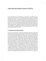
lines. The equivalent circuit of such a GUPFC, which is shown in Fig. 4.1, is used
to show the basic operation principle for the sake of simplicity. However, the
mathematical derivation is ap plicable to a GUPFC with an arbitrary number of se-

ries converters.
In the steady state o peration, the main o bjective of the GUPFC is to control
voltage and power flow. Real power can be exchanged among these shunt and se-
ries converters via the common DC link. The sum of the real power exchange
should be zero if we neglect the losses of the converter circuits.
114 4 Modeling of FACTS-Devices in Optimal Power Flow A nalysis
For the GUPFC shown in Fig. 4.1, it has total 5 degrees of control freedom, that
means it can control five power system quantities such as one bus voltage, and 4
active and reactive power flows of two lines. It can be seen that with more series
converters i ncluded within the GUPFC, more degrees of control freedom can be
introduced and hence more control objectives ca n be achieved.
In Fig. 4.1
i
Zsh and
in
Zse are the shunt and series transformer impedances,
respectively.
iii
șshVsh
∠=Vsh
and
ininin
șseVse
∠=Vse
( n=j,k) are the control-
lable injected shunt and series voltage sources.
i
PEsh and
in
PEse

are the power
exchange of the shunt converter and series converter, respectively, via the com-
mon DC link.
4.3.2.1 Power Flow Constraints of GU PFC
The power flow constraints of the GUPFC are summarized as follows:
Shunt power flows:
))sin()cos((
2
iiiiiiiiiii
shbshshgshVshVgshVPsh
θθθθ
−+−−=
(4.57)
))cos()sin((
2
iiiiiiiiiii
shbshshgshVshVbshVQsh
θθθθ
−−−−−=
(4.58)
Series power flows:
)sincos(
2
ininininniiniin
bgVVgVP
θθ
+−=
))sin()cos((
iniininiinini
sebsegVseV

θ
θ
θ
θ
−+−−
(4.59)
)cossin(
2
ininininniiniin
bgVVbVQ
θθ
−−−=
))cos()sin((
iniininiinini
sebsegVseV
θ
θ
θ
θ
−−−−
(4.60)
Fig. 4.1. The equivalent circuit of the GUPFC
4.3 Modeling of FACTS in O PF Analysis 115
))sin()cos((
2
ininininniinnni
bgVVgVP
θθθθ
−+−−=
))sin()cos((

innininnininn
sebsegVseV
θ
θ
θ
θ
−+−+
(4.61)
))cos()sin((
2
ininininninnnni
bgVVbVQ
θθθθ
−−−−−=
))cos()sin((
innininnininn
sebsegVseV
θ
θ
θ
θ
−−−+
(4.62)
where
)/1Re(
inin
g Zs e= , )/1Im (
inin
b Zse= .
in

P
,
in
Q
(n=j, k) a re the active and
reactive power flows of two GUPFC series branches leaving bus i while
ni
P
,
ni
Q
( n=j,k) are the active and reactive power flows of the GUPFC series branch
n-i leaving bus n (n=j,k), r espectively. Since two transmission lines are series
connected with the FACTS branches i-j, i-k via the GUPFC buses j and k, respec-
tively,
ni
P
,
ni
Q
(n=j,k) are equal to the active and reactive power flows at the
sending-end of the transmission lines, respectively.
The operating constraint representing the active power exchange among con-
vertersviathecommonDClinkis:
0
=−
¦
−=
dcini
PPEsePEshPEx

(4.63)
where n=j,k.
dc
P is the power loss of the DC circ uit of the GUPFC.
i
PEsh
and
in
PEse
satisfy the following equalities:
0)(Re- =
*
iii
PEsh IshVsh
(4.64)
0)(Re- =
*
niinin
PEse IVse
(4.65)
4.3.2.2 Operating Control Equalities of GUPFC
The GUPFC shown in Fig. 4.1 can control both active and reactive power flows of
the two transmission lines. The active and reactive power flow control constraints
of the GUPFC are given by (3.50) and (3.51)
The GUPFC has additional capability to c ontrol the voltage magnitude of bus i:
εε
+≤≤−⇔=−
Spec
ii
Spec

i
Spec
ii
VVVVV 0
(4.66)
where
i
V
is the voltage magnitude at bus i.
Spec
i
V
is the specified bus voltage con-
trol reference at bus i. In the point of view of the implementation, the inequality is
preferred since incorporation of the simple variable inequality is very easy.
4.3.2.3 Operating Inequalities of GUPFC
For t he operation of the GUPFC, the injected voltage sources should be within
their operating ratings while the currents through t he converters should be within
the current ratings:
116 4 Modeling of FACTS-Devices in Optimal Power Flow A nalysis
Shunt converter
maxmin
iii
shshsh
θθθ
≤≤
(4.67)
maxmin
iii
VshVshVsh ≤≤

(4.68)
maxmax
iii
PEshPEshPEsh ≤≤−
(4.69)
max
ii
IshIsh ≤
(4.70)
Series converter
maxmin
ininin
sesese
θθθ
≤≤
(4.71)
maxmin
ininin
VseVseVse ≤≤
(4.72)
maxmax
ininin
PEsePEsePEse ≤≤−
(4.73)
max
nini
II ≤
(4.74)
where n = j, k.
max

i
PEsh
is the maximum limit of the power exchange of the shunt
converter with the DC link.
max
i
Ish
is the current rating.
max
in
PEse
is the maximum
limit of the power exchange of the series converter with the DC link ( n=j,k).
max
ni
I
is the current rating of the series converter.
4.3.3 Incorporation of GUPFC into Nonlinear Interior Point OPF
4.3.3.1 Constraints of GUPFC
The GUPFC consists of the power flow constraints (4.57)-(4.62), the internal
power exchange balance constraint (4.63), the operating inequality constraints
(4.67)-(4.74), and the power flow c ontrol constraints and voltage control con-
straint (4.66). In the formulation of the nonlinear interior point OPF algorithm, the
power flow constraints (4.57)-(4.62) can be directly incorporated into the power
mismatch e quations at bus i, j and k. By introducing slack variables and barrier
parameter, the inequalities (4.67)-(4.74) can be converted into equalities. Then all
the transformed equalities of the GUPFC can be incorporated into the Lagrangian
function of the OPF problem.
4.3.3.2 Variables of GUPFC
The state variables of the GUPFC are

i
sh
θ
,
i
Vsh ,
i
PEsh ,
in
se
θ
,
in
Vse ,
in
PEse .
With incorporation of
i
PEsh
,
in
PEse
into the state variables of the GUPFC, the
formulation of the Newton OPF equation and the implementation of multi-control
4.3 Modeling of FACTS in O PF Analysis 117
functional model become simple and straightforward. In addition to the state vari-
ables, dual variables should be introduced for all the eq ualities and inequalities
while slack variables should be introduced for all the inequalities. In the imple-
mentation, the angle constraints (4.67) a nd (4.71) are optional since they are usu-
ally allowed to move around

$
360
. For the simplicity of presentation, the angle
constraints (4.67) and ( 4.71) are not discussed here.
The dual variables of the GUP FC inequality constraints are defined as follows:
:
i
lVsh
π
0
min
=−−
iii
SlVshVshVsh (4.75)
:
i
uVsh
π
0
max
=+−
iii
SuVshVshVsh (4.76)
:
i
lPEsh
π
0
min
=−−

iii
SlPEshPEshPEsh (4.77)
:
i
uPEsh
π
0
max
=+−
iii
SuPEshPEshPEsh (4.78)
:
i
uIsh
π
0
max
=+−
iii
SuIshIshIsh (4.79)
:
in
lVse
π
0
min
=−−
ininin
SlVseVseVse (4.80)
:

in
uVse
π
0
max
=+−
ininin
SuVseVseVse (4.81)
:
in
lPEse
π
0
min
=−−
ininin
SlPEsePEsePEse (4.82)
:
in
uPEse
π
0
max
=+−
iii
SuPEsePEsePEse (4.83)
:
ni
uIse
π

0
max
=+−
ninini
SuIseIseIse (4.84)
In the above equations, all the variables that start with ‘S’ are slack variables
and they are positive values while all the variables that start with ‘
π
’aredual
variables.
The dual variables of the eq ualities of the GUPFC are defined as foll ows:
:PEx
λ
0=
¦
+=
ini
PEsePEshPEx (4.85)
:
i
PEsh
λ
0)Re( =−
*
iii
PEsh IshVsh
(4.86)
:
in
PEse

λ
0)Re( =−
*
inniin
PEse IVse
(4.87)
:
ni
P
λ
0=−=∆
Spec
ni
nini
PPP
(4.88)
:
ni
Q
λ
0=−=∆
Spec
ni
nini
QQQ
(4.89)
:
m
p
λ

0=∆
m
P
(m = i, j,k)(4.90)
118 4 Modeling of FACTS-Devices in Optimal Power Flow A nalysis
:
m
q
λ
0=∆
m
Q (m = i, j,k) (4.91)
where
m
P∆
and
m
Q∆
are power mismatch equations at bus m.
4.3.3.3 Augmented Lagrangian Function of GUPFC in Nonlinear
Interior OPF
The augmented Lagrangian function of the equalities (4.75) -(4.84) is as follows:
)ln(equality* Sȝ−
π
(4.92)
The augmented Lagrangian function of the equalities (4.85)-(4.91) is defined as
follows:
mmmm
Spec
ni

nini
Spec
ni
nini
*
inininin
*
iiii
kjn
ini
QqPp
QQQPPP
PEsePEse
PEshPEshPEsePEshPEx
∆−∆−
−−−−
−−
−−
¦
−−
=
λλ
λλ
λ
λλ
)()(
))Re((
))Re(()(
,
IseVse

IshVsh
(n = j, k; m = i, j, k)
(4.93)
4.3.3.4 Newton Equation of Nonlinear Interior OPF with GUPFC
With the incorporation of the augmented Lagrangian functions above into the OPF
problem in section 4.2, a reduced Newton equation can be derived:
»
¼
º
«
¬
ª
=
»
»
¼
º
«
«
¬
ª
∆
∆
»
»
¼
º
«
«
¬

ª
b
a
x
x
BC
CA
sys
T
gupfc
(4.94)
where
T
]X,X,X[X
gupfc
i
gupfc
ij
gufc
ik
gupfc
∆∆∆=∆ - the incremental vec t or of the GUPFC
variables, and
T
],,,,,[X
niniininininni
gupfc
in
QsePsePEsePEseVseșseuIse
λλλπ

∆∆∆∆∆∆=∆ ,
-the
incremental vector of the variables of the GUPFC series branch in.
T
],,,,[X PExPEshPEshVshșshuIsh
iiiii
gupfc
i
λλπ
∆∆∆∆∆∆=∆ ,
- the incremental
vector of the variables of the GUPFC shunt branch i.
T
]X,X,X[X
sys
k
sys
j
sys
i
sys
∆∆∆=∆ - the incremental vector of the variables of the sys-
tem buses.
T
]a,a,a[a
iikij
= - the right hand vector of the GUPFC.
T
],,,[X
mmmm

sys
m
qpV
λλθ
∆∆∆∆=∆
(m = i, j, k) - the incremental vector of the
variables of system bus m.
4.3 Modeling of FACTS in O PF Analysis 119
In (4.94), all the slack and dual variables of the simple variable inequalities
have been eliminated from the formulation.
B and
b
are the system matrix and
right hand vector, which have similar structure to the system matrix and right hand
of (4.54), respectively except that in calculating the former, the contributions from
the GUPFC should be considered.
in
a
and
i
a
are given by
»
»
»
»
»
»
»
»

»
»
¼
º
«
«
«
«
«
«
«
«
«
«
¬
ª
∇−
∇−
∇−
−+∇−
−+∇−
∇−
∇−∇−
=
−
µλ
µλ
µλ
µ
µ

µθ
µµπ
µ
µ
π
L
L
L
SuPEseSlPEseL
SuVseSlVseL
L
LuIseL
in
in
in
in
in
in
inin
Qse
Pse
PEse
ininPEse
ininVse
se
SuIseinuIse
in
)/1/1(
)/1/1(
)(

1
a (n=j,k)
(4.95)
»
»
»
»
»
»
»
»
¼
º
«
«
«
«
«
«
«
«
¬
ª
∇−
∇−
−++∇−
−+∇−
∇−
∇−∇−
=

−
µλ
µλ
µ
µ
µθ
µµπ
µ
µ
π
L
L
SuPEshSlPEshL
SuVshSlVshL
L
LuIshL
PEx
PEsh
iiPEsh
iiVsh
sh
SuIshiuIsh
i
i
i
i
i
ii
)/1/1(
)/1/1(

)(
1
a
(4.96)
In (4.54), A and
C
are given by:
D
XX
A +
»
»
¼
º
«
«
¬
ª
∂∂
∂
=
gupfcgupfc
L
2
(4.97)
»
»
¼
º
«

«
¬
ª
∂∂
∂
=
sysgupfc
L
XX
C
2
(4.98)
where
D is given by:
[
]
iikij
Diag d,d,dD =
(4.99)
»
¼
º
«
¬
ª
−
−
=
0,0,0),//(
)//(,0,0

inininin
inininin
in
SuPEseuPEseSlPEselPEse
SuVseuVseSlVselVse
Diag
ππ
ππ
d
(n=j,k)
(4.100)
120 4 Modeling of FACTS-Devices in Optimal Power Flow A nalysis
»
¼
º
«
¬
ª
−
−
=
0,0),//(
)//(,0,0
iiii
iiii
i
SuPEseuPEseSlPEselPEse
SuVseuVseSlVselVse
Diag
ππ

ππ
d
(4.101)
Some of the first and seco nd terms of the Newton equation of the nonlinear in-
terior point OPF are given in the Appendix of this chapter.
4.3.3.5 Implementation of Multi-Configurations and Multi-Control
Functions of GUPFC
Multi-configurations of GUPFC. The GUPFC may have the configurations or
topologies such as GUPFC or SSSCs plus STATCOM.
For the GUPFC configuration, the operation of GUPFC is mainly constrained
by its voltage and current ratings of the converters and the active power exchange
of the converters with the D C link. For the SSSCs plus STATCOM configuration
the series converters are operated as SSSCs while the shunt converter is operated
as a STATCOM, there is active power exchange between the SSSCs and
STATCOM. The control configuration is simulated by setting the power exchange
limits to zero.
Multi-control functions of GUPFC. As discussed in chapter 3, there are a num-
ber of control objectives that can be achieved b y the series and shunt control. For
instance, in the implementation of other series control functions other than the ac-
tive and reactive power flow control, the latter can be simply replaced by the new
control equations. For the case of power flow control, the following control modes
may be adopted:
1. Active and reactive power flow control.
2. Active power flow control only.
3. Reactive power flow control only.
4. Without e xplicit active and reactive power control objectives.
For the implementation of 1, the dual variable of the reactive power flow control
constraint sh ould be dummied in the Newton equation of (4.94). Similarly by
dummying the releva nt dual variable in the Newton equation, the corresponding
control equation can be removed from the equation.

Noting the fact that an OPF is to optimize the system globally, the control mode
4. is more practical and useful. However, for power flow analysis, the active and
reactive power flow control equations must be retained.
4.3.3.6 Initialization of GUPFC Variables in Nonlinear Interior OPF
If the GUPFC has explicit series control objectives, then the initialization of the
series converters can be done in the same way as discussed in chapter 3 for the
GUPFC in power flow calculations. However, if there are no explicit objectives
applied, t hen the injected series voltage magnitude may be set to a value, say
1.0 upVse
in
= (n=j, k) while
i
Vsh is given by:
4.3 Modeling of FACTS in O PF Analysis 121
2/)(
minmax
iii
VshVshVsh += or
Spec
i
i
VVsh = (4.102)
4.3.4 Modeling of IPFC in Nonlinear Interior Point O PF
In comparison to the GUPFC, the IPFC has no shunt converter and the associated
control. For the IPFC s hown in Fig. 3.4 and Fig. 3.5, the primary series converter
i-j has two control degrees of freedom while the secondary series converter i-k has
one control degree of freedom since another control degree of freedom of the con-
verter is used to balance the active power exchange between the two series con-
verters. Very similar to that for the GUPFC, A reduced Newton equation for the
IPFC can be derived as follows:

»
¼
º
«
¬
ª
=
»
»
¼
º
«
«
¬
ª
∆
∆
»
»
¼
º
«
«
¬
ª
b
a
x
x
BC

CA
sys
T
gupfc
(4.103)
where
T
]X,X[X
ipfc
ik
ipfc
ij
ipfc
∆∆=∆
- the incremental vector of the I PFC variables, and
T
],,,,,,[X
jijiijijijijji
ipfc
ij
QsePsePEsePEseVseșseuIse
λλλπ
∆∆∆∆∆∆∆=∆ -the
incremental vector of the variables of the IPFC primary series branch ij.
T
],,,,,[X PExPsePEsePEseVseșseuIse
kiikikikikik
ipfc
ik
λλλπ

∆∆∆∆∆∆∆=∆ ,-the
incremental vector of the variables of the IPFC secondary series branch ik.
T
]X,X,X[X
sys
k
sys
j
sys
i
sys
∆∆∆=∆
- the incremental vector of the variables of the sys-
tem buses.
T
]a,a[a
ikij
= - the right hand vector of the IPFC
T
],,,[X
mmmm
sys
m
qpV
λλθ
∆∆∆∆=∆ (m = i, j, k) - the incremental vector of the
variables of system bus m.
In (4.103), all the slack and dual variables of the simple variable inequalities
have been eliminated from the formulation.
B and

b
are the system matrix and
right hand vector, which have similar structure to the system matrix and right hand
of (4.54), respectively except that in calculating the former, the contributions from
the IPFC should be considered.
ij
a
and
ik
a are given by:
122 4 Modeling of FACTS-Devices in Optimal Power Flow A nalysis
»
»
»
»
»
»
»
»
»
»
»
¼
º
«
«
«
«
«
«

«
«
«
«
«
¬
ª
∇−
∇−
∇−
−+∇−
−+∇−
∇−
∇−∇−
=
−
µλ
µλ
µλ
µ
µ
µθ
µµπ
µ
µ
π
L
L
L
SuPEseSlPEseL

SuVseSlVseL
L
LuIseL
ji
ji
ij
ij
ij
ij
ijij
Qse
Pse
PEse
ijijPEse
ijijVse
se
SuIseijuIse
ij
)/1/1(
)/1/1(
)(
1
a
(4.104)
»
»
»
»
»
»

»
»
»
»
»
»
»
»
»
»
»
¼
º
«
«
«
«
«
«
«
«
«
«
«
«
«
«
«
«
«

¬
ª
∇−
∇−
∇−
−+∇−
−+∇−
∇−
∇−∇−
=
−
µλ
µλ
µλ
µ
µ
µθ
µµπ
µ
µ
π
L
L
L
SuPEseSlPEseL
SuVseSlVseL
L
LuIseL
PEx
Pse

PEse
ikikPEse
ikikVse
se
SuIseikuIse
ik
ki
ik
ik
ik
ik
ikik
)/1/1(
)/1/1(
)(
1
a
(4.105)
SimilartothatoftheGUPFC,
A and C are given by:
D
XX
A +
»
»
¼
º
«
«
¬

ª
∂∂
∂
=
ipfcipfc
L
2
(4.106)
»
»
¼
º
«
«
¬
ª
∂∂
∂
=
sysipfc
L
XX
C
2
(4.107)
where
D is given by
[
]
ikij

Diag d,dD =
(4.108)
»
¼
º
«
¬
ª
−
−
=
0,0,0),//(
)//(,0,0
ijijijij
ijijijij
ij
SuPEseuPEseSlPEselPEse
SuVseuVseSlVselVse
Diag
ππ
ππ
d
(4.109)
»
¼
º
«
¬
ª
−

−
=
0,0,0),//(
)//(,0,0
ikikikik
ikikikik
ik
SuPEseuPEseSlPEselPEse
SuVseuVseSlVselVse
Diag
ππ
ππ
d
(4.110)
4.4 Modeling of Multi-Terminal VSC-HVDC in OPF 123
4.4 Mod eling of Multi-Terminal VSC-HVDC in OPF
4.4.1 Multi-Terminal VSC-HVDC in Optimal Voltage and Power Flow
The multi-terminal VSC-HVDC models for power flow analysis have been pre-
sented in chapter 3. A multi-terminal VSC-HVDC model suitable for optimal
power flow analysis will be discussed here. The multi-terminal VSC-HVDC has
not only power flow but also voltage control capability. It is useful to compare the
GUPFC with the M-VSC-HVDC and investigate different control capabilities of
these two FACTS-devices.
The equivalent circuit of the multi-terminal VSC-HVDC (M-VSC-HVDC) is
shown in Fig. 4.2. In this figure, for the sake of simplicity, the VSC HVDC con-
sists of three terminals. However, the derivation is applicable to a M-VSC-HVDC
with any number of terminals.
As discussed in chapter 3, the M-VSC-HVDC combining three or more con-
verters working together extends the concepts of voltage and power flow control
beyond what is achievable with the known two-converter VSC-HVDC-device.

The simplest M-VSC-HVDC consists of three converters connected in sh unt with
two buses in a substation. It can control total five power system quantities such as
a bus voltage of the secondary converter and independent active and reactive
power flows of two lines, which are connected with the primary converters.
In the s teady state operation, the main objective of the M-VSC-HVDC is to
control voltage and power flow. Real pow er can be exchanged among these con-
verters via the common DC link. The s um of t he real power exchange should be
zero if we neglect the losses of the converter circuits. For the M-VSC-HVDC
shown in Fig. 4.2, if explicit controls are applied, it has tot al 5 degrees of control
freedom, that means it can control five power system quantities such as one bus
voltage, and 4 active and reactive power flows of two lines. It can be seen that
with more converters included within the M-VSC-HVDC, more degrees of control
freedom can be intro duced and hence more co ntrol objectives can be achieved.
4.4.2 Operating and Control Constraints of the M-VSC-HVDC
In Fig. 4.2, the AC power flow constraints of the M-VSC-HVDC at buses i, j, k
can be explicitly incorporated into the power mismatch equations at these AC
buses.
The active power exchange among the converters via the DC link should be
balanced at any instant, which is described by:
0=+++= PlossPdcPdcPdcPEx
kji
(4.111)
where
Plos
s
represents losses in converter circuits. The handling of Ploss has
been discussed in chapter 3.
124 4 Modeling of FACTS-Devices in Optimal Power Flow A nalysis
m
Pdc (m=i,j,k) as shown in Fig. 4.2 is the power exchange of the converter with

the DC link and can be described by the f ollowing equalities:
0)Re(- =−
*
mmm
Pdc IshVsh m = i, j, k
(4.112)
where
))sin()cos(()Re(
2
mimmimmimm
*
mm
shbshshgshVshVgshVsh
θθθθ
−−−−=− IshVsh .
Voltage and power flow control constraints of the M-VSC-HVDC consists of
explicit PQ or P V control of primary converters as given by (3.79)-(3.82) and
voltage control of secondary converter. I n the implementation of the voltage con-
trol, the equality i s simply replaced by an inequality of bus voltage constraint
since the im plem entation of the simple variable inequality constraint is very sim-
ple and straightforward.
In addition to the a bove equality constraints, voltage and current inequality
constraints of the M-VSC-HVDC as shown in (3.84) and (3.85) should be consid-
ered.
4.4.3 Modeling of M-VSC-HVDC in the Nonlinear Interior Point OPF
Following the similar procedure in the deri vation of Nonlinear Interior Point OPF
with incorporation of the GUPFC, a reduced Newton equation can be obtained:
With the incorporation of the augmented Lagrangian functions above into the
OPF problem in section 4.2, a r educed Newton equation can be derived:
»

¼
º
«
¬
ª
=
»
»
¼
º
«
«
¬
ª
∆
∆
»
»
¼
º
«
«
¬
ª
b
a
x
x
BC
CA

sysT
HVDC
(4.113)
where
Fig. 4.2. The equivalent circuit of the multi-terminal VSC HVDC
4.4 Modeling of Multi-Terminal VSC-HVDC in OPF 125
T
]X,X,X[X
HVDC
k
HVDC
j
HVDC
i
HVDC
∆∆∆=∆
- the incremental vector of the M-
VSC-HVDC variables, and
T
],,,,[X PExPEshPEshVshșshuIsh
iiiii
HVDC
i
λλπ
∆∆∆∆∆∆=∆ , - the incremental
vector of the variables of the M-VSC-HVDC branch i.
T
],,,,[X
jjjjjjj
HVDC

j
QEshPEshPEshPEshVshșshuIsh
λλλπ
,, ∆∆∆∆∆∆=∆ -the
incremental vector of the variables of the M-VSC-HVDC branch j.
T
],,,,[X
kkkkkkk
HVDC
k
QEshPEshPEshPEshVshșshuIsh
λλλπ
,, ∆∆∆∆∆∆=∆
the
incremental vector of the variables of the M-VSC-HVDC branch k.
T
]X,X,X[X
sys
k
sys
j
sys
i
sys
∆∆∆=∆ - the incremental vector of the variables of the sys-
tem buses.
T
]a,a,a[a
kji
= -therighthandvectorof theM-VSC-HVDC.

T
],,,[X
mmmm
sys
m
qpV
λλθ
∆∆∆∆=∆
(m = i, j, k) - the incremental vector of the
variables of system bus m.
In (4.113), all the slack and dual variables of the simple variable inequalities
have been eliminated from the formulation.
B and
b
are the system matrix and
right hand vector have similar structure to the system matrix and right hand of
(4.54), respectively except that in calculating the former, the contributions from
the M-VSC-HVDC should be considered.
i
a
and
m
a
are given by:
»
»
»
»
»
»

»
»
¼
º
«
«
«
«
«
«
«
«
¬
ª
∇−
∇−
−++∇−
−+∇−
∇−
∇−∇−
=
−
µλ
µλ
µ
µ
µθ
µµπ
µ
µ

π
L
L
SuPEshSlPEshL
SuVshSlVshL
L
LuIshL
PEx
PEsh
iiPEsh
iiVsh
sh
SuIshiuIsh
i
i
i
i
i
ii
)/1/1(
)/1/1(
)(
1
a
(4.114)
»
»
»
»
»

»
»
»
»
»
¼
º
«
«
«
«
«
«
«
«
«
«
¬
ª
∇−
∇−
∇−
−+∇−
−+∇−
∇−
∇−∇−
=
−
µλ
µλ

µλ
µ
µ
µθ
µµπ
µ
µ
π
L
L
L
SuPEshSlPEshL
SuVshSlVshL
L
LuIshL
m
m
m
m
m
m
mm
Qsh
Psh
PEsh
mmPEsh
mmVsh
se
SuIshmuIsh
m

)/1/1(
)/1/1(
)(
1
a (m=j,k)
(4.115)