minitab drawing statistics chart
Bạn đang xem bản rút gọn của tài liệu. Xem và tải ngay bản đầy đủ của tài liệu tại đây (2.35 MB, 42 trang )
DRAWING STATISTICS CHART– MINITAB
Lesson 1 At the AB battery factory, KCS staff measured the weight (g) of 10 plates
during the first casting and recorded the following data:
9.46; 10.61; 8.07; 12.21; 9.02 ; 8.99; 10.03; 11.73; 10.99; 10.56
Determine the values: mean, standard deviation, variance, median.
Draw a chart with the above data
Solution:
- Import data in Minitab:
-Go to Stat / Basic statistic / Display Discripitive Statistic
1
- Click the box Variables: Select C1 and press Select
- Click the Statistics button: select the Mean parameters; Standard deviation; Variance;
Median
-Click OK
2
-Chọn màn hình Session xem kết quả:
Draw a Run chart:
-Go to Stat/ Quality tool/ Run chart
3
- In the Data Arranged as:
Item Single Column: press C1 and press Select
Item Subgroup Size: press C1 and click OK
-Resulut:
4
Similar exercises:
Draw a Run chart for the price recording data of a scarce commodity as follows:
Date
1
2
3
4
5
6
7
8
9
10
11
12
13
14
15
16
17
18
19
20
Price
35
38
41
43
47
43
48
52
53
55
59
56
52
55
59
63
61
62
65
67
Bài 2: Draw a graph of the thickness distribution (mm) of the sheets as follows:
8.02; 8.15; 7.89; 7.95; 7.77; 8.20; 7.79; 7.90; 8.02; 8.06; 7.86; 7.92; 8.04; 7.98; 8.01; 8.06;
7.80; 7.96; 7.95; 8.15; 8.02
Solution:
-
Data input
5
-Go to Graph \ Histogram
-
Lelect With Fit and press OK
6
-At the item Graph Variables: select C1 and press OK
Similar exercises:
7
Plot the Hitogram chart for recording data set “Thickness (mm) of corrugated iron as follows”
3.56
3.48
3.41
3.55
3.48
3.59
3.4
3.48
3.52
3.41
3.46
3.56
3.37
3.52
3.48
3.63
3.54
3.5
3.48
3.45
3.48
3.5
3.47
3.44
3.32
3.59
3.46
3.56
3.46
3.34
3.5
3.52
3.49
3.5
3.40
3.47
3.51
3.50
3.45
3.44
3.42
3.47
3.45
3.45
3.52
3.38
3.48
3.52
3.46
3.47
3.43
3.48
3.44
3.44
3.54
3.52
3.50
3.46
3.54
3.47
3.52
3.46
3.50
3.48
3.46
3.45
3.68
3.48
3.54
3.41
3.49
3.50
3.49
3.46
3.43
3.48
3.60
3.46
3.48
3.48
3.44
3.56
3.46
3.52
3.30
3.31
3.46
3.52
3.49
3.54
3.5
3.38
3.46
3.46
3.46
3.46
3.52
3.56
3.41
3.47
Bài 3: Draw a Scatter chart for the data collected in the laboratory as follows:
PhH2O
Độ
axit
6.92
6.59
7.14
7.1
6.91
7.3
6.64
6.74
6.58
6.1
5.84
5.21
6.98
7.08
6.98
5.3
7.3
7.41
6.12
2.95
2.70
2.65
2.7
2.7
2.55
2.5
2.8
2.4
2.5
2.35
2.7
2.4
2/5
2.55
2.55
2.3
2.4
2.3
Solution:
-Import data:
-Go to Graph \ Scatterplot
8
-Choose With Regression, press OK
-At box Y-Variables select “ Ph-nước”; X-Variables select “ Độ axit”; press Ok
9
Result:
- Find the regression equation and the correlation coefficient R:
10
Go to Stat \ Regression \ Regression
-In the box Response : select “ Ph nước”; box Predictor select “ Độ axit”, click Result
select “ Regression equation , table of coefficients…”
11
- In the session window, see the results :
Similar exercises
12
Scatterplot drawing; Find the regression equation and the correlation coefficient R for the data
collected about an automobile engine as follows:
Speed
(km/h)
Gas (l)
30
30
35
35
40
40
45
45
50
50
55
55
60
60
65
65
38
35
35
30
33
28
32
29
26
26
32
21
22
22
18
24
Lesson 4: Control Chart X bar- R
At one stage in the steel plant, KCS staff took samples to check the diameter of steel
pipes (mm) at different times and recorded the data as follows:
Results
Samples
1
6h
14
10h
12.6
14h
13.2
18h
13.1
22h
12.1
2
13.2
13.3
12.7
13.4
12.1
3
13.5
12.8
13
12.8
12.4
4
13.9
12.4
13.3
13.1
13.2
5
13
13
12.1
12.2
13.3
6
13.7
12
12.5
12.4
12.4
7
13.9
12.1
12.7
13.4
13
8
13.4
13.6
13
12.4
13.5
9
14.4
12.4
12.2
12.4
12.5
10
13.3
12.4
12.6
12.9
12.8
11
13.3
12.8
13
13
13.1
12
13.6
12.5
13.3
13.5
12.8
13
13.4
13.3
12
13
13.1
14
13.9
13.1
13.5
12.6
12.8
15
14.2
12.7
12.9
12.9
12.5
16
13.6
12.6
12.4
12.5
12.2
17
14
13.2
12.4
13
13
18
13.1
12.9
13.5
12.3
12.8
13
Results
Samples
19
6h
14.6
10h
13.7
14h
13.4
18h
12.2
22h
12.5
20
13.9
13
13
13.2
12.6
21
13.3
12.7
12.6
12.8
12.7
22
13.9
12.4
12.7
12.4
12.8
23
13.2
12.3
12.6
13.1
12.7
24
13.2
12.8
12.8
12.3
12.6
25
13.3
12.8
12
12.3
12.2
Draw process control charts; calculate Cp, Cpk knowned USL = 13.8; LSL = 12.1
Solution:
- Enter data in Minitab
-Go to Stat/ Control Chart/ Variables chart for subgroubs/ X bar-R
14
-Select Observation for a subgroups are in one row of columns
-Select from C1 đến C5 and press Select
- Select X-bar R options ;
15
-Go to Estimate : in the box of Method for estimating standard deviation select Rbar; click
OK
-Result of Control chart Xbar-R
-Calculate Cp; Cpk
16
Go to Stat\Quality tool\ Capability Analysis\ Normal
-Select Subgroubs across row of: select from C1 to C5, press Select
-Input data Lower spec = 12.1; Upper Spec= 13.8
-Results:
17
-
Result of Overall Capability : Cp= 0.52; Cpk= 0.51
Similar exercises
At the wire factory, KCS staff checks the weight (g) of the wire samples and records the
following data:
STT
Sample
1
2
3
4
5
6
7
8
9
10
11
12
13
14
15
X1
15
17
12
42
32
26
32
23
15
32
31
25
32
18
24
X2
24
37
22
35
26
17
19
27
24
31
29
23
32
22
25
X3
24
28
30
29
24
28
21
31
28
24
27
26
31
19
26
X4
20
26
36
36
19
25
25
31
27
25
24
28
29
23
22
X5
25
26
34
22
31
22
27
24
31
22
26
30
28
26
28
a) Calculate the average and control limits of the Xbar-R chart
b. Draw control charts; compute Cp and Cpk know USL = 28.1 and LSL = 11.9
Bài 5: Biểu đồ kiểm soát Xbar-S
18
KCS staff checked the weight (g) of the Hura cake samples, each time this staff took 7
samples and recorded the data in 15 groups which were taken as follows:
Stt
Sample
X1
X2
X3
X4
X5
X6
X7
1
110
83
99
98
109
99
98
2
3
4
5
6
7
8
9
10
11
12
13
14
15
103
97
96
105
110
100
93
103
97
103
90
97
99
106
95
110
102
110
91
96
90
105
93
97
100
101
106
94
109
90
105
109
104
104
110
109
93
104
91
96
97
96
95
97
90
93
91
93
108
90
99
103
103
104
105
98
96
100
96
98
101
96
105
108
96
92
105
108
98
90
101
102
88
97
105
106
98
103
105
100
108
95
92
100
95
97
90
93
98
101
96
105
97
103
90
104
110
90
a) Calculate the average and control limits of the Xbar-S chart
b) Draw Xbar-S Control Chart
-Import Minitab data
-Go to Stat/ Control charts/ Variables charts for Subgroups/
Xbar-S
19
- Select Observation for a subgroups are in one rows of columns; select X1 to X7, press Select
-Select Xbar S options
-Go to Estimate , chọn Method for estimating standard deviation, click
Sbar
20
-Press Ok : Chart result
Similar exercises
21
At the XYZ toothbrush factory, KCS staff checked the weight of the brush through 1
production stage, this staff took 6 samples in 1 inspection and conducted 15 checks. The data
was recorded as follows:
Stt
Sample
1
2
3
4
5
6
7
8
9
10
11
12
13
14
15
X1
15
17
12
42
32
26
32
23
15
32
31
25
32
18
24
X2
24
37
22
35
26
17
19
27
24
31
29
23
32
22
25
X3
24
28
30
29
24
28
21
31
28
24
27
26
31
19
26
X4
20
26
36
36
19
25
25
31
27
25
24
28
29
23
22
X5
25
26
34
22
31
22
27
24
31
22
26
30
28
26
28
X6
37
22
35
29
24
28
31
27
25
24
24
37
22
19
25
a) Calculate the average limit and control limits of the Xbar-S chart
b) Draw control chart Xbar-S
Lesson 6: I-MR Chart
Record of free acetic acid content during the reaction process:
Date
Sample
Result
01.10
1
1.09
02.10
2
1.13
03.10
3
1.29
04.10
4
1.13
05.10
5
1.23
06.10
6
1.43
07.10
7
1.27
08.10
8
1.63
09.10
9
1.34
10.10
10
1.1
11.10
11
0.98
12.10
12
1.37
22
Date
Sample
Result
13.10
13
1.18
14.10
14
1.58
15.10
15
1.31
16.10
16
1.7
17.10
17
1.45
18.10
18
1.19
19.10
19
1.33
20.10
20
1.18
21.10
21
1.40
22.10
22
1.68
23.10
23
1.58
24.10
24
0.9
25.10
25
1.7
26.10
26
0.95
a) Calculate the average limit and control limits of the I-MR chart
b. Drawing I-MR Control Chart Problem
Solving
-Import minitab data
-Go to Stat\ Control chart\Variables chart for Individual\I-MR
23
-In the box of Variables, select C1 press Select
-Click I-MR options: go to Estimate select Method for estimating standard deviation; click
select Average moving range and Length of moving = 2; press OK
24
Kết quả:
25