Short selling stocks with ConnorsRSI (2013)
Bạn đang xem bản rút gọn của tài liệu. Xem và tải ngay bản đầy đủ của tài liệu tại đây (759.86 KB, 39 trang )
Connors Research Trading Strategy Series
Short Selling Stocks
with ConnorsRSI
By
Connors Research, LLC
Laurence Connors
Cesar Alvarez
Matt Radtke
P a g e | 2
Copyright © 2013, Connors Research, LLC.
ALL RIGHTS RESERVED. No part of this publication may be reproduced, stored in a
retrieval system, or transmitted, in any form or by any means, electronic, mechanical,
photocopying, recording, or otherwise, without the prior written permission of the
publisher and the author.
This publication is designed to provide accurate and authoritative information in regard
to the subject matter covered. It is sold with the understanding that the author and the
publisher are not engaged in rendering legal, accounting, or other professional service.
Authorization to photocopy items for internal or personal use, or in the internal or
personal use of specific clients, is granted by Connors Research, LLC, provided that the
U.S. $7.00 per page fee is paid directly to Connors Research, LLC, 1-973-494-7333.
ISBN 978-0-9886931-5-9
Printed in the United States of America.
This document cannot be reproduced without the expressed written permission of Connors Research, LLC.
P a g e | 3
Disclaimer
By distributing this publication, Connors Research, LLC, Laurence A. Connors, Cesar Alvarez, and Matt
Radtke (collectively referred to as “Company") are neither providing investment advisory services nor
acting as registered investment advisors or broker-dealers; they also do not purport to tell or suggest
which securities or currencies customers should buy or sell for themselves. The analysts and employees
or affiliates of Company may hold positions in the stocks, currencies or industries discussed here. You
understand and acknowledge that there is a very high degree of risk involved in trading securities and/or
currencies. The Company, the authors, the publisher, and all affiliates of Company assume no
responsibility or liability for your trading and investment results. Factual statements on the Company's
website, or in its publications, are made as of the date stated and are subject to change without notice.
It should not be assumed that the methods, techniques, or indicators presented in these products will be
profitable or that they will not result in losses. Past results of any individual trader or trading system
published by Company are not indicative of future returns by that trader or system, and are not indicative
of future returns which be realized by you. In addition, the indicators, strategies, columns, articles and all
other features of Company's products (collectively, the "Information") are provided for informational and
educational purposes only and should not be construed as investment advice. Examples presented on
Company's website are for educational purposes only. Such set-ups are not solicitations of any order to
buy or sell. Accordingly, you should not rely solely on the Information in making any investment. Rather,
you should use the Information only as a starting point for doing additional independent research in order
to allow you to form your own opinion regarding investments.
You should always check with your licensed financial advisor and tax advisor to determine the suitability
of any investment.
HYPOTHETICAL OR SIMULATED PERFORMANCE RESULTS HAVE CERTAIN INHERENT
LIMITATIONS. UNLIKE AN ACTUAL PERFORMANCE RECORD, SIMULATED RESULTS DO NOT
REPRESENT ACTUAL TRADING AND MAY NOT BE IMPACTED BY BROKERAGE AND OTHER
SLIPPAGE FEES. ALSO, SINCE THE TRADES HAVE NOT ACTUALLY BEEN EXECUTED, THE
RESULTS MAY HAVE UNDER- OR OVER-COMPENSATED FOR THE IMPACT, IF ANY, OF CERTAIN
MARKET FACTORS, SUCH AS LACK OF LIQUIDITY. SIMULATED TRADING PROGRAMS IN
GENERAL ARE ALSO SUBJECT TO THE FACT THAT THEYARE DESIGNEDWITH THE BENEFIT OF
HINDSIGHT. NO REPRESENTATION IS BEING MADE THAT ANY ACCOUNT WILL OR IS LIKELY TO
ACHIEVE PROFITS OR LOSSES SIMILAR TO THOSE SHOWN.
Connors Research
10 Exchange Place
Suite 1800
Jersey City, NJ 07302
This document cannot be reproduced without the expressed written permission of Connors Research, LLC.
P a g e | 4
Table of Contents
Section 1 Introduction ............................................................................. 5
Section 2 Shorting Mechanics .................................................................. 8
Section 3 Strategy Rules ......................................................................... 11
Section 4 Test Results ............................................................................ 18
Section 5 Selecting Strategy Parameters ............................................... 24
Section 6 Using Options ......................................................................... 28
Section 7 Additional Thoughts ............................................................... 31
Appendix: The ConnorsRSI Indicator ..................................................... 33
This document cannot be reproduced without the expressed written permission of Connors Research, LLC.
P a g e | 5
Section 1
Introduction
This document cannot be reproduced without the expressed written permission of Connors Research, LLC.
P a g e | 6
For more than thirty years, the asset management industry has attempted to create firms and funds
revolving around short selling stocks. Few (very few) have succeeded in the long term. Most of these
funds (many now defunct) applied a single‐minded approach to short selling: identify a company that is
going out of business and short it.
For example, a well‐known short strategy is to find the firms that are committing accounting fraud and
short them. In the mid‐90s I paid $10,000 for a one‐year subscription to a research firm that specialized
in identifying accounting fraud. The report that subscribers received spelled out in detail the depth of
the accounting fraud a firm was committing. It was compelling. So compelling that of course I shorted
many of these stocks. Unfortunately, the 1995 bull market began to take hold and in zero cases were
any of these companies found to have committed fraud. In fact, many of these stocks experienced high
double‐digit (and in some cases triple‐digit) gains over the next year. Fortunately, I was out of all of
them before they maxed out; I was either stopped out by my own sense of panic or simply because my
put options went to zero. Over the years, this research company identified about 200 suspect firms, of
which three actually committed fraud. I was not a happy subscriber, nor were the many short or
long/short funds who also subscribed. Needless to say, I didn’t renew.
There are other strategies which have been used by short funds looking for companies to go to zero:
technologies that would become obsolete, competitors that would crush them, or the fact that the US
economy was going to collapse and therefore every company along the way would collapse as well.
None of these methods have worked in the long term. Yes, some companies have been found to have
committed fraud (Enron, Tyco, etc.), yes the US economy got hit in 2000‐2002 and in 2008, but overall
the performance of the majority of these short funds has been pretty dismal. The people behind these
funds mean well. Most have conviction in their beliefs. But their track record proves just how difficult it
is to make money in the long run by shorting stocks.
In this Strategy Guidebook, we’re going to teach you a quantitative, systematic way to short stocks that
has proven to be successful for quite some time. There are no juicy stories here. This strategy is simply
identifying behavior, backed by statistics, which has occurred over and over again since 2001. In fact we
can show you this same behavior going all the way back to 1995. The basic behavior pattern is: when
stocks become extremely overbought on a short‐term basis they tend to pull back sharply for a short
period of time. Few go out of business. However, most do pause, profit taking occurs, scared (long
speculative) money gets flushed out, further pressure is placed on the stock as analysts’ price targets get
hit, and in the majority of cases (approximately 70%, which is high) prices are lower within a few days.
We first identified this behavior in 2003 and started teaching a variation of the strategy in our
TradingMarkets Swing Trading College in 2005 which we still teach today. The concepts we taught back
then still hold true today and we’re proud of the fact that in spite of markets changing, especially after
2008, the behavior of extremely overbought stocks has not changed. And this is where the Alpha is.
A few words of caution need to be made here. First, these are short sales, which means that the losses
are potentially unlimited. Stops lower the test results but that doesn’t mean they should not be used;
that’s up to you. The test results include all stocks which have met the entry criteria for the strategy, and
This document cannot be reproduced without the expressed written permission of Connors Research, LLC.
P a g e | 7
some have risen by 50% ‐ 100% before exiting. On an individual trade basis this hurts. But as you see on
an overall basis, in spite of these adverse moves, the longer term test results are significantly
positive. For those of you who understand the risks involved in options, liquid puts can also be used to
contain the potential for unlimited losses, because your risk (total dollar amount) is known ahead of
time.
In order to achieve Alpha, you have to go places others won’t go. Shorting the stocks in this strategy is a
place most people psychologically can’t go. The edges have been there, as you will see in the statistics,
but you have to be able to overcome the fear of shorting “story stocks” which have been run up to
unsustainable short‐term levels by “the crowd”. This Guidebook, backed by over a decade of statistics,
will show you how to do this.
We hope you enjoy this next installment of the Connors Research Strategy Guidebook Series. If you
would like to see more topics from our Strategy Research Series please click here.
This document cannot be reproduced without the expressed written permission of Connors Research, LLC.
P a g e | 8
Shorting Mechanics
Section 2
This document cannot be reproduced without the expressed written permission of Connors Research, LLC.
P a g e | 9
Many individual investors will never short a stock. Sometimes this is because of the fear of associated
with swimming against the current, as described earlier in the Introduction. In other cases, it’s simply a
lack of adequate knowledge about how the process works. In this section, we’ll present some of the
basics that you should be familiar with before executing your first short sale.
We’re all quite accustomed to the model where we purchase something first and sell it later. Certainly
this is the case for most of the major investments we make in life, including houses, cars, artwork,
precious metals, etc. However, in certain financial transactions, we’re allowed to reverse the process by
selling something before we buy it. In the case of stocks, we call this short selling, or sometimes simply
shorting.
Every stock transaction involves a buyer who is willing to give up cash (either her own, or loaned to her
by a broker) in exchange for stock held by the seller. So how does the short seller complete this
transaction without actually owning any stock? Just as a buyer can use account margin to effectively
borrow cash from a broker, so too can the short seller borrow shares from his broker. If your broker has
shares that they are willing to loan to you for shorting, your trading platform will typically designate
those stocks as Easy to Borrow, or simply ETB. Stocks that are listed as Hard to Borrow, or HTB, may be
completely unavailable, or may require a call to a live person at your broker’s trade desk.
When we exit a short trade, we say that we are covering our position. We do this by buying the stock
(i.e. we give up cash in exchange for shares), but the shares we get don’t stay in our account, they go
back to the broker to repay the loan that was created when we entered the short position.
It’s worth noting that different brokers may have different stocks available to borrow. Very highly liquid
stocks will probably be ETB from most any broker, but less liquid stocks may be available from some
brokers and not others. If your current broker consistently doesn’t allow you to borrow shares that you
want to short, consider opening an account with another broker.
Because your broker is loaning you shares when you enter a short sale, you must have a margin account
with the brokerage firm. You cannot short stocks from an IRA, 401k, or other cash‐secured account.
Also, just like when you trade on margin, the broker will charge you interest on the shares you’ve
borrowed.
If you buy a stock for $100 per share, your maximum risk is the $100 you paid because the stock price
cannot go lower than zero. However, if you short a stock, your risk is potentially unlimited, because
theoretically there is no upper bound on the price. Keep in mind that if you’re in a short position and the
price moves against you, your broker will require you to have sufficient collateral (cash and other
securities) in your account to cover your position. Again, this is very similar to how your broker handles
long positions that you purchased using margin.
Another issue to be aware of is that short sellers are responsible for paying dividends. Let’s say that I
borrow a stock from my broker, and sell it short at $50/share. A few days later, the company pays a
$1/share dividend to the new owner, which will cause the stock price to drop by $1. However, my
broker still owns shares as well, because they simply lent them to me for a period of time. Since they
This document cannot be reproduced without the expressed written permission of Connors Research, LLC.
P a g e | 10
expect to collect their $1/share dividend as well, the money to pay that dividend comes out of my
account. Of course, if I shorted the stock at $50/share and cover it a few days later at $49/share, then
I’ve made $1/share on the transaction, and that’s the $1/share that pays the dividend. In other words,
when a company pays a dividend and the stock price falls by the corresponding amount, there is really
no net effect on the short seller other than the cash coming out of his or her account now versus the
gain that won’t be realized until the short position is covered.
Now that we’ve covered some of the basics around shorting, let’s move on to the rules for the strategy.
This document cannot be reproduced without the expressed written permission of Connors Research, LLC.
P a g e | 11
Strategy Rules
Section 3
This document cannot be reproduced without the expressed written permission of Connors Research, LLC.
P a g e | 12
The fundamental concept behind the ConnorsRSI Short Stock Strategy is to find stocks that have moved
strongly upward and achieved new short‐term highs. We short these stocks on further intraday strength,
and then wait for mean reversion to pull the prices back down before we exit.
This strategy executes trades using a simple three‐step process consisting of Setup, Entry and Exit. The
rules for each of these steps are detailed below.
A Setup occurs when all of the following conditions are true:
1. The stock’s price closes above $5 per share.
2. The average volume over the past 21 trading days (approximately one month) is greater
than 500,000 shares.
3. The stock closes with a ConnorsRSI(3,2,100) value greater than X,
where X is 75, 80, 85, 90 or 95.
4. The stock’s 100‐day Historical Volatility, or HV(100), is greater than 40.
5. The stock’s 10‐day Average Directional Index, or ADX(10), value is greater than 40.
6. Today’s High is the highest high in the past N days, where N is 7, 10 or 13.
If the previous day was a Setup, then we Enter a trade by:
7. Submitting a limit order to short the stock at a price Y % above yesterday’s close,
where Y is 2, 4, 6, 8, or 10.
NOTE: Some variations use Variable Limits. This concept will be explained in detail below.
After we’ve entered the trade, we Exit using one of the following methods, selected in advance:
8a. The stock closes with a ConnorsRSI value less than 20.
8b. The stock closes with a ConnorsRSI value less than 30.
8c. The stock closes with a ConnorsRSI value less than 40.
8d. The closing price of the stock is less than the 5‐day moving average, or MA(5).
8e. The closing price of the stock is lower than the previous day’s close. We typically refer to
this exit as the First Down Close.
Let’s look at each rule in a little more depth, and explain why it’s included in the strategy.
Rules 1 & 2 assure that we’re trading liquid stocks which are likely to have shares available to borrow.
Rule 3 uses ConnorsRSI to identify a price surge. A complete description of ConnorsRSI can be found in
the Appendix.
Rule 4 helps select stocks that have been experiencing healthy levels of price volatility over the past
several months. Short term strategies like the one presented here depend on strong price moves both
to set up the trade and to generate profits. Stocks with lower volatility are less likely to generate such
moves.
This document cannot be reproduced without the expressed written permission of Connors Research, LLC.
P a g e | 13
Rule 5 uses the ADX indicator to identify stocks that have been trending strongly. Although ADX is non‐
directional, the other rules assure us that the price has been moving upward, and thus ADX measures
the strength of that upward trend.
Rule 6 identifies an N‐day high. Stocks seldom move in one direction for an extended period of time, and
when the price reaches a short‐term high, it’s often a sign that the stock is getting ready to pull back
before resuming its upward trend.
Rule 7 allows us to enter the trade at an optimal price. The Setup rules identify an overbought stock,
and the entry rule waits for it to become even more overbought on an intraday basis. Because the
intraday price surge is occurring for a second consecutive day, it often motivates traders with long
positions to take some profits by closing their positions. Their selling will generate downward pressure
on the price, which in turn will generate profits for our short position.
Over the years, our research has consistently shown that stocks that are trading above their 200‐day
moving average, or MA(200), have a greater tendency to move upward in price, while stocks below their
MA(200) have a greater tendency to move downward. Using Variable Limit Entries allows us to leverage
this information by specifying a larger limit order when the stock is above the MA(200).
Strategy variations that use Variable Limit Entries use a limit percentage that is 1.5 times the standard
limit when the stock is above the MA(200). For example, if we’re using a variation with a stated limit
percentage (Y) of 4%, then a stock that closed above the MA(200) on the Setup day will actually use a
6% limit order to enter the trade, while a stock trading below the MA(200) will use the 4% limit. Strategy
variations that do not utilize Variable Limit Entries use the same limit percentage regardless of whether
the price on the Setup day closes above or below the MA(200). We will see examples of both kinds of
trades later in this section.
Rule 8 provides a well‐defined exit method. Few strategies have quantified, structured, and disciplined
exit rules. Rule 8 gives you the exact parameters to exit the trade, backed by over twelve years of
historical test results. As with all other strategy parameters, we select in advance the type of exit that
we will use, and apply that rule consistently in our trading.
In our testing we closed all trades at the close of trading on the day that the Exit signal occurred. If this is
not an option for you, our research has generally shown that similar results are achieved if you exit your
positions the next morning.
Now let’s see how a typical trade looks on a chart. For the example below, we’ll use a strategy variation
that requires the ConnorsRSI value to be above 90 and that requires a 10‐day high on the Setup day. The
limit order will be placed 6% above the Setup day’s closing price (no variable limits). We will exit when
ConnorsRSI closes below 30. In terms of our strategy rules above, that means X = 90, N = 10, Y = 6, and
the exit method is defined by Rule 8b.
This document cannot be reproduced without the expressed written permission of Connors Research, LLC.
P a g e | 14
Chart created in Amibroker. Reprinted courtesy of AmiBroker.com.
Figure 1: Zillow Trade
The chart above is for Zillow Inc., whose symbol is Z. In the chart, the top pane shows the price bars in
black and the 200‐day moving average or MA(200) in dark green. The vertical blue‐gray line marks the
currently selected day which is also the Setup day, February 14, 2013. The red down arrow marks the
entry day, and the green up arrow indicates the exit day. The middle pane shows the values for
ConnorsRSI in bright blue, 100‐day historical volatility or HV(100) in purple and ADX(10) in bright green.
The bottom pane shows the daily volume as a blue‐gray histogram, and the 21‐day average volume as a
turquoise line. Now we’ll confirm that each of our entry and exit conditions was correctly met.
Rule 1 requires the stock price to close above $5 on the Setup day. The closing price of $42.30 meets
this requirement.
Rule 2 is satisfied because the 21‐day average volume is over 725,000 shares, which is well above our
minimum requirement of 500,000 shares.
Based on our strategy parameters, Rule 3 requires the ConnorsRSI(3,2,100) value to be above 90 on the
Setup day, which it is: the value shown on the chart on the Setup day is 90.33.
This document cannot be reproduced without the expressed written permission of Connors Research, LLC.
P a g e | 15
Rule 4 is satisfied because the HV(100) value of 58.56 on the Setup day is above the threshold of 40.
Rule 5 is also fulfilled because the ADX(10) value of 54.05 is above the threshold of 40.
Rule 6 requires an N‐Day high, and for this strategy variation N = 10. The Setup day counts as Day 1 of
the 10‐day lookback period. Counting back an additional 9 days will take you to the left edge of the
chart. You can see that the high on the Setup day is higher than any of the other highs during the
lookback period, and thus the Rule 6 criteria have been met.
Since all three Setup rules have been satisfied, we enter a limit order for the next trading day, which is
February 15th. Our selected strategy variation tells us to use a limit of 6% above the Setup day’s closing
price, so we would use a limit price of:
Limit Price
= Close x (1 + Limit %)
= $42.30 x 1.06 = $44.84
On February 15th the price of Z climbs to $45.38, so our limit order gets filled and we short the stock at
the limit price of $44.84.
On the next trading day, February 19th, the price of Z opens lower but closes with a price very near the
entry day’s closing price. This brings the ConnorsRSI value down to about 50. Since this is not below our
exit threshold of 30, we stay in the trade.
On February 20th, the price falls further. This time the closing value of ConnorsRSI is 25.22, which signals
our exit. We cover our position at or near the closing price of $42.65, which gives us a nice profit on the
trade of just under 5% before commissions and fees:
Profit
= Gain (or Loss) / Cost Basis
= ($44.84 ‐ $42.65) / $44.84
= $2.19 / $44.84 = 4.9%
This document cannot be reproduced without the expressed written permission of Connors Research, LLC.
P a g e | 16
Let’s look at another example using the same strategy parameters, except this time with variable limits
enabled. The chart below is for Osiris Therapeutics (OSIR), and uses the same conventions as the
previous chart.
Chart created in Amibroker. Reprinted courtesy of AmiBroker.com.
Figure 2: ORIS Trade using Variable Limits
The Setup day for this trade was June 21, 2012. As per Rule 1, OSIR is trading above $5 and as per Rule 2
the 21‐day average volume is above 500,000 shares. Thus our liquidity requirements have been met.
Rule 3 is satisfied by a ConnorsRSI value of 93.15 (greater than 90) on the Setup day, Rule 4 is taken care
of by an HV(100) value of 76.22 (greater than 40), and Rule 5 is covered by an ADX(10) value of 51.90
(also greater than 40).
This document cannot be reproduced without the expressed written permission of Connors Research, LLC.
P a g e | 17
As per Rule 6, we can very clearly see that OSIR has made a 10‐day High. This steady upward march over
a two‐week period is classic behavior for trade candidates when using the ConnorsRSI Short Stock
Strategy.
With all of our Setup conditions met, we are ready to place a limit order for the next day. Since the price
of OSIR is above the MA(200) on the Setup day, we will use a limit order of 9% instead of 6%, as per
Rule 7. That makes our limit price $11.59 x 1.09 = $12.63.
On June 22nd, the price of OSIR hits an intraday high of $12.75, which is above our limit price, so our
order gets filled and we enter the trade.
For the next two days, the price of OSIR continues to rise, and the ConnorsRSI value stays near the top
end of the range. Then, on June 27th, the price drops by over 17% in a single day, pulling ConnorsRSI
down to 15.2 and signaling our exit as per Rule 8. We cover our short position at or near the closing
price of $11.42. This trade would have generated a profit of approximately 9.6% before commissions
and fees.
Now that you have a good understanding of the trade mechanics, we’ll look at the historical test results
for different variations of the strategy.
This document cannot be reproduced without the expressed written permission of Connors Research, LLC.
P a g e | 18
Section 4
Test Results
This document cannot be reproduced without the expressed written permission of Connors Research, LLC.
P a g e | 19
We can never know for sure how a trading strategy will perform in the future. However, for a fully
quantified strategy such as the one described in this Guidebook, we can at least evaluate how the
strategy has performed in the past. This process is known as “back‐testing”.
To execute a back‐test, we first select a group of securities (sometimes called a watchlist) that we want
to test the strategy on. In our case, the watchlist consists of past and present members of the S&P 500.
Next we choose a timeframe over which to test. The longer the timeframe, the more significant and
informative the back‐testing results will be. The back‐tests for this Guidebook start in January 2001 and
go through the end of April 2013, the latest date for which we have data as of this writing.
Finally, we apply our entry and exit rules to each stock in the watchlist for the entire test period,
recording data for each trade that would have been entered, and aggregating all trade data across a
specific strategy variation.
One of the key statistics that we can glean from the back‐tested results is the Average % Profit/Loss, also
known as the Average Gain per Trade. Some traders refer to this as the edge. The Average % P/L is the
sum of all the gains (expressed as a percentage) and all the losses (also as a percentage) divided by the
total number of trades. Consider the following ten trades:
Trade No.
1
2
3
4
5
6
7
8
9
10
% Gain or Loss
1.7%
2.1%
‐4.0%
0.6%
‐1.2%
3.8%
1.9%
‐0.4%
3.7%
2.6%
The Average % P/L would be calculated as:
Average % P/L = (1.7% + 2.1% ‐ 4.0% + 0.6% ‐ 1.2% + 3.8% + 1.9% ‐0.4% + 3.7% + 2.6%) / 10
Average % P/L = 1.08%
Average % P/L is the average gain based on invested capital, i.e. the amount of money that we actually
spent to enter each trade.
For short‐term trades lasting three to ten trading days, most traders look for an Average % P/L of 0.5%
to 2.5% across all trades. All other things being equal, the larger the Average % P/L, the more your
account will grow over time. Of course, all other things are never equal! In particular, it’s important to
consider the Number of Trades metric in combination with Average % P/L. If you use approximately the
This document cannot be reproduced without the expressed written permission of Connors Research, LLC.
P a g e | 20
same amount of capital for each trade that you enter, you’ll make a lot more money on ten trades with
an average profit of 4% per trade than you will on one trade that makes 10%.
Another important metric is the Winning Percentage or Win Rate. This is simply the number of
profitable trades divided by the total number of trades. In the table above, 7 of the 10 trades were
profitable, i.e. had positive returns. For this example, the Winning Percentage is 7 / 10 = 70%.
Why do we care about Win Rate, as long as we have a sufficiently high Average % P/L? Because higher
Win Rates generally lead to less volatile portfolio growth. Losing trades have a way of “clumping up”,
and when they do that, the value of your portfolio decreases. This is known as drawdown. Those
decreases, in turn, can make you lose sleep or even consider abandoning your trading altogether. If
there are fewer losers, i.e. a higher Winning Percentage, then losses are less likely to clump, and your
portfolio value is more likely to grow smoothly upward rather than experiencing violent up and down
swings.
* * *
This document cannot be reproduced without the expressed written permission of Connors Research, LLC.
P a g e | 21
Let’s turn our attention to the test results for the different variations of the Short Selling Stocks with
ConnorsRSI Strategy. First, we’ll sort the test results to show the 20 variations that produced the highest
Average % P/L. All variations that generated fewer than 200 trade signals during the 12+ year testing
period have been filtered out to avoid skewing the results.
Top 20 Variations Based on Average Gain
#
Trades
203
339
244
319
357
205
273
205
206
493
382
246
576
419
343
382
206
343
435
364
Avg
% P/L
9.40%
7.42%
7.08%
6.97%
6.88%
6.85%
6.55%
6.41%
6.28%
6.21%
6.19%
5.89%
5.88%
5.82%
5.79%
5.76%
5.73%
5.70%
5.61%
5.55%
Avg
Days
Held
10.24
10.29
11.49
10.70
11.55
3.74
11.37
3.79
2.19
11.69
11.01
3.88
11.73
10.99
4.04
11.35
1.57
3.84
11.15
4.13
Win Entry
Rate CRSI
78.82% 90
76.11% 90
75.00% 90
75.55% 90
73.11% 85
77.56% 90
75.82% 90
76.10% 90
76.70% 90
70.99% 80
74.08% 90
76.02% 90
69.79% 75
74.46% 90
76.97% 90
73.82% 90
71.84% 90
76.09% 90
74.71% 90
75.00% 85
# Days for
Highest
High
13
13
10
13
13
13
7
13
13
13
10
10
13
7
13
10
13
13
7
13
Var.
Entry
Limit % Limits
10
Y
10
N
10
Y
8
Y
10
Y
10
Y
10
Y
10
Y
10
Y
10
Y
10
N
10
Y
10
Y
10
N
10
N
8
Y
10
Y
10
N
8
Y
10
Y
Exit Method
CRSI < 20
CRSI < 20
CRSI < 20
CRSI < 20
CRSI < 20
CRSI < 30
CRSI < 20
Close < MA(5)
CRSI < 40
CRSI < 20
CRSI < 20
CRSI < 30
CRSI < 20
CRSI < 20
CRSI < 30
CRSI < 20
Down Close
Close < MA(5)
CRSI < 20
CRSI < 30
Below is an explanation of each column.
# Trades is the number of times this variation triggered from January 1, 2001 –April 30, 2013.
Avg % P/L is the average percentage profit or loss for all trades, including the losing trades, based on
invested capital. The top 20 variations have all shown positive gains ranging from 5.55% to 9.4% over
the 12+ year testing period.
Avg Days Held is the average trade duration expressed as a number of days. The range for the variations
above is relatively large, from just over 2 days to over two weeks (11+ trading days). We will discuss this
further in a later section.
This document cannot be reproduced without the expressed written permission of Connors Research, LLC.
P a g e | 22
Win % is the percentage of simulated trades which closed out at a profit. Most of the top 20 variations
have win rates in the mid‐70s. This is a high percentage of profitable trades in a world where many
traders are aiming for 50‐60%.
Entry CRSI corresponds to Rule 3 of the strategy, which states that the ConnorsRSI value must be above
the entry threshold. Recall that we tested with ConnorsRSI thresholds of 75, 80, 85, 90 and 95. As you
might expect, the higher ConnorsRSI values dominate the list, although the 95 threshold is suspiciously
absent. Again, we will explore this further in a later section.
# Days for Highest High corresponds to Rule 6 of the strategy. Again we see a preponderance of higher
values in the list, demonstrating that we can often achieve larger gains by waiting for more restrictive
entry criteria to be met.
Limit % is related to Rule 7 of the strategy, and determines the limit price that will be used to enter the
trade. We tested limits of 2, 4, 6, 8 and 10% above the Setup day’s close.
Var. Entry Limits is Yes (Y) when the test used an entry limit of 1.5 times normal for stocks that were
above the MA(200). When the same limit was used regardless of whether the price was above or below
the MA(200), this column contains a No (N). We see many more Y’s than N’s, indicating that using
variable entry limits was beneficial.
Exit Method is the rule that was used to exit trades in this strategy variation, as described in Rule 8.
This document cannot be reproduced without the expressed written permission of Connors Research, LLC.
P a g e | 23
Next, let’s look at the strategy variations that have historically had the highest frequency of profitable
trades or Win Rate.
Top 20 Variations Based on Highest Win Rate
#
Trades
203
205
343
206
266
321
282
310
339
205
343
246
279
386
344
323
273
333
275
328
Avg
% P/L
9.40%
6.85%
5.79%
6.28%
4.42%
5.47%
4.37%
4.00%
7.42%
6.41%
5.70%
5.89%
4.32%
5.26%
5.37%
4.77%
6.55%
3.91%
5.37%
3.85%
Avg
Days
Held
10.24
3.74
4.04
2.19
3.70
3.99
3.74
3.68
10.29
3.79
3.84
3.88
3.76
4.09
2.24
2.25
11.37
3.73
3.96
3.74
Win Entry
Rate CRSI
78.82% 90
77.56% 90
76.97% 90
76.70% 90
76.69% 95
76.64% 90
76.24% 95
76.13% 95
76.11% 90
76.10% 90
76.09% 90
76.02% 90
75.99% 95
75.91% 90
75.87% 90
75.85% 90
75.82% 90
75.68% 95
75.64% 90
75.61% 95
# Days for
Highest
High
13
13
13
13
13
13
7
13
13
13
13
10
10
10
13
13
7
7
7
10
Var.
Entry
Limit % Limits
10
Y
10
Y
10
N
10
Y
6
N
8
Y
6
N
4
Y
10
N
10
Y
10
N
10
Y
6
N
10
N
10
N
8
Y
10
Y
4
Y
10
Y
4
Y
Exit Method
CRSI < 20
CRSI < 30
CRSI < 30
CRSI < 40
Close < MA(5)
CRSI < 30
Close < MA(5)
Close < MA(5)
CRSI < 20
Close < MA(5)
Close < MA(5)
CRSI < 30
Close < MA(5)
CRSI < 30
CRSI < 40
CRSI < 40
CRSI < 20
Close < MA(5)
CRSI < 30
Close < MA(5)
All 20 of the top variations have historically produced a profit on over 75% of the identified trades!
Notice that there is a good deal of overlap between this list and the one presented in the previous
section on Average % P/L, telling us that we have multiple strategy variations that have historically won
consistently while producing excellent edges.
This document cannot be reproduced without the expressed written permission of Connors Research, LLC.
P a g e | 24
Section 5
Selecting Strategy
Parameters
This document cannot be reproduced without the expressed written permission of Connors Research, LLC.
P a g e | 25
In previous chapters we’ve described the different values we tested for strategy parameters such as the
ConnorsRSI entry threshold (X), N‐Day High, entry limit % (Y) and exit method. In this section we’ll
discuss some additional things to consider as you decide which variation(s) to use in your trading.
Let’s talk conceptually about entries and exits for a moment. Both entry and exit rules can be thought of
in terms of how strict they are, i.e. how easy or difficult they are to achieve. You might also say that
strictness is a measure of how frequently or infrequently the rule conditions occur. For oscillators such
as ConnorsRSI, values that are closer to the extremes (0 and 100) are more strict (less likely to occur)
than values that are in the middle of the range.
Stricter entry rules will be satisfied less frequently than more lenient entry rules, and thus a strategy
that relies on the stricter rules will generally generate fewer trades than a strategy whose entry rules are
more easily satisfied. With a robust strategy, the reward for fewer trades is usually a higher gain per
trade, on average. If you short a slightly overbought stock, it’s most likely to have a moderate pullback.
But if you wait for the stock to become extremely overbought, the chances are much higher that it will
experience a significant price drop and create a bigger profit.
In contrast to entry rules, the strictness of exit rules has little effect on the number of trades generated
by the strategy. However, just like the entry rules, stricter exit rules typically result in higher average
profits. Why? Because stricter exit rules tend to keep you in your trades for a longer time, giving the
stock more time to experience the mean reversion behavior that we’re attempting to exploit with a
strategy like the Short Selling Stocks with ConnorsRSI Strategy. Thus, for entries the tradeoff is between
more trades and higher gains per trade, while for exits the tradeoff is between shorter trade durations
and higher gains per trade.
* * *
This document cannot be reproduced without the expressed written permission of Connors Research, LLC.