3D vision David nguyen
Bạn đang xem bản rút gọn của tài liệu. Xem và tải ngay bản đầy đủ của tài liệu tại đây (14.28 MB, 238 trang )
a product of MVTec
Solution Guide III-C
3D Vision
HALCON 22.05 Progress
Machine vision in 3D world coordinates, Version 22.05.0.0
All rights reserved. No part of this publication may be reproduced, stored in a retrieval system, or transmitted in any form or by any means,
electronic, mechanical, photocopying, recording, or otherwise, without prior written permission of the publisher.
Copyright © 2003-2022
by MVTec Software GmbH, Munich, Germany
MVTec Software GmbH
Protected by the following patents: US 7,239,929, US 7,751,625, US 7,953,290, US 7,953,291, US 8,260,059, US 8,379,014,
US 8,830,229. Further patents pending.
Microsoft, Windows, Windows 8.1, 10 (x64 edition), 11, Windows Server 2012 R2, 2016, 2019, 2022 Microsoft .NET, Visual
C++ and Visual Basic are either trademarks or registered trademarks of Microsoft Corporation.
All other nationally and internationally recognized trademarks and tradenames are hereby recognized.
More information about HALCON can be found at: />
About This Manual
Measurements in 3D become more and more important. HALCON provides many methods to perform 3D measurements. This Solution Guide gives you an overview over these methods, and it assists you with the selection
and the correct application of the appropriate method.
A short characterization of the various methods is given in chapter 1 on page 9. Principles of 3D transformations
and poses as well as the description of the camera model can be found in chapter 2 on page 13. Afterwards, the
methods to perform 3D measurements are described in detail.
The HDevelop example programs that are presented in this Solution Guide can be found in the specified subdirectories of the directory %HALCONEXAMPLES%.
Symbols
The following symbol is used within the manual:
! This symbol indicates an information you should pay attention to.
Contents
1
Introduction
2
Basics
2.1 3D Transformations and Poses . . . . . . . . . . . . . . . . . . . . . . . . .
2.1.1 3D Coordinates . . . . . . . . . . . . . . . . . . . . . . . . . . . . .
2.1.2 Transformations using 3D Transformation Matrices . . . . . . . . . .
2.1.3 Rigid Transformations using Homogeneous Transformation Matrices
2.1.4 Transformations using 3D Poses . . . . . . . . . . . . . . . . . . . .
2.1.5 Transformations using Dual Quaternions and Plücker Coordinates . .
2.2 Camera Model and Parameters . . . . . . . . . . . . . . . . . . . . . . . . .
2.2.1 Map 3D World Points to Pixel Coordinates . . . . . . . . . . . . . .
2.2.2 Area Scan Cameras . . . . . . . . . . . . . . . . . . . . . . . . . . .
2.2.3 Tilt Lenses and the Scheimpflug Principle . . . . . . . . . . . . . . .
2.2.4 Hypercentric Lenses . . . . . . . . . . . . . . . . . . . . . . . . . .
2.2.5 Line Scan Cameras . . . . . . . . . . . . . . . . . . . . . . . . . . .
2.3 3D Object Models . . . . . . . . . . . . . . . . . . . . . . . . . . . . . . . .
2.3.1 Obtaining 3D Object Models . . . . . . . . . . . . . . . . . . . . . .
2.3.2 Content of 3D Object Models . . . . . . . . . . . . . . . . . . . . .
2.3.3 Modifying 3D Object Models . . . . . . . . . . . . . . . . . . . . .
2.3.4 Extracting Features of 3D Object Models . . . . . . . . . . . . . . .
2.3.5 Matching of 3D Object Models . . . . . . . . . . . . . . . . . . . .
2.3.6 Visualizing 3D Object Models . . . . . . . . . . . . . . . . . . . . .
.
.
.
.
.
.
.
.
.
.
.
.
.
.
.
.
.
.
.
.
.
.
.
.
.
.
.
.
.
.
.
.
.
.
.
.
.
.
.
.
.
.
.
.
.
.
.
.
.
.
.
.
.
.
.
.
.
.
.
.
.
.
.
.
.
.
.
.
.
.
.
.
.
.
.
.
.
.
.
.
.
.
.
.
.
.
.
.
.
.
.
.
.
.
.
.
.
.
.
.
.
.
.
.
.
.
.
.
.
.
.
.
.
.
.
.
.
.
.
.
.
.
.
.
.
.
.
.
.
.
.
.
.
.
.
.
.
.
.
.
.
.
.
.
.
.
.
.
.
.
.
.
.
.
.
.
.
.
.
.
.
.
.
.
.
.
.
.
.
.
.
.
.
.
.
.
.
.
.
.
.
.
.
.
.
.
.
.
.
.
.
.
.
.
.
.
.
.
.
.
.
.
.
.
.
.
.
.
.
13
13
13
14
18
20
22
25
26
26
33
34
35
38
38
40
43
49
50
56
Metric Measurements in a Specified Plane With a Single Camera
3.1 First Example . . . . . . . . . . . . . . . . . . . . . . . . . . . . .
3.1.1 Single Image Calibration . . . . . . . . . . . . . . . . . . .
3.2 3D Camera Calibration . . . . . . . . . . . . . . . . . . . . . . . .
3.2.1 Creating the Calibration Data Model . . . . . . . . . . . . .
3.2.2 Specifying Initial Values for the Internal Camera Parameters
3.2.3 Describing the Calibration Object . . . . . . . . . . . . . .
3.2.4 Observing the Calibration Object in Multiple Poses (Images)
3.2.5 Restricting the Calibration to Specific Parameters . . . . . .
3.2.6 Performing the Calibration . . . . . . . . . . . . . . . . . .
3.2.7 Accessing the Results of the Calibration . . . . . . . . . . .
3.2.8 Deleting Observations from the Calibration Data Model . .
3.2.9 Saving the Results . . . . . . . . . . . . . . . . . . . . . .
3.2.10 Troubleshooting . . . . . . . . . . . . . . . . . . . . . . .
3.3 Transforming Image into World Coordinates and Vice Versa . . . .
3.3.1 The Main Principle . . . . . . . . . . . . . . . . . . . . . .
3.3.2 World Coordinates for Points . . . . . . . . . . . . . . . . .
3.3.3 World Coordinates for Contours . . . . . . . . . . . . . . .
3.3.4 World Coordinates for Regions . . . . . . . . . . . . . . . .
3.3.5 Transforming World Coordinates into Image Coordinates . .
3.3.6 Compensate for Lens Distortions Only . . . . . . . . . . . .
3.4 Rectifying Images . . . . . . . . . . . . . . . . . . . . . . . . . . .
3.4.1 Transforming Images into the WCS . . . . . . . . . . . . .
3.4.2 Compensate for Lens Distortions Only . . . . . . . . . . . .
3.5 Inspection of Non-Planar Objects . . . . . . . . . . . . . . . . . . .
.
.
.
.
.
.
.
.
.
.
.
.
.
.
.
.
.
.
.
.
.
.
.
.
.
.
.
.
.
.
.
.
.
.
.
.
.
.
.
.
.
.
.
.
.
.
.
.
.
.
.
.
.
.
.
.
.
.
.
.
.
.
.
.
.
.
.
.
.
.
.
.
.
.
.
.
.
.
.
.
.
.
.
.
.
.
.
.
.
.
.
.
.
.
.
.
.
.
.
.
.
.
.
.
.
.
.
.
.
.
.
.
.
.
.
.
.
.
.
.
.
.
.
.
.
.
.
.
.
.
.
.
.
.
.
.
.
.
.
.
.
.
.
.
.
.
.
.
.
.
.
.
.
.
.
.
.
.
.
.
.
.
.
.
.
.
.
.
.
.
.
.
.
.
.
.
.
.
.
.
.
.
.
.
.
.
.
.
.
.
.
.
.
.
.
.
.
.
.
.
.
.
.
.
.
.
.
.
.
.
.
.
.
.
.
.
.
.
.
.
.
.
.
.
.
.
.
.
.
.
.
.
.
.
.
.
.
.
.
.
.
.
.
.
.
.
.
.
.
.
.
.
.
.
.
.
.
.
.
.
.
.
.
.
59
60
60
61
62
62
67
71
72
72
73
76
76
76
77
77
77
78
78
79
79
80
80
86
87
3
9
.
.
.
.
.
.
.
.
.
.
.
.
.
.
.
.
.
.
.
.
.
.
.
.
.
.
.
.
.
.
.
.
.
.
.
.
.
.
.
.
.
.
.
.
.
.
.
.
.
.
.
.
.
.
.
.
.
.
.
.
.
.
.
.
.
.
.
.
.
.
.
.
.
.
.
.
.
.
.
.
.
.
.
.
.
.
.
.
.
.
.
.
.
.
.
.
.
.
.
.
.
.
.
.
.
.
.
.
.
.
.
.
.
.
.
.
.
.
.
.
4
5
6
7
3D Position Recognition of Known Objects
4.1 Pose Estimation from Points . . . . . . . . . . . . . . . . . . . . . . . .
4.2 Pose Estimation Using Shape-Based 3D Matching . . . . . . . . . . . . .
4.2.1 General Proceeding for Shape-Based 3D Matching . . . . . . . .
4.2.2 Enhance the Shape-Based 3D Matching . . . . . . . . . . . . . .
4.2.3 Tips and Tricks for Problem Handling . . . . . . . . . . . . . . .
4.3 Pose Estimation Using Surface-Based 3D Matching . . . . . . . . . . . .
4.3.1 General Proceeding for Surface-Based 3D Matching . . . . . . .
4.4 Pose Estimation Using Deformable Surface-Based 3D Matching . . . . .
4.4.1 General Proceeding for Deformable Surface-Based 3D Matching .
4.5 Pose Estimation Using 3D Primitives Fitting . . . . . . . . . . . . . . . .
4.6 Pose Estimation Using Calibrated Perspective Deformable Matching . . .
4.7 Pose Estimation Using Calibrated Descriptor-Based Matching . . . . . .
4.8 Pose Estimation for Circles . . . . . . . . . . . . . . . . . . . . . . . . .
4.9 Pose Estimation for Rectangles . . . . . . . . . . . . . . . . . . . . . . .
.
.
.
.
.
.
.
.
.
.
.
.
.
.
.
.
.
.
.
.
.
.
.
.
.
.
.
.
.
.
.
.
.
.
.
.
.
.
.
.
.
.
.
.
.
.
.
.
.
.
.
.
.
.
.
.
.
.
.
.
.
.
.
.
.
.
.
.
.
.
.
.
.
.
.
.
.
.
.
.
.
.
.
.
.
.
.
.
.
.
.
.
.
.
.
.
.
.
.
.
.
.
.
.
.
.
.
.
.
.
.
.
.
.
.
.
.
.
.
.
.
.
.
.
.
.
.
.
.
.
.
.
.
.
.
.
.
.
.
.
.
.
.
.
.
.
.
.
.
.
.
.
.
.
.
.
.
.
.
.
.
.
.
.
.
.
.
.
.
.
.
.
.
.
.
.
.
.
.
.
.
.
91
92
95
96
99
101
104
104
107
107
111
114
114
115
116
3D Vision With a Stereo System
5.1 The Principle of Stereo Vision . . . . . . . . . . . . . . . . . . . . . . . . . . . . . . . . . . . .
5.1.1 The Setup of a Stereo Camera System . . . . . . . . . . . . . . . . . . . . . . . . . . . .
5.1.2 Resolution of a Stereo Camera System . . . . . . . . . . . . . . . . . . . . . . . . . . . .
5.1.3 Optimizing Focus with Tilt Lenses . . . . . . . . . . . . . . . . . . . . . . . . . . . . . .
5.2 Calibrating the Stereo Camera System . . . . . . . . . . . . . . . . . . . . . . . . . . . . . . . .
5.2.1 Creating and Configuring the Calibration Data Model . . . . . . . . . . . . . . . . . . . .
5.2.2 Acquiring Calibration Images . . . . . . . . . . . . . . . . . . . . . . . . . . . . . . . .
5.2.3 Observing the Calibration Object . . . . . . . . . . . . . . . . . . . . . . . . . . . . . .
5.2.4 Calibrating the Cameras . . . . . . . . . . . . . . . . . . . . . . . . . . . . . . . . . . .
5.3 Binocular Stereo Vision . . . . . . . . . . . . . . . . . . . . . . . . . . . . . . . . . . . . . . . .
5.3.1 Comparison of the Stereo Matching Approaches Correlation-Based, Multigrid, and MultiScanline Stereo . . . . . . . . . . . . . . . . . . . . . . . . . . . . . . . . . . . . . . . .
5.3.2 Accessing the Calibration Results . . . . . . . . . . . . . . . . . . . . . . . . . . . . . .
5.3.3 Acquiring Stereo Images . . . . . . . . . . . . . . . . . . . . . . . . . . . . . . . . . . .
5.3.4 Rectifying the Stereo Images . . . . . . . . . . . . . . . . . . . . . . . . . . . . . . . . .
5.3.5 Reconstructing 3D Information . . . . . . . . . . . . . . . . . . . . . . . . . . . . . . .
5.3.6 Uncalibrated Stereo Vision . . . . . . . . . . . . . . . . . . . . . . . . . . . . . . . . . .
5.4 Multi-View Stereo Vision . . . . . . . . . . . . . . . . . . . . . . . . . . . . . . . . . . . . . . .
5.4.1 Initializing the Stereo Model . . . . . . . . . . . . . . . . . . . . . . . . . . . . . . . . .
5.4.2 Reconstructing 3D Information . . . . . . . . . . . . . . . . . . . . . . . . . . . . . . .
125
126
126
127
130
138
139
139
141
Laser Triangulation with Sheet of Light
6.1 The Principle of Sheet of Light . . . . . . . . . . . . . . . . . . . . . . . . . . . . . . .
6.2 The Measurement Setup . . . . . . . . . . . . . . . . . . . . . . . . . . . . . . . . . .
6.3 Calibrating the Sheet-of-Light Setup . . . . . . . . . . . . . . . . . . . . . . . . . . . .
6.3.1 Calibrating the Sheet-of-Light Setup using a standard HALCON calibration plate
6.3.2 Calibrating the Sheet-of-Light Setup Using a Special 3D Calibration Object . . .
6.4 Performing the Measurement . . . . . . . . . . . . . . . . . . . . . . . . . . . . . . . .
6.4.1 Calibrated Sheet-of-Light Measurement . . . . . . . . . . . . . . . . . . . . . .
6.4.2 Uncalibrated Sheet-of-Light Measurement . . . . . . . . . . . . . . . . . . . . .
6.5 Using the Score Image . . . . . . . . . . . . . . . . . . . . . . . . . . . . . . . . . . .
6.6 3D Cameras for Sheet of Light . . . . . . . . . . . . . . . . . . . . . . . . . . . . . . .
.
.
.
.
.
.
.
.
.
.
.
.
.
.
.
.
.
.
.
.
.
.
.
.
.
.
.
.
.
.
.
.
.
.
.
.
.
.
.
.
.
.
.
.
.
.
.
.
.
.
147
147
147
149
151
154
157
157
159
160
162
Depth from Focus
7.1 The Principle of Depth from Focus . . . .
7.1.1 Speed vs. Accuracy . . . . . . . .
7.2 Setup . . . . . . . . . . . . . . . . . . .
7.2.1 Camera . . . . . . . . . . . . . .
7.2.2 Illumination . . . . . . . . . . . .
7.2.3 Object . . . . . . . . . . . . . . .
7.3 Working with Depth from Focus . . . . .
7.3.1 Rules for Taking Images . . . . .
7.3.2 Practical Use of Depth from Focus
.
.
.
.
.
.
.
.
.
.
.
.
.
.
.
.
.
.
.
.
.
.
.
.
.
.
.
.
.
.
.
.
.
.
.
.
.
.
.
.
.
.
.
.
.
163
163
165
165
165
168
169
170
170
171
.
.
.
.
.
.
.
.
.
.
.
.
.
.
.
.
.
.
.
.
.
.
.
.
.
.
.
.
.
.
.
.
.
.
.
.
.
.
.
.
.
.
.
.
.
.
.
.
.
.
.
.
.
.
.
.
.
.
.
.
.
.
.
.
.
.
.
.
.
.
.
.
.
.
.
.
.
.
.
.
.
.
.
.
.
.
.
.
.
.
.
.
.
.
.
.
.
.
.
.
.
.
.
.
.
.
.
.
.
.
.
.
.
.
.
.
.
.
.
.
.
.
.
.
.
.
.
.
.
.
.
.
.
.
.
.
.
.
.
.
.
.
.
.
.
.
.
.
.
.
.
.
.
.
.
.
.
.
.
.
.
.
.
.
.
.
.
.
.
.
.
.
.
.
.
.
.
.
.
.
.
.
.
.
.
.
.
.
.
.
.
.
.
.
.
.
.
.
.
.
.
.
.
.
.
.
.
.
.
.
.
.
.
.
.
.
.
.
.
.
.
.
.
.
.
117
117
120
120
121
122
122
123
123
124
124
.
.
.
.
.
.
.
.
.
.
.
.
.
.
.
.
.
.
.
.
.
.
.
.
.
171
172
172
173
174
Robot Vision
8.1 Supported Configurations . . . . . . . . . . . . . . . . . . . . . . . . . . . . . . . . . . .
8.1.1 Articulated Robot vs. SCARA Robot . . . . . . . . . . . . . . . . . . . . . . . .
8.1.2 Camera and Calibration Plate vs. 3D Sensor and 3D Object . . . . . . . . . . . .
8.1.3 Moving Camera vs. Stationary Camera . . . . . . . . . . . . . . . . . . . . . . .
8.1.4 Calibrating the Camera in Advance vs. Calibrating It During Hand-Eye Calibration
8.2 The Principle of Hand-Eye Calibration . . . . . . . . . . . . . . . . . . . . . . . . . . . .
8.3 Calibrating the Camera in Advance . . . . . . . . . . . . . . . . . . . . . . . . . . . . . .
8.4 Preparing the Calibration Input Data . . . . . . . . . . . . . . . . . . . . . . . . . . . . .
8.4.1 Creating the Data Model . . . . . . . . . . . . . . . . . . . . . . . . . . . . . . .
8.4.2 Poses of the Calibration Object . . . . . . . . . . . . . . . . . . . . . . . . . . . .
8.4.3 Poses of the Robot Tool . . . . . . . . . . . . . . . . . . . . . . . . . . . . . . .
8.5 Performing the Calibration . . . . . . . . . . . . . . . . . . . . . . . . . . . . . . . . . .
8.6 Determine Translation in Z Direction for SCARA Robots . . . . . . . . . . . . . . . . . .
8.7 Using the Calibration Data . . . . . . . . . . . . . . . . . . . . . . . . . . . . . . . . . .
8.7.1 Using the Hand-Eye Calibration for Grasping (3D Alignment) . . . . . . . . . . .
8.7.2 How to Get the 3D Pose of the Object . . . . . . . . . . . . . . . . . . . . . . . .
8.7.3 Example Application with a Stationary Camera: Grasping a Nut . . . . . . . . . .
.
.
.
.
.
.
.
.
.
.
.
.
.
.
.
.
.
.
.
.
.
.
.
.
.
.
.
.
.
.
.
.
.
.
.
.
.
.
.
.
.
.
.
.
.
.
.
.
.
.
.
.
.
.
.
.
.
.
.
.
.
.
.
.
.
.
.
.
175
175
175
176
177
177
177
179
179
180
181
182
183
184
185
185
186
187
Calibrated Mosaicking
9.1 Setup . . . . . . . . . . . . . . . . . . . . . . . . . . . . . .
9.2 Approach Using a Single Calibration Plate . . . . . . . . . . .
9.2.1 Calibration . . . . . . . . . . . . . . . . . . . . . . .
9.2.2 Mosaicking . . . . . . . . . . . . . . . . . . . . . . .
9.3 Approach Using Multiple Calibration Plates . . . . . . . . . .
9.3.1 Calibration . . . . . . . . . . . . . . . . . . . . . . .
9.3.2 Merging the Individual Images into One Larger Image
7.4
7.5
7.6
8
9
7.3.3 Volume Measurement with Depth from Focus
Solutions for Typical Problems With DFF . . . . . .
7.4.1 Calibrating Aberration . . . . . . . . . . . .
Special Cases . . . . . . . . . . . . . . . . . . . . .
Performing Depth from Focus with a Standard Lens .
10 Uncalibrated Mosaicking
10.1 Rules for Taking Images for a Mosaic Image
10.2 Definition of Overlapping Image Pairs . . .
10.3 Detection of Characteristic Points . . . . .
10.4 Matching of Characteristic Points . . . . .
10.5 Generation of the Mosaic Image . . . . . .
10.6 Bundle Adjusted Mosaicking . . . . . . . .
10.7 Spherical Mosaicking . . . . . . . . . . . .
.
.
.
.
.
.
.
.
.
.
.
.
.
.
.
.
.
.
.
.
.
.
.
.
.
.
.
.
.
.
.
.
.
.
.
.
.
.
.
.
.
.
.
.
.
.
.
.
.
.
.
.
.
.
.
.
.
.
.
.
.
.
.
.
.
.
.
.
.
.
.
.
.
.
.
.
.
.
.
.
.
.
.
.
.
.
.
.
.
.
.
.
.
.
.
.
.
.
.
.
.
.
.
.
.
.
.
.
.
.
.
.
.
.
.
.
.
.
.
.
.
.
.
.
.
.
.
.
.
.
.
.
.
.
.
.
.
.
.
.
.
.
.
.
.
.
.
.
.
.
.
.
.
.
.
.
.
.
.
.
.
.
.
.
.
.
.
.
.
.
.
.
.
.
.
.
.
.
.
.
.
.
.
.
.
.
.
.
.
.
.
.
.
.
.
.
.
.
.
.
.
.
.
.
.
.
.
.
.
.
.
.
.
.
.
.
.
.
.
.
.
.
.
.
.
.
.
.
191
191
193
193
194
195
196
197
.
.
.
.
.
.
.
.
.
.
.
.
.
.
.
.
.
.
.
.
.
.
.
.
.
.
.
.
.
.
.
.
.
.
.
.
.
.
.
.
.
.
.
.
.
.
.
.
.
.
.
.
.
.
.
.
.
.
.
.
.
.
.
.
.
.
.
.
.
.
.
.
.
.
.
.
.
.
.
.
.
.
.
.
.
.
.
.
.
.
.
.
.
.
.
.
.
.
.
.
.
.
.
.
.
.
.
.
.
.
.
.
.
.
.
.
.
.
.
.
.
.
.
.
.
.
.
.
.
.
.
.
.
.
.
.
.
.
.
.
.
.
.
.
.
.
.
.
.
.
.
.
.
.
.
.
.
.
.
.
.
.
.
.
.
.
.
.
.
.
.
.
.
.
.
.
.
.
.
.
.
.
.
.
.
.
.
.
.
205
207
208
212
213
215
215
216
11 Rectification of Arbitrary Distortions
11.1 Basic Principle . . . . . . . . . . . . . . . . . .
11.2 Rules for Taking Images of the Rectification Grid
11.3 Machine Vision on Ruled Surfaces . . . . . . . .
11.4 Using Self-Defined Rectification Grids . . . . . .
.
.
.
.
.
.
.
.
.
.
.
.
.
.
.
.
.
.
.
.
.
.
.
.
.
.
.
.
.
.
.
.
.
.
.
.
.
.
.
.
.
.
.
.
.
.
.
.
.
.
.
.
.
.
.
.
.
.
.
.
.
.
.
.
.
.
.
.
.
.
.
.
.
.
.
.
.
.
.
.
.
.
.
.
.
.
.
.
.
.
.
.
.
.
.
.
.
.
.
.
.
.
.
.
219
220
222
223
225
A HDevelop Procedures Used in this Solution Guide
A.1 gen_hom_mat3d_from_three_points . . . . . .
A.2 parameters_image_to_world_plane_centered .
A.3 parameters_image_to_world_plane_entire . . .
A.4 tilt_correction . . . . . . . . . . . . . . . . . .
A.5 calc_calplate_pose_movingcam . . . . . . . .
A.6 calc_calplate_pose_stationarycam . . . . . . .
A.7 define_reference_coord_system . . . . . . . .
.
.
.
.
.
.
.
.
.
.
.
.
.
.
.
.
.
.
.
.
.
.
.
.
.
.
.
.
.
.
.
.
.
.
.
.
.
.
.
.
.
.
.
.
.
.
.
.
.
.
.
.
.
.
.
.
.
.
.
.
.
.
.
.
.
.
.
.
.
.
.
.
.
.
.
.
.
.
.
.
.
.
.
.
.
.
.
.
.
.
.
.
.
.
.
.
.
.
.
.
.
.
.
.
.
.
.
.
.
.
.
.
.
.
.
.
.
.
.
.
.
.
.
.
.
.
.
.
.
.
.
.
.
.
.
.
.
.
.
.
.
.
.
.
.
.
.
.
.
.
.
.
.
.
.
.
.
.
.
.
.
.
.
.
.
.
.
.
.
.
.
.
.
.
.
.
.
.
.
.
.
.
231
231
232
232
233
233
233
234
Index
.
.
.
.
.
.
.
.
.
.
.
.
.
.
.
.
.
.
.
.
.
235
C-9
Introduction
Introduction
Chapter 1
Introduction
With HALCON you can perform 3D vision in various ways. The main applications comprise the 3D position
recognition and the 3D inspection, which both consist of several different approaches with different characteristics,
so that for a wide range of 3D vision tasks a proper solution can be provided. This Solution Guide provides you
with detailed information on the available approaches, including also some auxiliary methods that are needed only
in specific cases.
What Basic Knowledge Do You Need for 3D Vision?
Typically, you have to calibrate your camera(s) before applying a 3D vision task. Especially, if you want to achieve
accurate results, the camera calibration is essential, because it is of no use to extract edges with an accuracy of
1/40 pixel if the lens distortion of the uncalibrated camera accounts for a couple of pixels. This also applies if you
use cameras with telecentric lenses. But don’t be afraid of the calibration process: In HALCON, this can be done
with just a few lines of code. To prepare you for the camera calibration, chapter 2 on page 13 introduces you to the
details on the camera model and parameters. The actual camera calibration is then described in chapter 3 on page
59.
Using a camera calibration, you can transform image processing results into arbitrary 3D coordinate systems and
thus derive metrical information from images, regardless of the position and orientation of the camera with respect
to the object. In other words, you can perform inspection tasks in 3D coordinates in specified object planes, which
can be oriented arbitrarily with respect to the camera. This is, e.g., useful if the camera cannot be mounted such
that it looks perpendicular to the object surface. Thus, besides the pure camera calibration, chapter 3 shows how to
apply a general 3D vision task with a single camera in a specified plane. Additionally, it shows how to rectify
the images such that they appear as if they were acquired from a camera that has no lens distortions and that looks
exactly perpendicular onto the object surface. This is useful for tasks like OCR or the recognition and localization
of objects, which rely on images that are not distorted too much with respect to the training images.
Before you develop your application, we recommend to read chapter 2 and chapter 3 and then, depending on the
task at hand, to step into the section that describes the 3D vision approach you selected for your specific application.
How Can You Obtain an Object’s 3D Position and Orientation?
The position and orientation of 3D objects with respect to a given 3D coordinate system, which is needed, e.g., for
pick-and-place applications (3D alignment), can be determined by one of the methods described in chapter 4 on
page 91:
• The pose estimation of a known 3D object from corresponding points (section 4.1 on page 92) is a rather
general approach that includes a camera calibration and the extraction of at least three significant points for
which the 3D object coordinates are known. The approach is also known as “mono 3D”.
• HALCON’s 3D matching locates known 3D objects based on a 3D model of the object. In particular, it
automatically searches objects that correspond to a 3D model in the search data and determines their 3D
poses. The model must be provided, e.g., as a Computer Aided Design (CAD) model. Available approaches
are the shape-based 3D matching (section 4.2 on page 95) that searches the model in 2D images and the
surface-based 3D matching (section 4.3 on page 104) that searches the model in a 3D scene, i.e., in a set of
3D points that is available as 3D object model, which can be obtained by a 3D reconstruction approach like
Introduction
stereo or sheet of light. Note that the surface-based matching is also known as “volume matching”, although
it only relies on points on the object’s surface.
• HALCON’s 3D primitives fitting (section 4.5 on page 111) fits a primitive 3D shape like a cylinder, sphere,
or plane into a 3D scene, i.e., into a set of 3D points that is available as a 3D object model, which can be
obtained by a 3D reconstruction approach like stereo or sheet of light followed by a 3D segmentation.
• The calibrated perspective matching locates perspectively distorted planar objects in images based on a 2D
model. In particular, it automatically searches objects that correspond to a 2D model in the search images and
determines their 3D poses. The model typically is obtained from a representative model image. Available
approaches are the calibrated perspective deformable matching (section 4.6 on page 114) that describes the
model by its contours and the calibrated descriptor-based matching (section 4.7 on page 114) that describes
the model by a set of distinctive points that are called “interest points”.
• The circle pose estimation (section 4.8 on page 115) and rectangle pose estimation (section 4.9 on page
116) use the perspective distortions of circles and rectangles to determine the pose of planar objects that
contain circles and/or rectangles in a rather convenient way.
How Can You Inspect a 3D Object?
The inspection of 3D objects can be applied by different means. If the inspection in a specified plane is sufficient,
you can use a camera calibration together with a 2D inspection as is described in chapter 3 on page 59.
If the surface of the 3D object is needed and/or the inspection can not be reduced to a single specified plane, you can
use a 3D reconstruction together with a 3D inspection. That is, you use the point, surface, or height information
returned for a 3D object by a 3D reconstruction and inspect the object, e.g., by comparing it to a reference point,
surface, or height.
Figure 1.1 provides you with an overview on the methods that are available for 3D position recognition and 3D
inspection. For an introduction to 3D object models, please refer to section 2.3 on page 38.
3D
Inspection
3D
Sensor
(chapter 7)
Camera
Calibration
(section 3.2)
3D Object Model (generated)
Stereo Vision
Sheet of Light
(chapter 5)
(chapter 6)
Pose from
Points
(section 4.1)
Photometric Stereo
Depth from Focus
Setup
Single Camera
(Multiple Images,
additional Hardware)
Planar Object Part
(Perspective View)
TOF
etc.
Shape−Based
3D Matching
(section 4.2)
Surface−Based
3D Matching
(section 4.3)
3D Object
Model
(needed)
3D Primitives
Fitting
Calibrated
Descriptor−
Based
Matching
(section 4.7)
Calibrated
Perspective
Deformable
Matching
(section 4.6)
Circle Pose
(section 4.8)
(section 4.5)
Rectangle Pose
(section 4.9)
2D Inspection
3D Inspection
Figure 1.1: Overview to the main methods used for 3D Vision.
Arbitrary Objects
(chapter 3)
Multiple
Cameras
3D Object
Uncalibrated
Single Camera
(Specified Plane)
Reconstruct
Surfaces
Objects with Primitive Shapes
Measure Elements
and their Relations
3D Position
Recognition
Calibrated
C-10
C-11
To determine points on the surface of arbitrary objects, the following approaches are available:
• HALCON’s stereo vision functionality (chapter 5 on page 117) allows to determine the 3D coordinates of
any point on the object surface based on two (binocular stereo) or more (multi-view stereo) images that are
acquired suitably from different points of view (typically by separate cameras). Using multi-view stereo,
you can reconstruct a 3D object in full 3D, in particular, you can reconstruct it from different sides.
• A laser triangulation with sheet of light (chapter 6 on page 147) allows to get a height profile of the object.
Note that besides a single camera, additional hardware, in particular a laser line projector and a unit that
moves the object relative to the camera and the laser, is needed.
• With depth from focus (DFF) (chapter 7 on page 163) a height profile can be obtained using images that are
acquired by a single telecentric camera but at different focus positions. In order to vary the focus position
additional hardware like a translation stage or linear piezo stage is required. Note that depending on the
direction in which the focus position is modified, the result corresponds either to a height image or to a
distance image. A height image contains the distances between a specific object or measure plane and the
object points, whereas the distance image typically contains the distances between the camera and the object
points. Both can be called also depth image or “Z image”.
• With photometric stereo (Reference Manual, chapter “3D Reconstruction Photometric Stereo”) a height
image can be obtained using images that are acquired by a single telecentric camera but with at least three
different telecentric illumination sources for which the spatial relations to the camera must be known. Note
that the height image reflects only relative heights, i.e., with photometric stereo no calibrated 3D reconstruction is possible.
• Besides the 3D reconstruction approaches provided by HALCON, you can obtain 3D information also by
specific 3D sensors like time of flight (TOF) cameras or specific setups that use structured light. These
cameras typically are calibrated and return X, Y, and Z images.
Figure 1.2 allows to compare some important features of the different 3D reconstruction approaches like the
approach-specific result types.
3D Reconstruction
Approach
Multi-View Stereo
Binocular Stereo
Sheet of Light
Depth from Focus
Photometric Stereo
3D Sensors
Hardware Requirements
Object Size
Possible Results
multiple cameras,
calibration object
two cameras,
calibration object
approx. > 10 cm
camera,
laser line projector,
unit to move the object,
and calibration object
telecentric camera,
hardware to variate
the focus position
telecentric camera,
at least three telecentric
illumination sources
special camera like
calibrated TOF
object must fit onto
the moving unit
3D object model or
X, Y, Z coordinates
X, Y, Z coordinates,
approach-specific
disparity image, or
Z image
3D object model,
X, Y, Z images, or
approach-specific
disparity image
Z image
approx. > 10 cm
approx. < 2cm
restricted by
field of view of
telecentric lens
approx. 30cm-5m
Figure 1.2: 3D reconstruction: a coarse comparison.
Z image
X, Y, Z images
Introduction
How Can You Reconstruct 3D Objects?
C-12
Introduction
How Can You Extend 3D Vision to Robot Vision?
A typical application area for 3D vision is robot vision, i.e., using the results of machine vision to command a
robot. In such applications you must perform an additional calibration: the so-called hand-eye calibration, which
determines the relation between camera and robot coordinates (chapter 8 on page 175). Again, this calibration
must be performed only once (offline). Its results allow you to quickly transform machine vision results from
camera into robot coordinates.
What Tasks May be Needed Additionally?
If the object that you want to inspect is too large to be covered by one image with the desired resolution, multiple
images, each covering only a part of the object, can be combined into one larger mosaic image. This can be done
either based on a calibrated camera setup with very high precision (chapter 9 on page 191) or highly automated for
arbitrary and even varying image configurations (chapter 10 on page 205).
If an image shows distortions that are different to the common perspective distortions or lens distortions, caused,
e.g., by a non-flat object surface, the so-called grid rectification can be applied to rectify the image (chapter 11 on
page 219).
Basics
C-13
Basics
Chapter 2
Basics
2.1
3D Transformations and Poses
Before we start explaining how to perform 3D vision with HALCON, we take a closer look at some basic questions
regarding the use of 3D coordinates:
• How to describe the transformation (translation and rotation) of points and coordinate systems,
• how to describe the position and orientation of one coordinate system relative to another, and
• how to determine the coordinates of a point in different coordinate systems, i.e., how to transform coordinates
between coordinate systems.
In fact, all these tasks can be solved using one and the same means: homogeneous transformation matrices and
their more compact equivalent, 3D poses.
2.1.1
3D Coordinates
The position of a 3D point P is described by its three coordinates (xp , yp , zp ). The coordinates can also be
interpreted as a 3D vector (indicated by a bold-face lower-case letter). The coordinate system in which the point
coordinates are given is indicated to the upper right of a vector or coordinate. For example, the coordinates of the
point P in the camera coordinate system (denoted by the letter c) and in the world coordinate system (denoted by
the letter w ) would be written as:
c
w
xp
xp
pc = ypc
pw = ypw
zpc
zpw
Camera coordinate system
( x c, y c , z c)
World coordinate system
xc
y
( x w, y w, z w)
c
zw
zc
xw
0
c
p = 2
yw
4
P
Measurement plane
4
pw = 3.3
0
Figure 2.1: Coordinates of a point in two different coordinate systems.
C-14
Basics
Figure 2.1 depicts an example point lying in a plane where measurements are to be performed and its coordinates
in the camera and world coordinate system, respectively.
2.1.2
Transformations using 3D Transformation Matrices
2.1.2.1
Translation
Translation of Points
In figure 2.2, our example point has been translated along the x-axis of the camera coordinate system.
Camera coordinate system
( x c, y c , z c)
xc
yc
zc
0
4
p1 = 2
p2 = 2
4
4
P1
4
t= 0
P2
0
Figure 2.2: Translating a point.
The coordinates of the resulting point P2 can be calculated by adding two vectors, the coordinate vector p1 of the
point and the translation vector t:
x p1 + x t
p2 = p1 + t = yp1 + yt
(2.1)
zp1 + zt
Multiple translations are described by adding the translation vectors. This operation is commutative, i.e., the
sequence of the translations has no influence on the result.
Translation of Coordinate Systems
Coordinate systems can be translated just like points. In the example in figure 2.3, the coordinate system c1 is
translated to form a second coordinate system, c2 . Then, the position of c2 in c1 , i.e., the coordinate vector of its
origin relative to c1 (occ12 ), is identical to the translation vector:
tc1 = occ12
(2.2)
Coordinate Transformations
Let’s turn to the question how to transform point coordinates between (translated) coordinate systems. In fact,
the translation of a point can also be thought of as translating it together with its local coordinate system. This is
depicted in figure 2.3: The coordinate system c1 , together with the point Q1 , is translated by the vector t, resulting
in the coordinate system c2 and the point Q2 . The points Q1 and Q2 then have the same coordinates relative to
their local coordinate system, i.e., qc11 = qc22 .
If coordinate systems are only translated relative to each other, coordinates can be transformed very easily between
them by adding the translation vector:
qc21 = qc22 + tc1 = qc22 + occ12
(2.3)
2.1 3D Transformations and Poses
C-15
2
t= 0
Coordinate system 1
c1
Coordinate system 2
2
(x , y , z )
c1
c1
( xc2, y c2, z c2 )
x c1
y c1
x c2
z c1
4
z c2
y c2
Q1
c1
Basics
0
c1
q1 = 0
0
2
q2 = 0
6
qc2
= 0
2
4
Q2
Figure 2.3: Translating a coordinate system (and point).
In fact, figure 2.3 visualizes this equation: qc21 , i.e., the coordinate vector of Q2 in the coordinate system c1 , is
composed by adding the translation vector t and the coordinate vector of Q2 in the coordinate system c2 (qc22 ).
The downside of this graphical notation is that, at first glance, the direction of the translation vector appears to be
contrary to the direction of the coordinate transformation: The vector points from the coordinate system c1 to c2 ,
but transforms coordinates from the coordinate system c2 to c1 . According to this, the coordinates of Q1 in the
coordinate system c2 , i.e., the inverse transformation, can be obtained by subtracting the translation vector from
the coordinates of Q1 in the coordinate system c1 :
qc12 = qc11 − tc1 = qc11 − occ12
(2.4)
Summary
• Points are translated by adding the translation vector to their coordinate vector. Analogously, coordinate
systems are translated by adding the translation vector to the position (coordinate vector) of their origin.
• To transform point coordinates from a translated coordinate system c2 into the original coordinate system c1 ,
you apply the same transformation to the points that was applied to the coordinate system, i.e., you add the
translation vector used to translate the coordinate system c1 into c2 .
• Multiple translations are described by adding all translation vectors; the sequence of the translations does
not affect the result.
2.1.2.2
Rotation
Rotation of Points
In figure 2.4a, the point p1 is rotated by −90◦ around the z-axis of the camera coordinate system.
Rotating a point is expressed by multiplying its coordinate vector with a 3 × 3 rotation matrix R. A rotation around
the z-axis looks as follows:
cos γ
p3 = Rz (γ) · p1 = sin γ
0
− sin γ
cos γ
0
0
x p1
cos γ · xp1 − sin γ · yp1
0 · yp1 = sin γ · xp1 + cos γ · yp1
1
zp1
zp1
Rotations around the x- and y-axis correspond to the following rotation matrices:
cos β 0 sin β
1
0
0
1
0
Ry (β) =
Rx (α) = 0 cos α
− sin β 0 cos β
0 sin α
0
− sin α
cos α
(2.5)
(2.6)
C-16
Basics
4
P4
p4 = 0
−2
xc
xc
yc
yc
zc
zc
2
0
p1 = 2
4
p3 = 0
4
P3
0
p1 = 2
P3
4
2
Rz (−90°)
P1
Ry (90°)
p3 = 0
P1
a) first rotation
4
b) second rotation
Figure 2.4: Rotate a point: (a) first around the zc -axis; (b) then around the yc -axis.
Chain of Rotations
In figure 2.4b, the rotated point is further rotated around the y-axis. Such a chain of rotations can be expressed
very elegantly by a chain of rotation matrices:
p4 = Ry (β) · p3 = Ry (β) · Rz (γ) · p1
(2.7)
Note that in contrast to a multiplication of scalars, the multiplication of matrices is not commutative, i.e., if you
change the sequence of the rotation matrices, you get a different result.
Rotation of Coordinate Systems
In contrast to points, coordinate systems have an orientation relative to other coordinates systems. This orientation
changes when the coordinate system is rotated. For example, in figure 2.5a the coordinate system c3 has been
rotated around the y-axis of the coordinate system c1 , resulting in a different orientation of the camera. Note that
in order to rotate a coordinate system in your mind’s eye, it may help to image the points of the axis vectors being
rotated.
Ry (90°)
Coordinate system 1
(x , y , z )
c1
c1
c1
x
( xc3, y c3, z c3 )
c1
z
c1
0
4
a) first rotation
x c3 x c4
0
z c4
Q3
0
0
qc3
=
3
4
y c3
c1
q1 = 0
4
( xc4, y c4, z c4 )
qc1
= 0
3
x c1
y c1
Coordinate system 4
y c4
c3
z c3
y c3
Rz (−90°)
Coordinate system 3
z c3
y c1
4
q4c1= 0
0
Q4 = Q3
z c1
0
q1 = 0
Q1
4
0
q4c4= 0
Q1
b) second rotation
Figure 2.5: Rotate coordinate system: (a) first around the yc1 -axis; (b) then around the zc3 -axis.
4
2.1 3D Transformations and Poses
C-17
Just like the position of a coordinate system can be expressed directly by the translation vector (see equation 2.2
on page 14), the orientation is contained in the rotation matrix: The columns of the rotation matrix correspond to
the axis vectors of the rotated coordinate system in coordinates of the original one:
xcc13
zcc13
ycc31
(2.8)
For example, the axis vectors of the coordinate system c3 in figure 2.5a can be determined from the corresponding
rotation matrix Ry (90◦ ) as shown in the following equation; you can easily check the result in the figure.
cos(90◦ ) 0 sin(90◦ )
0 0 1
= 0 1 0
0
1
0
Ry (90◦ ) =
◦
◦
− sin(90 ) 0 cos(90 )
−1 0 0
⇒
xcc13
0
= 0
−1
ycc31
0
= 1
0
zcc13
1
= 0
0
Coordinate Transformations
Like in the case of translation, to transform point coordinates from a rotated coordinate system c3 into the original
coordinate system c1 , you apply the same transformation to the points that was applied to the coordinate system
c3 , i.e., you multiply the point coordinates with the rotation matrix used to rotate the coordinate system c1 into c3 :
qc31 = c1 Rc3 ·qc33
(2.9)
This is depicted in figure 2.5 also for a chain of rotations, which corresponds to the following equation:
qc41 = c1 Rc3 · c3 Rc4 ·qc44 = Ry (β) · Rz (γ) · qc44 = c1 Rc4 ·qc44
(2.10)
In Which Sequence and Around Which Axes are Rotations Performed?
If you compare the chains of rotations in figure 2.4 and figure 2.5 and the corresponding equations 2.7 and 2.10,
you will note that two different sequences of rotations are described by the same chain of rotation matrices: In
figure 2.4, the point was rotated first around the z-axis and then around the y-axis, whereas in figure 2.5 the
coordinate system is rotated first around the y-axis and then around the z-axis. Yet, both are described by the chain
Ry (β) · Rz (γ)!
The solution to this seemingly paradox situation is that in the two examples the chain of rotation matrices can be
“read” in different directions: In figure 2.4 it is read from the right to left, and in figure 2.5 from left to the right.
However, there still must be a difference between the two sequences because, as we already mentioned, the multiplication of rotation matrices is not commutative. This difference lies in the second question in the title, i.e.,
around which axes the rotations are performed.
Let’s start with the second rotation of the coordinate system in figure 2.5b. Here, there are two possible sets of
axes to rotate around: those of the “old” coordinate system c1 and those of the already rotated, “new” coordinate
system c3 . In the example, the second rotation is performed around the “new” z-axis.
In contrast, when rotating points as in figure 2.4, there is only one set of axes around which to rotate: those of the
“old” coordinate system.
From this, we derive the following rules:
• When reading a chain from the left to right, rotations are performed around the “new” axes.
• When reading a chain from the right to left, rotations are performed around the “old” axes.
As already remarked, point rotation chains are always read from right to left. In the case of coordinate systems,
you have the choice how to read a rotation chain. In most cases, however, it is more intuitive to read them from
left to right.
Figure 2.6 shows that the two reading directions really yield the same result.
Basics
R=
C-18
Basics
Summary
• Points are rotated by multiplying their coordinate vector with a rotation matrix.
• If you rotate a coordinate system, the rotation matrix describes its resulting orientation: The column vectors
of the matrix correspond to the axis vectors of the rotated coordinate system in coordinates of the original
one.
• To transform point coordinates from a rotated coordinate system c3 into the original coordinate system c1 ,
you apply the same transformation to the points that was applied to the coordinate system, i.e., you multiply
them with the rotation matrix that was used to rotate the coordinate system c1 into c3 .
• Multiple rotations are described by a chain of rotation matrices, which can be read in two directions. When
read from left to right, rotations are performed around the “new” axes; when read from right to left, the
rotations are performed around the “old” axes.
2.1.3
Rigid Transformations using Homogeneous Transformation Matrices
Rigid Transformation of Points
If you combine translation and rotation, you get a so-called rigid transformation. For example, in figure 2.7, the
translation and rotation of the point from figures 2.2 and 2.4 are combined. Such a transformation is described as
follows:
p5 = R ·p1 + t
(2.11)
For multiple transformations, such equations quickly become confusing, as the following example with two transformations shows:
p6 = Ra ·(Rb ·p1 + tb ) + ta = Ra · Rb ·p1 + Ra ·tb + ta
(2.12)
An elegant alternative is to use so-called homogeneous transformation matrices and the corresponding homogeneous vectors. A homogeneous transformation matrix H contains both the rotation matrix and the translation
vector. For example, the rigid transformation from equation 2.11 can be rewritten as follows:
p5
1
R
000
=
t
1
p1
1
·
=
R ·p1 + t
1
= H·
p1
1
(2.13)
The usefulness of this notation becomes apparent when dealing with sequences of rigid transformations, which can
be expressed as chains of homogeneous transformation matrices, similarly to the rotation chains:
H1 · H2 =
Ra
000
ta
1
Rb
000
·
Performing a chain of rotations:
tb
1
=
Ra · Rb
000
Ra ·tb + ta
1
(2.14)
Ry (90°) * Rz (−90°)
a) reading from left to right = rotating around "new" axes
x c3’
x c1
y c1
c1
y c4
z c3’
Ry (90°)
x c4
z c4
c3’
Rz (−90°)
y c3’
z c1
b) reading from right to left = rotating around "old" axes
y c4
x c3
c1
x c1
y
c1
c1
Rz (−90°)
y c3
y
z c1
Ry (90°)
x c4
z c4
c1
z c3
Figure 2.6: Performing a chain of rotations (a) from left to the right, or (b) from right to left.
2.1 3D Transformations and Poses
4
4
p4 = 0
−2
C-19
t= 0
P4
0
P5
8
p5 = 0
−2
Ry (90°)
z
c
Basics
y
xc
c
2
p3 = 0
0
p1 = 2
4
P1
P3
4
Rz (−90°)
Figure 2.7: Combining the translation from figure 2.2 on page 14 and the rotation of figure 2.4 on page 16 to form a
rigid transformation.
As explained for chains of rotations, chains of rigid transformation can be read in two directions. When reading
from left to right, the transformations are performed around the “new” axes, when read from right to left around
the “old” axes.
In fact, a rigid transformation is already a chain, since it consists of a translation and a rotation:
0
1 0 0
0 1 0
R
t
0
t
= H(t) · H(R)
· R
H=
=
0
0
0
1
000 1
000 1
0 0 0 1
(2.15)
If the rotation is composed of multiple rotations around axes as in figure 2.7, the individual rotations can also be
written as homogeneous transformation matrices:
0
0
1 0 0
0 1 0
Ry (β) · Rz (γ)
t
0
0
t
· Rz (γ)
· Ry (β)
H =
=
0
0
0
0
1
000
1
000
1
0 0 0
1
000
1
Reading this chain from right to left, you can follow the transformation of the point in figure 2.7: First, it is rotated
around the z-axis, then around the (“old”) y-axis, and finally it is translated.
Rigid Transformation of Coordinate Systems
Rigid transformations of coordinate systems work along the same lines as described for a separate translation
and rotation. This means that the homogeneous transformation matrix c1 Hc5 describes the transformation of the
coordinate system c1 into the coordinate system c5 . At the same time, it describes the position and orientation
of coordinate system c5 relative to coordinate system c1 : Its column vectors contain the coordinates of the axis
vectors and the origin.
xcc15 ycc51 zcc15
occ15
c1
Hc5 =
(2.16)
0
0
0
1
As already noted for rotations, chains of rigid transformations of coordinate systems are typically read from left to
right. Thus, the chain above can be read as first translating the coordinate system, then rotating it around its “new”
y-axis, and finally rotating it around its “newest” z-axis.
C-20
Basics
Coordinate Transformations
As described for the separate translation and the rotation, to transform point coordinates from a rigidly transformed
coordinate system c5 into the original coordinate system c1 , you apply the same transformation to the points that
was applied to the coordinate system c5 , i.e., you multiply the point coordinates with the homogeneous transformation matrix:
pc55
pc51
(2.17)
= c1 Hc5 ·
1
1
Typically, you leave out the homogeneous vectors if there is no danger of confusion and simply write:
pc51 = c1 Hc5 ·pc55
(2.18)
Summary
• Rigid transformations consist of a rotation and a translation. They are described very elegantly by homogeneous transformation matrices, which contain both the rotation matrix and the translation vector.
• Points are transformed by multiplying their coordinate vector with the homogeneous transformation matrix.
• If you transform a coordinate system, the homogeneous transformation matrix describes the coordinate system’s resulting position and orientation: The column vectors of the matrix correspond to the axis vectors and
the origin of the coordinate system in coordinates of the original one. Thus, you could say that a homogeneous transformation matrix “is” the position and orientation of a coordinate system.
• To transform point coordinates from a rigidly transformed coordinate system c5 into the original coordinate
system c1 , you apply the same transformation to the points that was applied to the coordinate system, i.e.,
you multiply them with the homogeneous transformation matrix that was used to transform the coordinate
system c1 into c5 .
• Multiple rigid transformations are described by a chain of transformation matrices, which can be read in two
directions. When read from left to the right, rotations are performed around the “new” axes; when read from
the right to left, the transformations are performed around the “old” axes.
HALCON Operators
As we already anticipated at the beginning of section 2.1 on page 13, homogeneous transformation matrices are
the answer to all our questions regarding the use of 3D coordinates. Because of this, they form the basis for
HALCON’s operators for 3D transformations. Below, you find a brief overview of the relevant operators. For
more details follow the links into the Reference Manual.
• hom_mat3d_identity creates the identity transformation
• hom_mat3d_translate translates along the “old” axes: H2 = H(t) · H1
• hom_mat3d_translate_local translates along the “new” axes: H2 = H1 · H(t)
• hom_mat3d_rotate rotates around the “old” axes: H2 = H(R) · H1
• hom_mat3d_rotate_local rotates around the “new” axes: H2 = H1 · H(R)
• hom_mat3d_compose multiplies two transformation matrices: H3 = H1 · H2
• hom_mat3d_invert inverts a transformation matrix: H = H -1
2
1
• affine_trans_point_3d transforms a point using a transformation matrix: p2 = H0 ·p1
2.1.4
Transformations using 3D Poses
Homogeneous transformation matrices are a very elegant means of describing transformations, but their content,
i.e., the elements of the matrix, are often difficult to read, especially the rotation part. This problem is alleviated
by using so-called 3D poses.
A 3D pose is nothing more than an easier-to-understand representation of a rigid transformation: Instead of the 12
elements of the homogeneous transformation matrix, a pose describes the rigid transformation with 6 parameters,
3 for the rotation and 3 for the translation: (TransX, TransY, TransZ, RotX, RotY, RotZ). The main principle
2.1 3D Transformations and Poses
C-21
behind poses is that even a rotation around an arbitrary axis can always be represented by a sequence of three
rotations around the axes of a coordinate system.
In HALCON, you create 3D poses with create_pose; to transform between poses and homogeneous matrices
you can use hom_mat3d_to_pose and pose_to_hom_mat3d.
Sequence of Rotations
However, there is more than one way to represent an arbitrary rotation by three parameters. This is reflected by
the HALCON operator create_pose, which lets you choose between different pose types with the parameter
OrderOfRotation. If you pass the value ’gba’, the rotation is described by the following chain of rotations:
Rgba = Rx (RotX) · Ry (RotY) · Rz (RotZ)
(2.19)
You may also choose the inverse order by passing the value ’abg’:
Rabg = Rz (RotZ) · Ry (RotY) · Rx (RotX)
(2.20)
For example, the transformation discussed in the previous sections can be represented by the homogeneous transformation matrix
cos β · cos γ − cos β · sin γ sin β xt
Ry (β) · Rz (γ)
t
sin γ
cos γ
0
yt
=
H=
− sin β · cos γ
sin β · sin γ
cos β zt
0 0 0
1
0
0
0
1
The corresponding pose with the rotation order ’gba’ is much easier to read:
(TransX = xt , TransY = yt , TransZ = zt , RotX = 0, RotY = 90◦ , RotZ = −90◦ )
If you look closely at figure 2.5 on page 16, you can see that the rotation can also be described by the sequence
Rz (−90◦ ) · Rx (−90◦ ). Thus, the transformation can also be described by the following pose with the rotation
order ’abg’:
(TransX = xt , TransY = yt , TransZ = zt , RotX = −90◦ , RotY = 0, RotZ = −90◦ )
HALCON Operators
Below, the relevant HALCON operators for dealing with 3D poses are briefly described. For more details follow
the links into the Reference Manual.
• create_pose creates a pose
• hom_mat3d_to_pose converts a homogeneous transformation matrix into a pose
• pose_to_hom_mat3d converts a pose into a homogeneous transformation matrix
• convert_pose_type changes the pose type
• write_pose writes a pose into a file
• read_pose reads a pose from a file
• set_origin_pose translates a pose along its “new” axes
• pose_invert inverts a pose
• pose_compose multiplies two poses, i.e., it sequentially applies two transformations (poses)
Basics
2.1.4.1
C-22
Basics
4
Camera coordinate system
c
Intermediate coordinate system
t = −1.3
(x ,y , z )
c
c
c’
(x ,y , z )
c’
4
xc
c’
c’
Ry (180°)
World coordinate system
( x w, y w, z w)
xc
yc
zw
zc
x
xc
yc
zc
w
x
yw
w
z w=c
yc
zw
x
c’
zc
x w=c
yw
c
y c’
z
c’
Pw = (4, −1.3, 4, 0, 180°, 0) y w=c
Figure 2.8: Determining the pose of the world coordinate system in camera coordinates.
2.1.4.2
How to Determine the Pose of a Coordinate System
The previous sections showed how to describe known transformations using translation vectors, rotation matrices,
homogeneous transformation matrices, or poses. Sometimes, however, there is another task: How to describe the
position and orientation of a coordinate system with a pose.
Figure 2.8 shows how to proceed for a rather simple example. The task is to determine the pose of the world
coordinate system from figure 2.1 on page 13 relative to the camera coordinate system.
In such a case, we recommend to build up the rigid transformation from individual translations and rotations from
left to right. Thus, in figure 2.8 the camera coordinate system is first translated such that its origin coincides with
that of the world coordinate system. Now, the y-axes of the two coordinate systems coincide; after rotating the
(translated) camera coordinate system around its (new) y-axis by 180◦ , it has the correct orientation.
2.1.5
Transformations using Dual Quaternions and Plücker Coordinates
2.1.5.1
Dual Quaternions
In contrast to unit quaternions, which are able to represent 3D rotations, a unit dual quaternion is able to represent a full 3D rigid transformation, i.e., a 3D rotation and a 3D translation. Hence, unit dual quaternions are an
alternative representation to 3D poses and 3D homogeneous transformation matrices for 3D rigid transformations.
In comparison to transformation matrices with 12 elements, dual quaternions with 8 elements are a more compact
representation. Similar to transformation matrices, dual quaternions can be combined easily to concatenate multiple transformations. Furthermore, they allow a smooth interpolation between two 3D rigid transformations and an
efficient transformation of 3D lines.
A dual quaternion qˆ = qr + ∗ qd consists of the two quaternions qr and qd , where qr is the real part, qd is the dual
part, and is the dual unit number ( 2 = 0). Each quaternion q = w + ix + jy + kz consists of the scalar part w
and the vector part v = (x, y, z), where (1, i, j, k) are the basis elements of the quaternion vector space.
In HALCON, a dual quaternion is represented by a tuple with eight values [wr , xr , yr , zr , wd , xd , yd , zd ], where
wr and vr = (xr , yr , zr ) are the scalar and the vector part of the real part and wd and vd = (xd , yd , zd ) are the
scalar and the vector part of the dual part.
Each 3D rigid transformation can be represented as a screw (see figure 2.9 and figure 2.10):
The parameters that fully describe the screw are:
• screw angle θ
• screw translation d
• direction L = (Lx , Ly , Lz )T of the screw axis with ||L|| = 1
• moment M = (Mx , My , Mz )T of the screw axis with L ∗ M = 0
2.1 3D Transformations and Poses
(L,M)
C-23
(L,M)
d
Basics
θ
a)
b)
Figure 2.9: a) A 3D rigid transformation defined by a rotation and a translation... b) can be represented as a screw.
y
(L,M)
L
M
x
P1
L=P1-P0
P0
z
Figure 2.10: Moment M of the screw axis.
A screw is composed of a rotation about the screw axis given by L and M by the angle θ and a translation by d
along this axis. The position of the screw axis is defined by its moment with respect to the origin of the coordinate
system. M is a vector that is perpendicular to the direction of the screw axis L and perpendicular to a vector from
the origin to a point P0 on the screw axis. It is calculated by the vector product M = P0 × L.
Hence, M is the normal vector of the plane that is spanned by the screw axis and the origin. Note that P0 = L × M
is the point on the screw axis (L, M ) with the shortest distance to the origin of the coordinate system. The elements
of a unit dual quaternion are related to the screw parameters of the 3D rigid transformation as:
qˆ =
cos θ2
Lsin θ2
+
−d
θ
2 sin 2
M sin θ2 + L d2 cos θ2
(2.21)
Note that qˆ and −ˆ
q represent the same 3D rigid transformation. Further note that the inverse of a unit dual
quaternion is its conjugate, i.e., qˆ−1 = ¯qˆ.
The conjugation of a dual quaternion qˆ = qr + εqd is given by ¯qˆ = q¯r + ε¯
qd , where q¯r and q¯d are the conjugations
of the quaternions qr and qd .
The conjugation of a quaternion q = x0 + x1 i + x2 j + x3 k is given by q¯ = x0 − x1 i − x2 j − x3 k.
HALCON Operators
• pose_to_dual_quat converts a 3D pose to a unit dual quaternion
C-24
Basics
• dual_quat_to_pose converts a dual quaternion to a 3D pose
• dual_quat_compose multiplies two dual quaternions
• dual_quat_interpolate interpolates between two dual quaternions
• dual_quat_to_screw converts a unit dual quaternion into a screw
• screw_to_dual_quat converts a screw into a dual quaternion
• dual_quat_to_hom_mat3d converts a unit dual quaternion into a homogeneous transformation matrix
• dual_quat_trans_line_3d transforms a 3D line with a unit dual quaternion
• dual_quat_trans_point_3d transforms a 3D point with a unit dual quaternion
• dual_quat_conjugate conjugates a dual quaternion
• dual_quat_normalize normalizes a dual quaternion
• serialize_dual_quat serializes a dual quaternion
• deserialize_dual_quat deserializes a serialized dual quaternion
2.1.5.2
3D lines and Plücker Coordinates
Plücker coordinates are a very useful representation of lines in 3D space.
A line in 3D space, as shown in figure 2.11, can be described by two points P0 and P1 . However, this usage of
arbitrary points comes with the disadvantage that the same line can be described in multiple ways.
Another approach is to take the unit line direction L and the line moment M. M is a vector that is perpendicular to
the plane spanned by the origin, a point on the line, and the line direction L. L and M define the line independent
of the arbitrary line points. The six parameters of L and M are called the Plücker coordinates of the line.
From its definition, it holds that L = 1 and L · M = 0, where · denotes the dot product of two vectors.
y
(L,M)
L
M
x
z
P1
L=P1-P0
P0
Figure 2.11: A line in 3D space and its components.
Using Plücker coordinates, it is very simple and efficient to compute the distance D of a point P to a line: D =
P×L−M .
HALCON Operators
• distance_point_pluecker_line Calculate the distance between a 3D point and a 3D line given by
Plücker coordinates.
• pluecker_line_to_point_direction Convert a 3D line given by Plücker coordinates to a 3D line given
by a point and a direction.
2.2 Camera Model and Parameters
C-25
• pluecker_line_to_points Convert a 3D line given by Plücker coordinates to a 3D line given by two
points.
• point_direction_to_pluecker_line Convert a 3D line given by a point and a direction to Plücker
coordinates.
• points_to_pluecker_line Convert a 3D line given by two points to Plücker coordinates.
2.1.5.3
Dual Quaternions and Plücker Coordinates
Plücker lines can be transformed efficiently with rigid transformations using dual quaternions.
Lines in 3D can be represented by dual unit vectors. A dual unit vector can be interpreted as a dual quaternion
with 0 scalar part. The 3D rigid transformation that is represented by a unit dual quaternion is easily related to the
corresponding screw around a screw axis. As described in section 2.1.5.1 on page 22, the screw axis is defined by
its direction L with L = 1 and its moment M. But L and M are exactly the Plücker coordinates introduced in
section 2.1.5.2 on page 24.
Consequently, a line ˆl can be represented by a dual quaternion with 0 scalar part by
0
0
ˆl = lr + εld = Lx + ε Mx .
Ly
My
Lz
Mz
The line ˆl can be transformed by the 3D rigid transformation that is represented by the unit dual quaternion qˆ very
conveniently:
kˆ = qˆˆl¯qˆ
The resulting dual quaternion kˆ also has 0 scalar part and directly contains the direction and the moment of the
transformed line in its vector part.
2.2
Camera Model and Parameters
If you want to derive accurate world coordinates from your imagery, you first have to calibrate your camera. To
calibrate a camera, a model for the mapping of the 3D points of the world to the 2D image generated by the camera,
lens, and frame grabber is necessary.
HALCON supports the calibration of two different kinds of cameras: area scan cameras and line scan cameras.
While area scan cameras acquire the image in one step, line scan cameras generate the image line by line (see
Solution Guide II-A, section 6.6 on page 39). Therefore, the line scan camera must move relative to the object
during the acquisition process.
Two different types of lenses are relevant for machine vision tasks. The first type of lens effects a perspective
projection of the world coordinates into the image, just like the human eye does. With this type of lens, objects
become smaller in the image the farther they are away from the camera. This combination of camera and lens is
called a pinhole camera model because the perspective projection can also be achieved if a small hole is drilled in
a thin planar object and this plane is held parallel in front of another plane (the image plane).
The second type of lens that is relevant for machine vision is called a telecentric lens. Its major difference is that it
effects a parallel projection of the world coordinates onto the image plane (for a certain range of distances of the
object from the camera). This means that objects have the same size in the image independent of their distance to
the camera. This combination of camera and lens is called a telecentric camera model.
The distinct types of camera use different parameters. An overview of the units used in HALCON for the different
camera parameters is given in chapter “Calibration Multi-View”.
In the following, after a short overview, first the camera model for area scan cameras is described in detail, then,
the camera model for line scan cameras is explained.
Basics
• point_pluecker_line_to_hom_mat3d Approximate a 3D affine transformation from 3D point-to-line
correspondences.