Lecture #8

Basic Intent
This lecture is intended to overview basic techniques for sensing temperature, and study
some product examples. Following that, some techniques for the measurement of flow
will be briefly highlighted.

Thermometers
There are a number of well-known historical technologies for the measurement of
temperature. Everyone is familiar with the mercury thermometer, in which a reservoir of
mercury is sealed in a glass container under vacuum.

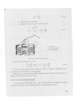
Fig. 1: Filling of a Mercury Thermometer
When the reservoir is heated, the mercury expands, rising through a long thin column,
upon which a graded ruler has been etched. What sort of sensitivity can be expected for
such a system?


Well, the thermal expansion coefficient of mercury is well known to be about 30 PPM/K.
If we assume that dimensions of the container do not change appreciably, (Is this a good
assumption?) then the mercury in the column expands linearly with temperature.

Therefore,

If we want 1 mm/K at room temperature, and we have a reservoir volume of 0.1 cm3, we
need:

Clearly, the sensitivity depends very strongly on the diameter of the column. Historically,
makers of thermometer tubes worked very hard to control column diameter.
Nevertheless, it was important to calibrate each thermometer with an ice point and a
boiling water reference.

Other traditional techniques for temperature measurement based on thermal expansion
are very popular even today. As we saw in the thermostat lab, a great many home
thermostats still rely on differential expansion in a bimorph to close a switch. Also,
toaster ovens that are a few years old still feature bimetal temperature switches to operate
the timing feature of the oven. Bimetal switches are fairly inexpensive, can operate
reliably for many cycles, and may still be the correct choice for temperature sensing
applications.
In many cases, bimetal temperature switches are not accurate enough, or do not allow
operation over a broad temperature range.
For high temperature applications, thermocouple thermometers are often used. The
thermocouple is an interesting device from a physics standpoint, but its operation can be
easily understood from a thermal model.
All metal wires may be considered as tubes filled with a fluid of electrons. The electrons
are more or less free to move about in the tube, and certainly move in a preferential
direction when a voltage is applied (voltage acts like a pressure). If the density of the
electrons is non-uniform, the non-uniform charge distribution exerts a force on the
electrons, tending to even them out. This charge effect is similar to a finite
compressibility in a normal fluid.


Now, suppose a tube filled with electrons is heated at one end. The effect of heat is to
increase the average thermal velocity (because 1/2 mv^2 is proportional to 1/2 kBT) of
the heated electrons. In this situation, the effect of heat is to increase the average velocity
of the electrons on the heated end of the wire. Because of this velocity increase, `warm'
electrons will leave the heated end of the wire faster than they can be replenished by
`cold' electrons from the other end. This will lead to a non-uniform density distribution
which gradually increases until the electrostatic pressure (because of the charges) is large
enough to balance it.
If one attached the leads of a voltmeter to this wire, there would be an excess of electrons
at the cold end, and a net voltage difference across the wire. Since the cold end has an

excess of electrons, it is repulsive to additional electrons, and is therefore at a `low'
voltage with respect to positive charges.
The amount of voltage difference is approximately proportional to temperature, and
depends on materials properties (e.g. electron mobility and thermal conductivity). Tables
of thermocouple properties are widely published.
Now, it is generally inconvenient to attach the leads of a voltmeter across the wire,
especially since one end is at the point of temperature measurement. Instead, it is
common to use a pair of wires made from 2 different materials. The wires are joined at
the end which is to be the point of temperature measurement (the `junction'), and the
voltage is measured across the other two ends. If the materials have different
thermocouple effects, there will be a voltage difference across those wires. Tables of the
thermocouple voltages for a set of standard pairs are also widely published. A good pair
of materials for a thermocouple are any materials which can each survive the
environment of the measurement, do not react with each other, and have suitable different
thermocouple coefficients.
The voltages generated by such effects are fairly small. A good thermocouple exhibits a
voltage signal of only 10 uV/Kelvin. Therefore, accurate measurements of small
temperature changes require very well-designed electronics. For measurements which
require accuracy of +/- 10 K, and need to be carried out at temperatures near 1000K,
thermocouples are definitely the way to go.
There are also many examples of thermometers based on resistance changes. We have
already seen several examples of resistance changes which are considered to be a
problem in measurements of other quantities (piezoresistive strain gauges, for example).


Fig. 2: RTD probes.
Platinum wires are commonly used for resistance thermometry. Even thought platinum is
quite expensive, it is favored for these applications for several very good reasons.
Do you know what they are?
For narrower temperature ranges, there are a large assortment of resistance thermometers.

ordinary carbon resistors can be used, but companies such as Thermometrics offer a
very broad collection of resistance thermometers in different shapes, sizes and
characteristics.
An important parameter for a resistance thermometer is the temperature coefficient,
generally denoted as Alpha. The temperature coefficient is defined as the fractional
change in resistance per unit change in temperature. This definition is convenient because
of the way it emerges from expressions which are associated with voltage divider-based
resistance measurement.


Fig. 3: NTC thermistor.


Fig. 4: PTC thermistor.
For a voltage divider with a thermistor of average resistance R1 and a load resistor with
resistance RL, the voltage at the output is given by

Now, if RL >> R1, we have

If the temperature of R1 changes by 1 K, the resistance changes by (Alpha R1), so the
voltage changes by Alpha(Vin R1/RL). The definition of the temperature coefficient as a


fractional change in resistance per unit change in temperature produces a result in which
the fractional change in voltage per unit change in temperature is given by alpha as well.
When using a thermistor to measure small temperature changes, noise can impose a
limitation. For example, all resistive elements exhibit voltage noise known as Johnson
noise with density given by

The resolution of a thermistor limited by Johnson noise would be given by:


We can see from this that the resolution is improved by reducing the temperature, the
bandwidth, and the load resistor, and by increasing the temperature coefficient and the
bias voltage, Vin. Of all of these parameters, it may be easiest to increase the bias voltage.
However, there is a problem to watch out for. The bias in this system also causes power
to be dissipated in the sense resistor. We may assume that the sense resistor is attached to
the object of interest with a finite thermal conductance G. There will be a temperature
difference between the sense resistor and the object of interest given by:

So, we can see that increasing the bias voltage can easily lead to problems. Since thermal
conductance between resistance thermometers and the surface are generally of order 10-2
to 1 W/K, we see that power dissipation in the mW range can cause substantial errors.
Because of this, manufacturers of resistance thermometers generally provide extensive
information on electrical measurement conditions to be used with their products.
Thermometrics, for instance, provides a lengthy (35 page) tutorial on their products in
their standard catalog.
In addition, there are a number of solid-state thermometer technologies which have
recently become commercially feasible. National Semiconductor, among other
companies, is marketing a family of thermometers based on diodes. The leakage current
in a forward-biased diode is generated by thermal excitation of electrons over an energy
barrier. At temperatures near room temperature, the voltage across a current-biased diode
is small and linearly dependent on temperature. National Semiconductor makes a series
of such devices which produce very nice voltage outputs over a decent range, and at low


cost. These devices look like 3-terminal transistors, require 5V and ground, and produce
an easily measured voltage output.
Finally, a number of commercially-available `non-contact' temperature sensors are
available which are based on measurement of infrared radiation. This approach can be
expensive, and can suffer from some calibration errors. The infrared radiation from any

object is given by:

For a room temperature object, this comes to 45 mW/cm2. This isn't much power, but is
easily detectable with a good sensor.
The difficulty lies in that the emissivity may be very difficult to know with any precision,
since it depends critically on surface finish, thin coatings of residue, and may depend on
temperature. Also, the radiation emitted by the object of interest may be absorbed by the
atmosphere. The atmosphere is reasonably transparent in some regions of the IR (3-5
microns, 8-12 microns), and basically opaque in others (6-7 microns, 14-20 microns).
Therefore, all of the radiation emitted by the surface cannot be expected to arrive at the
detector.
Finally, the radiation emitted by the surface is distributed more or less uniformly over the
entire field of view. Therefore, the amount available for detection is substantially less,
unless the instrument being used has a very large primary optical element.
All things considered, this is a difficult approach to use, and can be expensive. Good IR
detectors must be cooled, required an expensive package and operating system.
Nevertheless, these products are becoming popular for manufacturing applications, and
device and packaging costs can be expected to continue falling as the market grows...
For any thermometer, there are issues associated with measurement of changing
temperature that need to be considered. Consider a general situation in which a
thermometer is attached to an object with a thermal conductance of G (W/K). The
thermometer is a physical object, and has a heat capacity C (J/K). Assume that some
power, Pin, is being applied to the thermometer (bias currents?) Finally, assume that the
temperature of the object is oscillating in time according to:

where w is the frequency of oscillation. We assume that the temperature of the
thermometer is also oscillating, and that the frequencies are the same, so the temperature
of the thermometer may be expressed :



From energy balance, we know that the energy into the thermometer equals the change in
energy of the thermometer:

We can plug in our expressions for To and Ts, and we have:

We may separate the static and oscillating parts to give equations:

So, we should expect a finite temperature offset due to the bias power (P/G), and an
oscillation amplitude which varies with frequency. At low frequency, Ts2 is nearly equal
to To2, as we would hope for. At higher frequencies, the thermal time constant associated
with the heat capacity of the thermometer can cause a reduce oscillation and a phase lag.
These issues are important to keep in mind for measurements of time-varying
temperatures.
Parts after this may be repeated: We build a resistance measuring circuit in the form of a
voltage divider with a load resistor (RL) in series with the thermistor (Rs). As always, the
voltage at the output is given by

The resistance of the thermistor is

So,

Now, this is clearly a mess, and it is hard to see what the actual response function will
look like. To make some sense of it, we will do a Taylor series expansion of Vout(Rs) =


Vin Rs/(Rs + RL) about ∆T = 0, and extract the offset, the slope and the nonlinearity of this
response.
As mentioned in an earlier lecture, the Taylor series expansion is:

For our expression for Vout(Rs), we have:


Since Rs - Ro = Alpha Ro ∆T, we have

The sensitivity is defined as the derivative of the voltage with respect to the temperature
evaluated at ∆T = 0, so we have

The linearity of this system is essentially the maximum fractional error between the true
response and the linear response. A good approximation to this quantity may be
calculated by taking the ratio of the quadratic term in the expansion to the linear term.

which simplifies to:

We see that the linearity is improved (by reducing it) by taking RL>>Ro, and by keeping
either ∆T or Alpha small. Simply put, if we need a certain ∆T and a certain linearity, we
can select the thermometer Alpha and the load resistance to meet our needs.


When using a thermistor to measure small temperature changes, noise can impose a
limitation. For example, all resistive elements exhibit voltage noise known as Johnson
noise with density given by

The resolution of a thermistor limited by Johnson noise would be given by:

If we have made the simplifying assumption that RL>>Ro, we have

We can see from this that the resolution is improved by reducing the temperature, the
bandwidth, and the load resistor, and by increasing the temperature coefficient and the
bias voltage, Vin. Of all of these parameters, it may be easiest to increase the bias voltage.
However, increasing the bias voltage can cause heating problems.


Next some pictures considered in the development of these pages:


Fig. 5: Measuring the bore of a tube.

Fig. 6: Package of a thermometer.


Fig. 7: Thermometer probes.


Fig. 8: Size of a thermometer.

Fig. 9: Thermograph.