Tài liệu Image and Videl Comoression P5 pdf
Bạn đang xem bản rút gọn của tài liệu. Xem và tải ngay bản đầy đủ của tài liệu tại đây (586.32 KB, 23 trang )
5
© 2000 by CRC Press LLC
Variable-Length Coding:
Information Theory Results (II)
Recall the block diagram of encoders shown in Figure 2.3. There are three stages that take place
in an encoder: transformation, quantization, and codeword assignment. Quantization was discussed
in Chapter 2. Differential coding and transform coding using two different transformation compo-
nents were covered in Chapters 3 and 4, respectively. In differential coding it is the difference
signal that is quantized and encoded, while in transform coding it is the transformed signal that is
quantized and encoded. In this chapter and the next chapter, we discuss several codeword assignment
(encoding) techniques. In this chapter we cover two types of variable-length coding: Huffman
coding and arithmetic coding.
First we introduce some fundamental concepts of encoding. After that, the rules that must be
obeyed by all optimum and instantaneous codes are discussed. Based on these rules, the Huffman
coding algorithm is presented. A modified version of the Huffman coding algorithm is introduced as
an efficient way to dramatically reduce codebook memory while keeping almost the same optimality.
The promising arithmetic coding algorithm, which is quite different from Huffman coding, is
another focus of the chapter. While Huffman coding is a
block
-
oriented
coding technique, arithmetic
coding is a
stream
-
oriented
coding technique. With improvements in implementation, arithmetic
coding has gained increasing popularity. Both Huffman coding and arithmetic coding are included in
the international still image coding standard JPEG (Joint Photographic [image] Experts Group coding).
The adaptive arithmetic coding algorithms have been adopted by the international bilevel image coding
standard JBIG (Joint Bi-level Image experts Group coding). Note that the material presented in this
chapter can be viewed as a continuation of the information theory results presented in Chapter 1.
5.1 SOME FUNDAMENTAL RESULTS
Prior to presenting Huffman coding and arithmetic coding, we first provide some fundamental
concepts and results as necessary background.
5.1.1 C
ODING
AN
I
NFORMATION
S
OURCE
Consider an information source, represented by a
source alphabet S
.
(5.1)
where
s
i
, i
= 1,2,
L
,
m
are
source symbols.
Note that the terms source symbol and information
message are used interchangeably in the literature. In this book, however, we would like to
distinguish between them. That is, an information message can be a source symbol, or a combination
of source symbols. We denote
code alphabet
by
A
and
(5.2)
where
a
j
, j
= 1,2,
L
,
r
are
code symbols
. A
message code
is a sequence of code symbols that
represents a given information message. In the simplest case, a message consists of only a source
symbol. Encoding is then a procedure to assign a
codeword
to the source symbol. Namely,
Sss s
m
=
{}
12
,, ,L
Aaa a
r
=
{}
12
,,,L
© 2000 by CRC Press LLC
(5.3)
where the codeword
A
i
is a string of
k
code symbols assigned to the source symbol
s
i
. The term
message ensemble is defined as the entire set of messages. A code, also known as an ensemble
code, is defined as a mapping of all the possible sequences of symbols of
S
(message ensemble)
into the sequences of symbols in
A
.
Note that in binary coding, the number of code symbols
r
is equal to 2, since there are only
two code symbols available: the binary digits “0” and “1”. Two examples are given below to
illustrate the above concepts.
Example 5.1
Consider an English article and the ASCII code. Refer to Table 5.1. In this context, the source
alphabet consists of all the English letters in both lower and upper cases and all the punctuation
marks. The code alphabet consists of the binary 1 and 0. There are a total of 128 7-bit binary
codewords. From Table 5.1, we see that the codeword assigned to the capital letter A is 1000001.
That is, A is a source symbol, while 1000001 is its codeword.
Example 5.2
Table 5.2 lists what is known as the (5,2) code. It is a linear block code. In this example, the source
alphabet consists of the four (2
2
) source symbols listed in the left column of the table: 00, 01, 10,
and 11. The code alphabet consists of the binary 1 and 0. There are four codewords listed in the
right column of the table. From the table, we see that the code assigns a 5-bit codeword to each
source symbol. Specifically, the codeword of the source symbol 00 is 00000. The source symbol
01 is encoded as 10100; 01111 is the codeword assigned to 10. The symbol 11 is mapped to 11011.
5.1.2 S
OME
D
ESIRED
C
HARACTERISTICS
To be practical in use, codes need to have some desirable characteristics (Abramson, 1963). Some
of the characteristics are addressed in this subsection.
5.1.2.1 Block Code
A code is said to be a block code if it maps each source symbol in
S
into a fixed codeword in A.
Hence, the codes listed in the above two examples are block codes.
5.1.2.2 Uniquely Decodable Code
A code is uniquely decodable if it can be unambiguously decoded. Obviously, a code has to be
uniquely decodable if it is to be of use.
Example 5.3
Table 5.3 specifies a code. Obviously it is not uniquely decodable since if a binary string “00” is
received we do not know which of the following two source symbols has been sent out:
s
1
or
s
3
.
Nonsingular Code
A block code is nonsingular if all the codewords are distinct (see Table 5.4).
Example 5.4
Table 5.4 gives a nonsingular code since all four codewords are distinct. If a code is not a nonsingular
code, i.e., at least two codewords are identical, then the code is not uniquely decodable. Notice,
however, that a nonsingular code does not guarantee unique decodability. The code shown in
Table 5.4 is such an example in that it is nonsingular while it is not uniquely decodable. It is not
sAaa a
iiii
ik
Æ=
()
12
,,,L
© 2000 by CRC Press LLC
TABLE 5.1
Seven-Bit American Standard Code for Information Interchange (ASCII)
Bits
50 1 0 1 0 1 0 1
60 0 1 1 0 0 1 1
1 23470 0 0 0 1 1 1 1
0 0 0 0 NUL DLE SP 0 @ P ‘ p
1 0 0 0 SOH DC1 ! 1 A Q a q
0 1 0 0 STX DC2
≤
2BRb r
1 1 0 0 ETX DC3 # 3 C S c s
0 0 1 0 EOT DC4 $ 4 D T d t
1 0 1 0 ENQ NAK % 5 E U e u
0 110 ACK SYN & 6 F V f v
1 1 1 0 BEL ETB
¢
7GWg w
0 0 0 1 BS CAN ( 8 H X h x
1 0 0 1 HT EM ) 9 I Y i y
0 1 0 1 LF SUB * : J Z j z
1 1 0 1 VT ESC + ; K [ k {
0 0 1 1 FF FS , < L \ l |
1 0 1 1 CR GS - = M ] m }
0 1 1 1 SO RS . > N
Ÿ
n~
1 1 1 1 SI US / ? O
æ
o DEL
TABLE 5.2
A (5,2) Linear Block Code
Source Symbol Codeword
S
1
(0 0)
S
2
(0 1)
S
3
(1 0)
S
4
(1 1)
0 0 0 0 0
1 0 1 0 0
0 1 1 1 1
1 1 0 1 1
NUL Null, or all zeros DC1 Device control 1
SOH Start of heading DC2 Device control 2
STX Start of text DC3 Device control 3
ETX End of text DC4 Device control 4
EOT End of transmission NAK Negative acknowledgment
ENQ Enquiry SYN Synchronous idle
ACK Acknowledge ETB End of transmission block
BEL Bell, or alarm CAN Cancel
BS Backspace EM End of medium
HT Horizontal tabulation SUB Substitution
LF Line feed ESC Escape
VT Vertical tabulation FS File separator
FF Form feed GS Group separator
CR Carriage return RS Record separator
SO Shift out US Unit separator
SI Shift in SP Space
DLE Data link escape DEL Delete
© 2000 by CRC Press LLC
uniquely decodable because once the binary string “11” is received, we do not know if the source
symbols transmitted are
s
1
followed by
s
1
or simply
s
2
.
The
n
th Extension of a Block Code
The
n
th extension of a block code, which maps the source symbol
s
i
into the codeword
A
i
, is a
block code that maps the sequences of source symbols
s
i
1
s
i
2
L
s
in
into the sequences of codewords
A
i
1
A
i
2
L
A
in
.
A Necessary and Sufficient Condition of a Block Code’s Unique Decodability
A block code is uniquely decodable if and only if the
n
th extension of the code is nonsingular for
every finite
n
.
Example 5.5
The second extension of the nonsingular block code shown in Example 5.4 is listed in Table 5.5.
Clearly, this second extension of the code is not a nonsingular code, since the entries
s
1
s
2
and
s
2
s
1
are the same. This confirms the nonunique decodability of the nonsingular code in Example 5.4.
TABLE 5.3
A Not Uniquely Decodable Code
Source Symbol Codeword
S
1
S
2
S
3
S
4
0 0
1 0
0 0
1 1
TABLE 5.4
A Nonsingular Code
Source Symbol Codeword
S
1
S
2
S
3
S
4
1
1 1
0 0
0 1
TABLE 5.5
The Second Extension of the Nonsingular Block Code in
Example 5.4
Source Symbol Codeword Source Symbol Codeword
S
1
S
1
S
1
S
2
S
1
S
3
S
1
S
4
S
2
S
1
S
2
S
2
S
2
S
3
S
2
S
4
1 1
1 1 1
1 0 0
1 0 1
1 1 1
1 1 1 1
1 1 0 0
1 1 0 1
S
3
S
1
S
3
S
2
S
3
S
3
S
3
S
4
S
4
S
1
S
4
S
2
S
4
S
3
S
4
S
4
0 0 1
0 0 1 1
0 0 0 0
0 0 0 1
0 1 1
0 1 1 1
0 1 0 0
0 1 0 1
© 2000 by CRC Press LLC
5.1.2.3 Instantaneous Codes
Definition of Instantaneous Codes
A uniquely decodable code is said to be instantaneous if it is possible to decode each codeword
in a code symbol sequence without knowing the succeeding codewords.
Example 5.6
Table 5.6 lists three uniquely decodable codes. The first one is in fact a two-bit natural binary code.
In decoding, we can immediately tell which source symbols are transmitted since each codeword
has the same length. In the second code, code symbol “1” functions like a comma. Whenever we
see a “1”, we know it is the end of the codeword. The third code is different from the previous
two codes in that if we see a “10” string we are not sure if it corresponds to
s
2
until we see a
succeeding “1”. Specifically, if the next code symbol is “0”, we still cannot tell if it is
s
3
since the
next one may be “0” (hence
s
4
) or “1” (hence
s
3
). In this example, the next “1” belongs to the
succeeding codeword. Therefore we see that code 3 is uniquely decodable. It is not instantaneous,
however.
Definition of the
j
th Prefix
Assume a codeword
A
i
=
a
i
1
a
i
2
L
a
ik
. Then the sequences of code symbols
a
i
1
a
i
2
L
a
ij
with 1 £ j £ k
is the jth order prefix of the codeword A
i
.
Example 5.7
If a codeword is 11001, it has the following five prefixes: 11001, 1100, 110, 11, 1. The first-order
prefix is 1, while the fifth-order prefix is 11001.
A Necessary and Sufficient Condition of Being an Instantaneous Code
A code is instantaneous if and only if no codeword is a prefix of some other codeword. This
condition is often referred to as the prefix condition. Hence, the instantaneous code is also called
the prefix condition code or sometimes simply the prefix code. In many applications, we need a
block code that is nonsingular, uniquely decodable, and instantaneous.
5.1.2.4 Compact Code
A uniquely decodable code is said to be compact if its average length is the minimum among all
other uniquely decodable codes based on the same source alphabet S and code alphabet A. A
compact code is also referred to as a minimum redundancy code, or an optimum code.
Note that the average length of a code was defined in Chapter 1 and is restated below.
5.1.3 DISCRETE MEMORYLESS SOURCES
This is the simplest model of an information source. In this model, the symbols generated by the
source are independent of each other. That is, the source is memoryless or it has a zero memory.
Consider the information source expressed in Equation 5.1 as a discrete memoryless source.
The occurrence probabilities of the source symbols can be denoted by p(s
1
), p(s
2
), L, p(s
m
). The
TABLE 5.6
Three Uniquely Decodable Codes
Source Symbol Code 1 Code 2 Code 3
S
1
S
2
S
3
S
4
0 0
0 1
1 0
1 1
1
0 1
0 0 1
0 0 0 1
1
10
1 0 0
1 0 0 0
© 2000 by CRC Press LLC
lengths of the codewords can be denoted by l
1
, l
2
, L, l
m
. The average length of the code is then
equal to
(5.4)
Recall Shannon’s first theorem, i.e., the noiseless coding theorem described in Chapter 1. The
average length of the code is bounded below by the entropy of the information source. The entropy
of the source S is defined as H(S) and
(5.5)
Recall that entropy is the average amount of information contained in a source symbol. In
Chapter 1 the efficiency of a code, h, is defined as the ratio between the entropy and the average
length of the code. That is, h = H(S)/L
avg
. The redundancy of the code, z, is defined as z = 1 – h.
5.1.4 EXTENSIONS OF A DISCRETE MEMORYLESS SOURCE
Instead of coding each source symbol in a discrete source alphabet, it is often useful to code blocks
of symbols. It is, therefore, necessary to define the nth extension of a discrete memoryless source.
5.1.4.1 Definition
Consider the zero-memory source alphabet S defined in Equation 5.1. That is, S = {s
1
, s
2
, L, s
m
}.
If n symbols are grouped into a block, then there is a total of m
n
blocks. Each block is considered
as a new source symbol. These m
n
blocks thus form an information source alphabet, called the nth
extension of the source S, which is denoted by S
n
.
5.1.4.2 Entropy
Let each block be denoted by b
i
and
(5.6)
Then we have the following relation due to the memoryless assumption:
(5.7)
Hence, the relationship between the entropy of the source S and the entropy of its nth extension is
as follows:
(5.8)
Example 5.8
Table 5.7 lists a source alphabet. Its second extension is listed in Table 5.8.
Llps
avg i i
i
m
=
()
=
Â
1
HS ps ps
ii
i
m
()
=-
() ()
=
Â
log
2
1
b
iii in
ss s=
()
12
,,,L
pps
iij
j
n
b
()
=
()
=
’
1
HS n HS
n
()
=◊
()
© 2000 by CRC Press LLC
The entropy of the source and its second extension are calculated below.
It is seen that H(S
2
) = 2H(S).
5.1.4.3 Noiseless Source Coding Theorem
The noiseless source coding theorem, also known as Shannon’s first theorem, defining the minimum
average codeword length per source pixel, was presented in Chapter 1, but without a mathematical
expression. Here, we provide some mathematical expressions in order to give more insight about
the theorem.
For a discrete zero-memory information source S, the noiseless coding theorem can be expressed
as
(5.9)
That is, there exists a variable-length code whose average length is bounded below by the entropy
of the source (that is encoded) and bounded above by the entropy plus 1. Since the nth extension
of the source alphabet, S
n
, is itself a discrete memoryless source, we can apply the above result to
it. That is,
(5.10)
where L
n
avg
is the average codeword length of a variable-length code for the S
n
. Since H(S
n
) = nH(S)
and L
n
avg
= nL
n
avg, we have
(5.11)
TABLE 5.7
A Discrete Memoryless Source Alphabet
Source Symbol Occurrence Probability
S
1
S
2
0.6
0.4
TABLE 5.8
The Second Extension of the Source
Alphabet Shown in Table 5.7
Source Symbol Occurrence Probability
S
1
S
1
S
2
S
2
S
2
S
1
S
2
S
2
0.36
0.24
0.24
0.16
HS
HS
()
=- ◊
()
-◊
()
ª
()
=- ◊
()
-◊ ◊
()
-◊
()
ª
06 06 04 04 097
0 36 0 36 2 0 24 0 24 0 16 0 16 1 94
22
2
222
. log . . log . .
. log . . log . . log . .
HS L HS
avg
()
£<
()
+ 1
HS L HS
n
avg
nn
()
£<
()
+ 1
HS L HS
n
avg
()
£<
()
+
1
© 2000 by CRC Press LLC
Therefore, when coding blocks of n source symbols, the noiseless source coding theory states that
for an arbitrary positive number e, there is a variable-length code which satisfies the following:
(5.12)
as n is large enough. That is, the average number of bits used in coding per source symbol is
bounded below by the entropy of the source and is bounded above by the sum of the entropy and
an arbitrary positive number. To make e arbitrarily small, i.e., to make the average length of the
code arbitrarily close to the entropy, we have to make the block size n large enough. This version
of the noiseless coding theorem suggests a way to make the average length of a variable-length
code approach the source entropy. It is known, however, that the high coding complexity that occurs
when n approaches infinity makes implementation of the code impractical.
5.2 HUFFMAN CODES
Consider the source alphabet defined in Equation 5.1. The method of encoding source symbols
according to their probabilities, suggested in (Shannon, 1948; Fano, 1949), is not optimum. It
approaches the optimum, however, when the block size n approaches infinity. This results in a large
storage requirement and high computational complexity. In many cases, we need a direct encoding
method that is optimum and instantaneous (hence uniquely decodable) for an information source
with finite source symbols in source alphabet S. Huffman code is the first such optimum code
(Huffman, 1952), and is the technique most frequently used at present. It can be used for r-ary
encoding as r > 2. For notational brevity, however, we discuss only the Huffman coding used in
the binary case presented here.
5.2.1 REQUIRED RULES FOR OPTIMUM INSTANTANEOUS CODES
Let us rewrite Equation 5.1 as follows:
(5.13)
Without loss of generality, assume the occurrence probabilities of the source symbols are as
follows:
(5.14)
Since we are seeking the optimum code for S, the lengths of codewords assigned to the source
symbols should be
(5.15)
Based on the requirements of the optimum and instantaneous code, Huffman derived the
following rules (restrictions):
1. (5.16)
Equations 5.14 and 5.16 imply that when the source symbol occurrence probabilities are
arranged in a nonincreasing order, the length of the corresponding codewords should be
in a nondecreasing order. In other words, the codeword length of a more probable source
HS L HS
avg
()
£<
()
+e
Sss s
m
=
()
12
,, ,L
ps ps ps ps
mm12 1
()
≥
()
≥≥
()
≥
()
-
L
ll l l
mm12 1
££ £ £
-
L .
ll l l
mm12 1
££ £ =
-
L
© 2000 by CRC Press LLC
symbol should not be longer than that of a less probable source symbol. Furthermore,
the length of the codewords assigned to the two least probable source symbols should
be the same.
2. The codewords of the two least probable source symbols should be the same except for
their last bits.
3. Each possible sequence of length l
m
– 1 bits must be used either as a codeword or must
have one of its prefixes used as a codeword.
Rule 1 can be justified as follows. If the first part of the rule, i.e., l
1
£ l
2
£ L £ l
m–1
is violated,
say, l
1
> l
2
, then we can exchange the two codewords to shorten the average length of the code.
This means the code is not optimum, which contradicts the assumption that the code is optimum.
Hence it is impossible. That is, the first part of Rule 1 has to be the case. Now assume that the
second part of the rule is violated, i.e., l
m–1
< l
m
. (Note that l
m–1
> l
m
can be shown to be impossible
by using the same reasoning we just used in proving the first part of the rule.) Since the code is
instantaneous, codeword A
m–1
is not a prefix of codeword A
m
. This implies that the last bit in the
codeword A
m
is redundant. It can be removed to reduce the average length of the code, implying
that the code is not optimum. This contradicts the assumption, thus proving Rule 1.
Rule 2 can be justified as follows. As in the above, A
m–1
and A
m
are the codewords of the two
least probable source symbols. Assume that they do not have the identical prefix of the order l
m
– 1.
Since the code is optimum and instantaneous, codewords A
m–1
and A
m
cannot have prefixes of any
order that are identical to other codewords. This implies that we can drop the last bits of A
m–1
and
A
m
to achieve a lower average length. This contradicts the optimum code assumption. It proves that
Rule 2 has to be the case.
Rule 3 can be justified using a similar strategy to that used above. If a possible sequence of
length l
m
– 1 has not been used as a codeword and any of its prefixes have not been used as
codewords, then it can be used in place of the codeword of the mth source symbol, resulting in a
reduction of the average length L
avg
. This is a contradiction to the optimum code assumption and
it justifies the rule.
5.2.2 HUFFMAN CODING ALGORITHM
Based on these three rules, we see that the two least probable source symbols have codewords of
equal length. These two codewords are identical except for the last bits, the binary 0 and 1,
respectively. Therefore, these two source symbols can be combined to form a single new symbol.
Its occurrence probability is the sum of two source symbols, i.e., p(s
m–1
) + p(s
m
). Its codeword is
the common prefix of order l
m
– 1 of the two codewords assigned to s
m
and s
m–1
, respectively. The
new set of source symbols thus generated is referred to as the first auxiliary source alphabet, which
is one source symbol less than the original source alphabet. In the first auxiliary source alphabet,
we can rearrange the source symbols according to a nonincreasing order of their occurrence
probabilities. The same procedure can be applied to this newly created source alphabet. A binary
0 and a binary 1, respectively, are assigned to the last bits of the two least probable source symbols
in the alphabet. The second auxiliary source alphabet will again have one source symbol less than
the first auxiliary source alphabet. The procedure continues. In some step, the resultant source
alphabet will have only two source symbols. At this time, we combine them to form a single source
symbol with a probability of 1. The coding is then complete.
Let’s go through the following example to illustrate the above Huffman algorithm.
Example 5.9
Consider a source alphabet whose six source symbols and their occurrence probabilities are listed
in Table 5.9. Figure 5.1 demonstrates the Huffman coding procedure applied. In the example, among
the two least probable source symbols encountered at each step we assign binary 0 to the top
symbol and binary 1 to the bottom symbol.
© 2000 by CRC Press LLC
5.2.2.1 Procedures
In summary, the Huffman coding algorithm consists of the following steps.
1. Arrange all source symbols in such a way that their occurrence probabilities are in a
nonincreasing order.
2. Combine the two least probable source symbols:
• Form a new source symbol with a probability equal to the sum of the probabilities
of the two least probable symbols.
• Assign a binary 0 and a binary 1 to the two least probable symbols.
3. Repeat until the newly created auxiliary source alphabet contains only one source symbol.
4. Start from the source symbol in the last auxiliary source alphabet and trace back to each
source symbol in the original source alphabet to find the corresponding codewords.
5.2.2.2 Comments
First, it is noted that the assignment of the binary 0 and 1 to the two least probable source symbols
in the original source alphabet and each of the first (u – 1) auxiliary source alphabets can be
implemented in two different ways. Here u denotes the total number of the auxiliary source symbols
in the procedure. Hence, there is a total of 2
u
possible Huffman codes. In Example 5.9, there are
five auxiliary source alphabets, hence a total of 2
5
= 32 different codes. Note that each is optimum:
that is, each has the same average length.
Second, in sorting the source symbols, there may be more than one symbol having equal
probabilities. This results in multiple arrangements of symbols, hence multiple Huffman codes.
While all of these Huffman codes are optimum, they may have some other different properties.
TABLE 5.9
Source Alphabet and Huffman Codes in Example 5.9
Source Symbol Occurrence Probability Codeword Assigned Length of Codeword
S
1
S
2
S
3
S
4
S
5
S
6
0.3
0.1
0.2
0.05
0.1
0.25
00
101
11
1001
1000
01
2
3
2
4
4
2
FIGURE 5.1 Huffman coding procedure in Example 5.9.
© 2000 by CRC Press LLC
For instance, some Huffman codes result in the minimum codeword length variance (Sayood, 1996).
This property is desired for applications in which a constant bit rate is required.
Third, Huffman coding can be applied to r-ary encoding with r > 2. That is, code symbols are
r-ary with r > 2.
5.2.2.3 Applications
As a systematic procedure to encode a finite discrete memoryless source, the Huffman code has
found wide application in image and video coding. Recall that it has been used in differential
coding and transform coding. In transform coding, as introduced in Chapter 4, the magnitude of
the quantized transform coefficients and the run-length of zeros in the zigzag scan are encoded by
using the Huffman code. This has been adopted by both still image and video coding standards.
5.3 MODIFIED HUFFMAN CODES
5.3.1 M
OTIVATION
As a result of Huffman coding, a set of all the codewords, called a codebook, is created. It is an
agreement between the transmitter and the receiver. Consider the case where the occurrence
probabilities are skewed, i.e., some are large, while some are small. Under these circumstances,
the improbable source symbols take a disproportionately large amount of memory space in the
codebook. The size of the codebook will be very large if the number of the improbable source
symbols is large. A large codebook requires a large memory space and increases the computational
complexity. A modified Huffman procedure was therefore devised in order to reduce the memory
requirement while keeping almost the same optimality (Hankamer, 1979).
Example 5.10
Consider a source alphabet consisting of 16 symbols, each being a 4-bit binary sequence. That is,
S = {s
i
, i = 1,2,L,16}. The occurrence probabilities are
The source entropy can be calculated as follows:
Applying the Huffman coding algorithm, we find that the codeword lengths associated with
the symbols are: l
1
= l
2
= 2, l
3
= 4, and l
4
= l
5
= L = l
16
= 5, where l
i
denotes the length of the ith
codeword. The average length of Huffman code is
We see that the average length of Huffman code is quite close to the lower entropy bound. It is
noted, however, that the required codebook memory, M (defined as the sum of the codeword lengths),
is quite large:
ps ps
ps ps ps
12
34
16
14
128
()
=
()
=
()
=
()
==
()
=
,
.L
H S ymbol
()
=◊-
Ê
Ë
ˆ
¯
+◊-
Ê
Ë
ˆ
¯
ª2
1
4
1
4
14
1
28
1
28
3 404
22
log log . bits per s
Lpsl
avg i i
i
=
()
=
=
Â
3 464
1
16
. bits per symbol
© 2000 by CRC Press LLC
This number is obviously larger than the average codeword length multiplied by the number of
codewords. This should not come as a surprise since the average here is in the statistical sense instead
of in the arithmetic sense. When the total number of improbable symbols increases, the required
codebook memory space will increase dramatically, resulting in a great demand on memory space.
5.3.2 ALGORITHM
Consider a source alphabet S that consists of 2
v
binary sequences, each of length v. In other words,
each source symbol is a v-bit codeword in the natural binary code. The occurrence probabilities
are highly skewed and there is a large number of improbable symbols in S. The modified Huffman
coding algorithm is based on the following idea: lumping all the improbable source symbols into
a category named ELSE (Weaver, 1978). The algorithm is described below.
1. Categorize the source alphabet S into two disjoint groups, S
1
and S
2
, such that
(5.17)
and
(5.18)
2. Establish a source symbol ELSE with its occurrence probability equal to p(S
2
).
3. Apply the Huffman coding algorithm to the source alphabet S
3
with S
3
= S
1
U ELSE.
4. Convert the codebook of S
3
to that of S as follows.
• Keep the same codewords for those symbols in S
1
.
• Use the codeword assigned to ELSE as a prefix for those symbols in S
2
.
5.3.3 CODEBOOK MEMORY REQUIREMENT
Codebook memory M is the sum of the codeword lengths. The M required by Huffman coding
with respect to the original source alphabet S is
(5.19)
where l
i
denotes the length of the ith codeword, as defined previously. In the case of the modified
Huffman coding algorithm, the memory required M
mH
is
(5.20)
where l
ELSE
is the length of the codeword assigned to ELSE. The above equation reveals the big
savings in memory requirement when the probability is skewed. The following example is used to
illustrate the modified Huffman coding algorithm and the resulting dramatic memory savings.
M l bits
i
i
==
=
Â
73
1
16
Ssps
ii
v
1
1
2
=
()
>
Ï
Ì
Ó
¸
˝
˛
Ssps
ii
v
2
1
2
=
()
£
Ï
Ì
Ó
¸
˝
˛
Ml ll
i
iS
i
iS
i
iS
==+
ŒŒŒ
ÂÂÂ
12
Mlll
mH i
iS
i
iS
ELSE
==+
ŒŒ
ÂÂ
31
© 2000 by CRC Press LLC
Example 5.11
In this example, we apply the modified Huffman coding algorithm to the source alphabet presented
in Example 5.10. We first lump the 14 symbols having the least occurrence probabilities together
to form a new symbol ELSE. The probability of ELSE is the sum of the 14 probabilities. That is,
p(ELSE) = · 14 = .
Apply Huffman coding to the new source alphabet S
3
= {s
1
, s
2
, ELSE}, as shown in Figure 5.2.
From Figure 5.2, it is seen that the codewords assigned to symbols s
1
, s
2
, and ELSE, respectively,
are 10, 11, and 0. Hence, for every source symbol lumped into ELSE, its codeword is 0 followed
by the original 4-bit binary sequence. Therefore, M
mH
= 2 + 2 + 1 = 5 bits, i.e., the required
codebook memory is only 5 bits. Compared with 73 bits required by Huffman coding (refer to
Example 5.10), there is a savings of 68 bits in codebook memory space. Similar to the comment
made in Example 5.10, the memory savings will be even larger if the probability distribution is
skewed more severely and the number of improbable symbols is larger. The average length of the
modified Huffman algorithm is . This demonstrates
that modified Huffman coding retains almost the same coding efficiency as that achieved by
Huffman coding.
5.3.4 BOUNDS ON AVERAGE CODEWORD LENGTH
It has been shown that the average length of the modified Huffman codes satisfies the following
condition:
(5.21)
where p = S
s
i
Πs
2
p(s
i
). It is seen that, compared with the noiseless source coding theorem, the upper
bound of the code average length is increased by a quantity of –p log
2
p. In Example 5.11 it is
seen that the average length of the modified Huffman code is close to that achieved by the Huffman
code. Hence the modified Huffman code is almost optimum.
5.4 ARITHMETIC CODES
Arithmetic coding, which is quite different from Huffman coding, is gaining increasing popularity.
In this section, we will first analyze the limitations of Huffman coding. Then the principle of
arithmetic coding will be introduced. Finally some implementation issues are discussed briefly.
FIGURE 5.2 The modified Huffman coding procedure in Example 5.11.
1
28
1
2
L
avg mH,
. =◊◊+ ◊◊ =
1
4
1
28
22 514 35bits per symbo
l
HS L HS p p
avg
()
£<
()
+-1
2
log
© 2000 by CRC Press LLC
5.4.1 LIMITATIONS OF HUFFMAN CODING
As seen in Section 5.2, Huffman coding is a systematic procedure for encoding a source alphabet,
with each source symbol having an occurrence probability. Under these circumstances, Huffman
coding is optimum in the sense that it produces a minimum coding redundancy. It has been shown
that the average codeword length achieved by Huffman coding satisfies the following inequality
(Gallagher, 1978).
(5.22)
where H(S) is the entropy of the source alphabet, and p
max
denotes the maximum occurrence
probability in the set of the source symbols. This inequality implies that the upper bound of the
average codeword length of Huffman code is determined by the entropy and the maximum occur-
rence probability of the source symbols being encoded.
In the case where the probability distribution among source symbols is skewed (some proba-
bilities are small, while some are quite large), the upper bound may be large, implying that the
coding redundancy may not be small. Imagine the following extreme situation. There are only two
source symbols. One has a very small probability, while the other has a very large probability (very
close to 1). The entropy of the source alphabet in this case is close to 0 since the uncertainty is
very small. Using Huffman coding, however, we need two bits: one for each. That is, the average
codeword length is 1, which means that the redundancy is very close to 1. This agrees with
Equation 5.22. This inefficiency is due to the fact that Huffman coding always encodes a source
symbol with an integer number of bits.
The noiseless coding theorem (reviewed in Section 5.1) indicates that the average codeword
length of a block code can approach the source alphabet entropy when the block size approaches
infinity. As the block size approaches infinity, the storage required, the codebook size, and the
coding delay will approach infinity, however, and the complexity of the coding will be out of control.
The fundamental idea behind Huffman coding and Shannon-Fano coding (devised a little earlier
than Huffman coding [Bell et al., 1990]) is block coding. That is, some codeword having an integral
number of bits is assigned to a source symbol. A message may be encoded by cascading the relevant
codewords. It is the block-based approach that is responsible for the limitations of Huffman codes.
Another limitation is that when encoding a message that consists of a sequence of source
symbols, the nth extension Huffman coding needs to enumerate all possible sequences of source
symbols having the same length, as discussed in coding the nth extended source alphabet. This is
not computationally efficient.
Quite different from Huffman coding, arithmetic coding is stream-based. It overcomes the
drawbacks of Huffman coding. A string of source symbols is encoded as a string of code symbols.
Hence, it is free of the integral-bits-per-source symbol restriction and is more efficient. Arithmetic
coding may reach the theoretical bound to coding efficiency specified in the noiseless source coding
theorem for any information source. Below, we introduce the principle of arithmetic coding, from
which we can see the stream-based nature of arithmetic coding.
5.4.2 PRINCIPLE OF ARITHMETIC CODING
To understand the different natures of Huffman coding and arithmetic coding, let us look at
Example 5.12, where we use the same source alphabet and the associated occurrence probabilities
used in Example 5.9. In this example, however, a string of source symbols s
1
s
2
s
3
s
4
s
5
s
6
is encoded.
Note that we consider the terms string and stream to be slightly different. By stream, we mean a
message, or possibly several messages, which may correspond to quite a long sequence of source
symbols. Moreover, stream gives a dynamic “flavor.” Later on we will see that arithmetic coding
HS L HS p
avg
()
£<
()
++
max
.0 086
© 2000 by CRC Press LLC
is implemented in an incremental manner. Hence stream is a suitable term to use for arithmetic
coding. In this example, however, only six source symbols are involved. Hence we consider the
term string to be suitable, aiming at distinguishing it from the term block.
Example 5.12
The set of six source symbols and their occurrence probabilities are listed in Table 5.10. In this
example, the string to be encoded using arithmetic coding is s
1
s
2
s
3
s
4
s
5
s
6
. In the following four
subsections we will use this example to illustrate the principle of arithmetic coding and decoding.
5.4.2.1 Dividing Interval [0,1) into Subintervals
As pointed out by Elias, it is not necessary to sort out source symbols according to their occurrence
probabilities. Therefore in Figure 5.3(a) the six symbols are arranged in their natural order, from
symbols s
1
, s
2
, L, up to s
6
. The real interval between 0 and 1 is divided into six subintervals, each
having a length of p(s
i
), i = 1,2,L,6. Specifically, the interval denoted by [0,1) — where 0 is
included in (the left end is closed) and 1 is excluded from (the right end is open) the interval —
is divided into six subintervals. The first subinterval [0, 0.3) corresponds to s
1
and has a length of
P(s
1
), i.e., 0.3. Similarly, the subinterval [0, 0.3) is said to be closed on the left and open on the
right. The remaining five subintervals are similarly constructed. All six subintervals thus formed
are disjoint and their union is equal to the interval [0, 1). This is because the sum of all the
probabilities is equal to 1.
We list the sum of the preceding probabilities, known as cumulative probability (Langdon,
1984), in the right-most column of Table 5.10 as well. Note that the concept of cumulative prob-
ability (CP) is slightly different from that of cumulative distribution function (CDF) in probability
theory. Recall that in the case of discrete random variables the CDF is defined as follows.
(5.23)
The CP is defined as
(5.24)
where CP(s
1
) = 0 is defined. Now we see each subinterval has its lower end point located at CP(s
i
).
The width of each subinterval is equal to the probability of the corresponding source symbol. A
subinterval can be completely defined by its lower end point and its width. Alternatively, it is
TABLE 5.10
Source Alphabet and Cumulative Probabilities in Example 5.12
Source Symbol Occurrence Probability Associated Subintervals CP
S
1
S
2
S
3
S
4
S
5
S
6
0.3
0.1
0.2
0.05
0.1
0.25
[0, 0.3)
[0.3, 0.4)
[0.4, 0.6)
[0.6, 0.65)
[0.65, 0.75)
[0.75, 1.0)
0
0.3
0.4
0.6
0.65
0.75
CDF s p s
ij
j
i
()
=
()
=
Â
1
CP s p s
ij
j
i
()
=
()
=
-
Â
1
1
© 2000 by CRC Press LLC
determined by its two end points: the lower and upper end points (sometimes also called the left
and right end points).
Now we consider encoding the string of source symbols s
1
s
2
s
3
s
4
s
5
s
6
with the arithmetic coding
method.
5.4.2.2 Encoding
Encoding the First Source Symbol
Refer to Figure 5.3(a). Since the first symbol is s
1
, we pick up its subinterval [0, 0.3). Picking up
the subinterval [0, 0.3) means that any real number in the subinterval, i.e., any real number equal
to or greater than 0 and smaller than 0.3, can be a pointer to the subinterval, thus representing the
source symbol s
1
. This can be justified by considering that all the six subintervals are disjoint.
Encoding the Second Source Symbol
Refer to Figure 5.3(b). We use the same procedure as used in part (a) to divide the interval [0, 0.3)
into six subintervals. Since the second symbol to be encoded is s
2
, we pick up its subinterval [0.09,
0.12).
FIGURE 5.3 Arithmetic coding working on the same source alphabet as that in Example 5.9. The encoded
symbol string is S
1
S
2
S
3
S
4
S
5
S
6
.
© 2000 by CRC Press LLC
Notice that the subintervals are recursively generated from part (a) to part (b). It is known that
an interval may be completely specified by its lower end point and width. Hence, the subinterval
recursion in the arithmetic coding procedure is equivalent to the following two recursions: end
point recursion and width recursion.
From interval [0, 0.3) derived in part (a) to interval [0.09, 0.12) obtained in part (b), we can
conclude the following lower end point recursion:
(5.25)
where L
new
, L
current
represent, respectively, the lower end points of the new and current recursions,
and the W
current
and the CP
new
denote, respectively, the width of the interval in the current recursion
and the cumulative probability in the new recursion. The width recursion is
(5.26)
where W
new
, and p(s
i
) are, respectively, the width of the new subinterval and the probability of the
source symbol s
i
that is being encoded. These two recursions, also called double recursion (Langdon,
1984), play a central role in arithmetic coding.
Encoding the Third Source Symbol
Refer to Figure 5.3(c). When the third source symbol is encoded, the subinterval generated above
in part (b) is similarly divided into six subintervals. Since the third symbol to encode is s
3
, its
subinterval [0.102, 0.108) is picked up.
Encoding the Fourth, Fifth, and Sixth Source Symbols
Refer to Figure 5.3(d,e,f). The subinterval division is carried out according to Equations 5.25 and
5.26. The symbols s
4
, s
5
, and s
6
are encoded. The final subinterval generated is [0.1058175,
0.1058250).
That is, the resulting subinterval [0.1058175, 0.1058250) can represent the source symbol string
s
1
s
2
s
3
s
4
s
5
s
6
. Note that in this example decimal digits instead of binary digits are used. In binary
arithmetic coding, the binary digits 0 and 1 are used.
5.4.2.3 Decoding
As seen in this example, for the encoder of arithmetic coding, the input is a source symbol string
and the output is a subinterval. Let us call this the final subinterval or the resultant subinterval.
Theoretically, any real numbers in the interval can be the code string for the input symbol string
since all subintervals are disjoint. Often, however, the lower end of the final subinterval is used as
the code string. Now let us examine how the decoding process is carried out with the lower end
of the final subinterval.
Decoding sort of reverses what encoding has done. The decoder knows the encoding procedure
and therefore has the information contained in Figure 5.3(a). It compares the lower end point of
the final subinterval 0.1058175 with all the end points in (a). It is determined that 0 < 0.1058175 <
0.3. That is, the lower end falls into the subinterval associated with the symbol s
1
. Therefore, the
symbol s
1
is first decoded.
Once the first symbol is decoded, the decoder may know the partition of subintervals shown in
Figure 5.3(b). It is then determined that 0.09 < 0.1058175 < 0.12. That is, the lower end is contained
in the subinterval corresponding to the symbol s
2
. As a result, s
2
is the second decoded symbol.
The procedure repeats itself until all six symbols are decoded. That is, based on Figure 5.3(c),
it is found that 0.102 < 0.1058175 < 0.108. The symbol s
3
is decoded. Then, the symbols s
4
, s
5
, s
6
are subsequently decoded because the following inequalities are determined:
LL W CP
new current current new
=+◊
WW ps
new current i
=◊
()
© 2000 by CRC Press LLC
0.1056 < 0.1058175 < 0.1059
0.105795 < 0.1058175 < 0.1058250
0.1058145 < 0.1058175 < 0.1058250
Note that a terminal symbol is necessary to inform the decoder to stop decoding.
The above procedure gives us an idea of how decoding works. The decoding process, however,
does not need to construct parts (b), (c), (d), (e), and (f) of Figure 5.3. Instead, the decoder only
needs the information contained in Figure 5.3(a). Decoding can be split into the following three
steps: comparison, readjustment (subtraction), and scaling (Langdon, 1984).
As described above, through comparison we decode the first symbol s
1
. From the way
Figure 5.3(b) is constructed, we know the decoding of s
2
can be accomplished as follows. We
subtract the lower end of the subinterval associated with s
1
in part (a), that is, 0 in this example,
from the lower end of the final subinterval 0.1058175, resulting in 0.1058175. Then we divide this
number by the width of the subinterval associated with s
1
, i.e., the probability of s
1
, 0.3, resulting
in 0.352725. Looking at part (a) of Figure 5.3, it is found that 0.3 < 0.352725 < 0.4. That is, the
number is within the subinterval corresponding to s
2
. Therefore the second decoded symbol is s
2
.
Note that these three decoding steps exactly “undo” what encoding did.
To decode the third symbol, we subtract the lower end of the subinterval with s
2
, 0.3 from
0.352725, obtaining 0.052725. This number is divided by the probability of s
2
, 0.1, resulting in
0.52725. The comparison of 0.52725 with end points in part (a) reveals that the third decoded
symbol is s
3
.
In decoding the fourth symbol, we first subtract the lower end of the s
3
’s subinterval in part (a),
0.4 from 0.52725, getting 0.12725. Dividing 0.12725 by the probability of s
3
, 0.2, results in 0.63625.
Referring to part (a), we decode the fourth symbol as s
4
by comparison.
Subtraction of the lower end of the subinterval of s
4
in part (a), 0.6, from 0.63625 leads to
0.03625. Division of 0.03625 by the probability of s
4
, 0.05, produces 0.725. The comparison
between 0.725 and the end points in part (a) decodes the fifth symbol as s
5
.
Subtracting 0.725 by the lower end of the subinterval associated with s
5
in part (a), 0.65, gives
0.075. Dividing 0.075 by the probability of s
5
, 0.1, generates 0.75. The comparison indicates that
the sixth decoded symbol is s
6
.
In summary, considering the way in which parts (b), (c), (d), (e), and (f) of Figure 5.3 are
constructed, we see that the three steps discussed in the decoding process: comparison, readjustment,
and scaling, exactly “undo” what the encoding procedure has done.
5.4.2.4 Observations
Both encoding and decoding involve only arithmetic operations (addition and multiplication in
encoding, subtraction and division in decoding). This explains the name arithmetic coding.
We see that an input source symbol string s
1
s
2
s
3
s
4
s
5
s
6
, via encoding, corresponds to a subinterval
[0.1058175, 0.1058250). Any number in this interval can be used to denote the string of the source
symbols.
We also observe that arithmetic coding can be carried out in an incremental manner. That is,
source symbols are fed into the encoder one by one and the final subinterval is refined continually,
i.e., the code string is generated continually. Furthermore, it is done in a manner called first in first
out (FIFO). That is, the source symbol encoded first is decoded first. This manner is superior to
that of last in first out (LIFO). This is because FIFO is suitable for adaptation to the statistics of
the symbol string.
It is obvious that the width of the final subinterval becomes smaller and smaller when the length
of the source symbol string becomes larger and larger. This causes what is known as the precision
© 2000 by CRC Press LLC
problem. It is this problem that prohibited arithmetic coding from practical usage for quite a long
period of time. Only after this problem was solved in the late 1970s, did arithmetic coding become
an increasingly important coding technique.
It is necessary to have a termination symbol at the end of an input source symbol string. In
this way, an arithmetic coding system is able to know when to terminate decoding.
Compared with Huffman coding, arithmetic coding is quite different. Basically, Huffman coding
converts each source symbol into a fixed codeword with an integral number of bits, while arithmetic
coding converts a source symbol string to a code symbol string. To encode the same source symbol
string, Huffman coding can be implemented in two different ways. One way is shown in Example 5.9.
We construct a fixed codeword for each source symbol. Since Huffman coding is instantaneous,
we can cascade the corresponding codewords to form the output, a 17-bit code string
00.101.11.1001.1000.01, where, for easy reading, the five periods are used to indicate different
codewords. As we see that for the same source symbol string, the final subinterval obtained by
using arithmetic coding is [0.1058175, 0.1058250). It is noted that a decimal in binary number
system, 0.000110111111111, which is of 15 bits, is equal to the decimal in decimal number system,
0.1058211962, which falls into the final subinterval representing the string s
1
s
2
s
3
s
4
s
5
s
6
. This indi-
cates that, for this example, arithmetic coding is more efficient than Huffman coding.
Another way is to form a sixth extension of the source alphabet as discussed in Section 5.1.4:
treat each group of six source symbols as a new source symbol; calculate its occurrence probability
by multiplying the related six probabilities; then apply the Huffman coding algorithm to the sixth
extension of the discrete memoryless source. This is called the sixth extension of Huffman block
code (refer to Section 5.1.2.2). In other words, in order to encode the source string s
1
s
2
s
3
s
4
s
5
s
6
,
Huffman coding encodes all of the 6
6
= 46,656 codewords in the sixth extension of the source
alphabet. This implies a high complexity in implementation and a large codebook. It is therefore
not efficient.
Note that we use the decimal fraction in this section. In binary arithmetic coding, we use the
binary fraction. In (Langdon, 1984) both binary source and code alphabets are used in binary
arithmetic coding.
Similar to the case of Huffman coding, arithmetic coding is also applicable to r-ary encoding
with r > 2.
5.4.3 IMPLEMENTATION ISSUES
As mentioned, the final subinterval resulting from arithmetic encoding of a source symbol string
becomes smaller and smaller as the length of the source symbol string increases. That is, the lower
and upper bounds of the final subinterval become closer and closer. This causes a growing precision
problem. It is this problem that prohibited arithmetic coding from practical usage for a long period
of time. This problem has been resolved and the finite precision arithmetic is now used in arithmetic
coding. This advance is due to the incremental implementation of arithmetic coding.
5.4.3.1 Incremental Implementation
Recall Example 5.12. As source symbols come in one by one, the lower and upper ends of the
final subinterval get closer and closer. In Figure 5.3, these lower and upper ends in Example 5.12
are listed. We observe that after the third symbol, s
3
, is encoded, the resultant subinterval is [0.102,
0.108). That is, the two most significant decimal digits are the same and they remain the same in
the encoding process. Hence, we can transmit these two digits without affecting the final code
string. After the fourth symbol s
4
is encoded, the resultant subinterval is [0.1056, 0.1059). That is,
one more digit, 5, can be transmitted. Or we say the cumulative output is now .105. After the sixth
symbol is encoded, the final subinterval is [0.1058175, 0.1058250). The cumulative output is 0.1058.
Refer to Table 5.11. This important observation reveals that we are able to incrementally transmit
output (the code symbols) and receive input (the source symbols that need to be encoded).
© 2000 by CRC Press LLC
5.4.3.2 Finite Precision
With the incremental manner of transmission of encoded digits and reception of input source
symbols, it is possible to use finite precision to represent the lower and upper bounds of the resultant
subinterval, which gets closer and closer as the length of the source symbol string becomes long.
Instead of floating-point math, integer math is used. The potential problems known as underflow
and overflow, however, need to be carefully monitored and controlled (Bell et al., 1990).
5.4.3.3 Other Issues
There are some other problems that need to be handled in implementation of binary arithmetic
coding. Two of them are listed below (Langdon and Rissanen, 1981).
Eliminating Multiplication
The multiplication in the recursive division of subintervals is expensive in hardware as well as
software. It can be avoided in binary arithmetic coding so as to simplify the implementation of
binary arithmetic coding. The idea is to approximate the lower end of the interval by the closest
binary fraction 2
–Q
, where Q is an integer. Consequently, the multiplication by 2
–Q
becomes a right
shift by Q bits. A simpler approximation to eliminate multiplication is used in the Skew Coder
(Langdon and Rissanen, 1982) and the Q-Coder (Pennebaker et al., 1988).
Carry-Over Problem
Carry-over takes place in the addition required in the recursion updating the lower end of the
resultant subintervals. A carry may propagate over q bits. If the q is larger than the number of bits
in the fixed-length register utilized in finite precision arithmetic, the carry-over problem occurs. To
block the carry-over problem, a technique known as “bit stuffing” is used, in which an additional
buffer register is utilized.
For a detailed discussion on the various issues involved, readers are referred to (Langdon et al.,
1981, 1982, 1984; Pennebaker et al., 1988, 1992). Some computer programs of arithmetic coding
in C language can be found in (Bell et al., 1990; Nelson and Gailley, 1996).
5.4.4 HISTORY
The idea of encoding by using cumulative probability in some ordering, and decoding by compar-
ison of magnitude of binary fraction, was introduced in Shannon’s celebrated paper (Shannon,
1948). The recursive implementation of arithmetic coding was devised by Elias. This unpublished
result was first introduced by Abramson as a note in his book on information theory and coding
TABLE 5.11
Final Subintervals and Cumulative Output in Example 5.12
Source Symbol
Final Subinterval
Cumulative OutputLower End Upper End
S
1
S
2
S
3
S
4
S
5
S
6
0
0.09
0.102
0.1056
0.105795
0.1058175
0.3
0.12
0.108
0.1059
0.105825
0.1058250
—
—
0.10
0.105
0.105
0.1058
© 2000 by CRC Press LLC
(Abramson, 1963). The result was further developed by Jelinek in his book on information theory
(Jelinek, 1968). The growing precision problem prevented arithmetic coding from attaining practical
usage, however. The proposal of using finite precision arithmetic was made independently by Pasco
(Pasco, 1976) and Rissanen (Rissanen, 1976). Practical arithmetic coding was developed by several
independent groups (Rissanen and Langdon, 1979; Rubin, 1979; Guazzo, 1980). A well-known
tutorial paper on arithmetic coding appeared in (Langdon, 1984). The tremendous efforts made in
IBM led to a new form of adaptive binary arithmetic coding known as the Q-coder (Pennebaker
et al., 1988). Based on the Q-coder, the activities of the international still image coding standards
JPEG and JBIG combined the best features of the various existing arithmetic coders and developed
the binary arithmetic coding procedure known as the QM-coder (Pennebaker and Mitchell, 1992).
5.4.5 APPLICATIONS
Arithmetic coding is becoming popular. Note that in text and bilevel image applications there are
only two source symbols (black and white), and the occurrence probability is skewed. Therefore
binary arithmetic coding achieves high coding efficiency. It has been successfully applied to bilevel
image coding (Langdon and Rissanen, 1981) and adopted by the international standards for bilevel
image compression, JBIG. It has also been adopted by the international still image coding standard,
JPEG. More in this regard is covered in the next chapter when we introduce JBIG.
5.5 SUMMARY
So far in this chapter, not much has been explicitly discussed regarding the term variable-length
codes. It is known that if source symbols in a source alphabet are equally probable, i.e., their
occurrence probabilities are the same, then fixed-length codes such as the natural binary code are
a reasonable choice. When the occurrence probabilities, however, are unequal, variable-length codes
should be used in order to achieve high coding efficiency. This is one of the restrictions on the
minimum redundancy codes imposed by Huffman. That is, the length of the codeword assigned to
a probable source symbol should not be larger than that associated with a less probable source
symbol. If the occurrence probabilities happen to be the integral powers of 1/2, then choosing the
codeword length equal to –log
2
p(s
i
) for a source symbol s
i
having the occurrence probability p(s
i
)
results in minimum redundancy coding. In fact, the average length of the code thus generated is
equal to the source entropy.
Huffman devised a systematic procedure to encode a source alphabet consisting of finitely
many source symbols, each having an occurrence probability. It is based on some restrictions
imposed on the optimum, instantaneous codes. By assigning codewords with variable lengths
according to variable probabilities of source symbols, Huffman coding results in minimum redun-
dancy codes, or optimum codes for short. These have found wide applications in image and video
coding and have been adopted in the international still image coding standard JPEG and video
coding standards H.261, H.263, and MPEG 1 and 2.
When some source symbols have small probabilities and their number is large, the size of the
codebook of Huffman codes will require a large memory space. The modified Huffman coding
technique employs a special symbol to lump all the symbols with small probabilities together. As
a result, it can reduce the codebook memory space drastically while retaining almost the same
coding efficiency as that achieved by the conventional Huffman coding technique.
On the one hand, Huffman coding is optimum as a block code for a fixed-source alphabet. On
the other hand, compared with the source entropy (the lower bound of the average codeword length)
it is not efficient when the probabilities of a source alphabet are skewed with the maximum
probability being large. This is caused by the restriction that Huffman coding can only assign an
integral number of bits to each codeword.
© 2000 by CRC Press LLC
Another limitation of Huffman coding is that it has to enumerate and encode all the possible
groups of n source symbols in the nth extension Huffman code, even though there may be only
one such group that needs to be encoded.
Arithmetic coding can overcome the limitations of Huffman coding because it is stream-oriented
rather than block-oriented. It translates a stream of source symbols into a stream of code symbols.
It can work in an incremental manner. That is, the source symbols are fed into the coding system
one by one and the code symbols are output continually. In this stream-oriented way, arithmetic
coding is more efficient. It can approach the lower coding bounds set by the noiseless source coding
theorem for various sources.
The recursive subinterval division (equivalently, the double recursion: the lower end recursion
and width recursion) is the heart of arithmetic coding. Several measures have been taken in the
implementation of arithmetic coding. They include the incremental manner, finite precision, and
the elimination of multiplication. Due to its merits, binary arithmetic coding has been adopted by
the international bilevel image coding standard, JBIG, and still image coding standard, JPEG. It is
becoming an increasingly important coding technique.
5.6 EXERCISES
5-1. What does the noiseless source coding theorem state (using your own words)? Under
what condition does the average code length approach the source entropy? Comment on
the method suggested by the noiseless source coding theorem.
5-2. What characterizes a block code? Consider another definition of block code in (Blahut,
1986): a block code breaks the input data stream into blocks of fixed length n and encodes
each block into a codeword of fixed length m. Are these two definitions (the one above
and the one in Section 5.1, which comes from [Abramson, 1963]) essentially the same?
Explain.
5-3. Is a uniquely decodable code necessarily a prefix condition code?
5-4. For text encoding, there are only two source symbols for black and white. It is said that
Huffman coding is not efficient in this application. But it is known as the optimum code.
Is there a contradiction? Explain.
5-5. A set of source symbols and their occurrence probabilities is listed in Table 5.12. Apply
the Huffman coding algorithm to encode the alphabet.
5-6. Find the Huffman code for the source alphabet shown in Example 5.10.
5-7. Consider a source alphabet S = {s
i
, i = 1,2,L,32} with p(s
1
) = 1/4, p(s
i
) = 3/124, i =
2,3,L,32. Determine the source entropy and the average length of Huffman code if
applied to the source alphabet. Then apply the modified Huffman coding algorithm.
Calculate the average length of the modified Huffman code. Compare the codebook
memory required by Huffman code and the modified Huffman code.
5-8. A source alphabet consists of the following four source symbols: s
1
, s
2
, s
3
, and s
4
, with
their occurrence probabilities equal to 0.25, 0.375, 0.125, and 0.25, respectively. Applying
arithmetic coding as shown in Example 5.12 to the source symbol string s
2
s
1
s
3
s
4
, deter-
mine the lower end of the final subinterval.
5-9. For the above problem, show step by step how we can decode the original source string
from the lower end of the final subinterval.
5-10. In Problem 5.8, find the codeword of the symbol string s
2
s
1
s
3
s
4
by using the fourth
extension of the Huffman code. Compare the two methods.
5-11. Discuss how modern arithmetic coding overcame the growing precision problem.
© 2000 by CRC Press LLC
REFERENCES
Abramson, N. Information Theory and Coding, New York: McGraw-Hill, 1963.
Bell, T. C., J. G. Cleary, and I. H. Witten, Text Compression, Englewood, NJ: Prentice-Hall, 1990.
Blahut, R. E. Principles and Practice of Information Theory, Reading, MA: Addison-Wesley, 1986.
Fano, R. M. The transmission of information, Tech. Rep. 65, Research Laboratory of Electronics, MIT,
Cambridge, MA, 1949.
Gallagher, R. G. Variations on a theme by Huffman, IEEE Trans. Inf. Theory, IT-24(6), 668-674, 1978.
Guazzo, M. A general minimum-redundacy source-coding algorithm, IEEE Trans. Inf. Theory, IT-26(1), 15-25,
1980.
Hankamer, M. A modified Huffman procedure with reduced memory requirement, IEEE Trans. Commun.,
COM-27(6), 930-932, 1979.
Huffman, D. A. A method for the construction of minimum-redundancy codes, Proc. IRE, 40, 1098-1101, 1952.
Jelinek, F. Probabilistic Information Theory, New York: McGraw-Hill, 1968.
Langdon, G. G., Jr. and J. Rissanen, Compression of black-white images with arithmetic coding, IEEE Trans.
Commun., COM-29(6), 858-867, 1981.
Langdon, G. G., Jr. and J. Rissanen, A simple general binary source code, IEEE Trans. Inf. Theory, IT-28,
800, 1982.
Langdon, G. G., Jr., An introduction to arithmetic coding, IBM J. Res. Dev., 28(2), 135-149, 1984.
Nelson, M. and J. Gailly, The Data Compression Book, 2nd ed., New York: M&T Books, 1996.
Pasco, R. Source Coding Algorithms for Fast Data Compression, Ph.D. dissertation, Stanford University,
Stanford, CA, 1976.
Pennebaker, W. B., J. L. Mitchell, G. G. Langdon, Jr., and R. B. Arps, An overview of the basic principles of
the Q-coder adaptive binary arithmetic Coder, IBM J. Res. Dev., 32(6), 717-726, 1988.
Pennebaker, W. B. and J. L. Mitchell, JPEG: Still Image Data Compression Standard, New York: Van Nostrand
Reinhold, 1992.
Rissanen, J. J. Generalized Kraft inequality and arithmetic coding, IBM J. Res. Dev., 20, 198-203, 1976.
Rissanen, J. J. and G. G. Landon, Arithmetic coding, IBM J. Res. Dev., 23(2), 149-162, 1979.
Rubin, F. Arithmetic stream coding using fixed precision registers, IEEE Trans. Inf. Theory, IT-25(6), 672-675,
1979.
Sayood, K. Introduction to Data Compression, San Francisco, CA: Morgan Kaufmann Publishers, 1996.
Shannon, C. E. A mathematical theory of communication, Bell Syst. Tech. J., 27, 379-423, 1948; 623-656, 1948.
Weaver, C. S., Digital ECG data compression, in Digital Encoding of Electrocardiograms, H. K. Wolf, Ed.,
Springer-Verlag, Berlin/New York, 1979.
TABLE 5.12
Source Alphabet in Problem 5.5
Source Symbol Occurrence Probability Codeword Assigned
S
1
S
2
S
3
S
4
S
5
S
6
S
7
S
8
S
9
S
10
S
11
S
12
0.20
0.18
0.10
0.10
0.10
0.06
0.06
0.04
0.04
0.04
0.04
0.04