- Trang chủ >>
- Mầm non - Tiểu học >>
- Lớp 1
Chapter 5 Equilibrium Stages
Bạn đang xem bản rút gọn của tài liệu. Xem và tải ngay bản đầy đủ của tài liệu tại đây (1.54 MB, 15 trang )
<span class='text_page_counter'>(1)</span>Undergraduate Lectures on . . Material Balances for Chemical Engineers June 5-‐ 29, 2014. Chapter 5: Lecture 4: Continuous Equilibrium Stage Processes!. Brian G. Higgins Department of Chemical Engineering and Materials Science University of California, Davis .
<span class='text_page_counter'>(2)</span> Liquid-‐Liquid ExtracLon Batch liquid-‐liquid Extrac0on . dist, A Con0nuous liquid-‐liquid extrac0on . cA = cA.
<span class='text_page_counter'>(3)</span> Example of a sequence of liquid-‐liquid extracLon staLons . DiagrammaLc descripLon of a sequence of separaLon stages .
<span class='text_page_counter'>(4)</span> Molar Balance: Single Units . Impose a special condiLon: . (xA )0 = 0. (algebraic convenience) . Molar balance for species A: . (xA )1 Ṁ + (yA )1 Ṁ = (yA )2 Ṁ.
<span class='text_page_counter'>(5)</span> Process Equilibrium CondiLon . Process equilibrium condiLon: . (yA )1 = Keq,A (xA )1 (yA )1 + (xA )1 (Ṁ /Ṁ ) = (yA )2. (yA )1 + (yA )1 (Ṁ /Ṁ Keq,A ) = (yA )2.
<span class='text_page_counter'>(6)</span> Process Equilibrium CondiLon . (yA )1 + (yA )1 (Ṁ /Ṁ Keq,A ) = (yA )2. (yA )2 (yA )1 = 1+A AbsorpLon factor: . A = (Ṁ /Ṁ Keq,A ).
<span class='text_page_counter'>(7)</span> Molar Balance: Two Units . Impose a special condiLon: . (xA )0 = 0. (algebraic convenience) . Molar balance for species A: . (xA )2 Ṁ + (yA )1 Ṁ = (yA )3 Ṁ.
<span class='text_page_counter'>(8)</span> Process Equilibrium CondiLons . Process equilibrium condiLons: . (yA )2 = Keq,A (xA )2. (yA )1 = Keq,A (xA )1. (yA )1 + (xA )2 (Ṁ /Ṁ ) = (yA )3 (yA )3 (yA )1 = 1 + A + A2 AbsorpLon factor: . A = (Ṁ /Ṁ Keq,A ).
<span class='text_page_counter'>(9)</span> Molar Balance: N Units . (yA )N +1 (yA )1 = 1 + A + A2 + A3 + · · · + AN. Key simplificaLons: . (i) Molar flow rates Ṁ , Ṁ are constant. (ii) Linear equilibrium rela0on is applicable. (iii) Mole frac0on of species A entering system in zero: (x A )0 = 0.
<span class='text_page_counter'>(10)</span> Example CalculaLon .
<span class='text_page_counter'>(11)</span> Example CalculaLon Cont. . Inlet mole fracLons: . (xA )0 = 0,. System Parameters: . Keq,A = 2.53. (yA )N +1 = 0.010. Ṁ = 90 kmol/h. A = Ṁ /Ṁ Keq,A = 1.186. Ṁ = 30 kmol/h How many stages are needed to reduce the exit mole frac0on of acetone to: (y A )1 = 0.001. 1 + A + A2 + A3 + · · · + AN =. (yA )N +1 0.010 = = 10.0 (yA )1 0.001.
<span class='text_page_counter'>(12)</span> Example CalculaLon Cont. 1 + A + A2 + A3 + · · · + AN =. (yA )N +1 0.010 = = 10.0 (yA )1 0.001. Thus approximately 6 equilibrium stages are needed. .
<span class='text_page_counter'>(13)</span> Graphical Analysis . 1nN. OperaLng Line: . h. (yA )n+1 = (xA )n (Ṁ /Ṁ ) + (yA )1. Equilibrium Line: . (yA )n = Keq,A (xA )n ,. i. (yA )0 (Ṁ /Ṁ ) ,. n = 1, 2, . . . , N. n = 1, 2, . . . , N.
<span class='text_page_counter'>(14)</span> Graphical Analysis: Cascade of Equilibrium Stages (xA )0 = 0. (yA )N +1 = 0.010 (yA )1 = 0.001. Keq,A = 2.25 Ṁ = 97.5 kmol/h Ṁ = 30 kmol/h.
<span class='text_page_counter'>(15)</span> Graphical Analysis: Cascade of Equilibrium Stages .
<span class='text_page_counter'>(16)</span>