tài liệu trettel water 2020
Bạn đang xem bản rút gọn của tài liệu. Xem và tải ngay bản đầy đủ của tài liệu tại đây (611.82 KB, 40 trang )
Chapter 7
Water jet trajectory theory1
7.1
Introduction
Predicting the trajectory and surface water distribution from a fire hose or fire
monitor (as seen in figure 7.1) is difficult a priori. While models exist at present, their
accuracy outside the range of their calibration data is questionable. For example, if a model
is calibrated for a certain nozzle, it is unlikely that the model would be accurate for a
different nozzle, even with an identical internal flow system upstream of the nozzle.
Given how critical time to extinguishment is to total property and life loss, more
accurately predicting how long it will take for a water jet to extinguish a fire is essential
to more accurately assess risk. The development of an accurate model of the trajectory
of a water jet would help to more accurately estimated fire risk where fire hoses or fire
monitors are used. The specific scenarios where water jets are used to suppress fire are
varied, from first responders who apply hose streams, to deck-mounted fire monitors on
boats used to fight fires on the deck or even outside the boat. Fire monitors mounted on
towers also are frequently used in fire protection scenarios, e.g., protection of pulpwood.
There is also recent interest in fully autonomous fire suppression systems, where prediction
of the trajectory from a fire nozzle is essential for fast targeting. The model developed in
this work would prove useful in accessing and reducing fire risk in all of these scenarios.
1An earlier version of the work in this chapter was published in a conference paper presented at ASME
IMECE 2015 [TE15]. This chapter was completely rewritten using the conference paper as an outline to
improve the presentation, correct errors, extend the theory, and improve the validation of the theory. Note that
much of the notation has changed since then to be more consistent, be easier to understand, and simplify the
results. I am the sole author; Prof. Ezekoye was included as an author on the conference paper for his advisory
role.
163
Figure 7.1: Two fire monitors in use by the Portland Fire Department.
Fire monitors can deliver 5000 GPM (∼300 L/s) or more through nozzles up to and beyond
3 inches (∼7 cm) in diameter, leading to maximum ranges of 200 meters or more.
Photo from />
The scenario of interest is fire protection with large water jets, for example, hose
streams and fire monitors. Consider a large water jet launched at a speed 𝑈 0 and an angle
𝜃 0 to the horizontal with the center of the nozzle of diameter 𝑑0 at a height ℎ0 . The nozzle
outlet is denoted with 0, so, e.g., the nozzle outlet diameter is 𝑑0 . See figure 7.2 for an
illustration of the problem. This jet gradually breaks up with distance from the nozzle,
forming droplets which eventually reach the horizontal plane. The two quantities of interest
are the surface water distribution (i.e., wetted area) and the maximum range 𝑅 that the
water jet projects water onto the horizontal plane. As show in figure 2.1, the surface water
distribution is often biased towards 𝑅.
The basic nomenclature used for liquid jet breakup is shown in schematic in figure 2.1.
In this frame the 𝑥 axis is oriented streamwise. This is not the convention for the frame used
in the trajectory models, where 𝑥 is the distance from the nozzle outlet horizontally. The
region of space over which liquid water is continuously connected to the nozzle outlet is
called the jet core. The core flow (dark gray) starts being depleted of mass (on average) at
164
surface distribution (figure 7.3)
𝑦 axis
near field (figure 2.1)
𝜃0
ℎ0
𝑅
𝑥 axis
Figure 7.2: Basic trajectory nomenclature with firing angle 𝜃 0 , firing height ℎ0 , and
maximum range 𝑅.
the breakup onset location, 𝑥 i . The core ends on average at the breakup length, 𝑥b ; b in
a subscript also refers to this location. Beyond 𝑥 b (the fluctuating breakup length rather than
the average breakup length), liquid water exists only as discontinuous slugs and droplets.
The lighter gray refers to the region where droplets exist.
𝑟 axis
𝑑0
𝜃 i /2
jet core
spray
𝑥 axis
𝑥i
𝑥b
Figure 2.1: Jet breakup variables labeled on a schematic liquid jet. Coordinates are different
from figure 7.2. 𝑑0 is the nozzle outlet diameter, 𝑥i is the average breakup onset location,
𝜃 i is the spray angle, and 𝑥 b is the breakup length.
7.2
What influences the range of a water jet?
Because a variety of different factors influence the range and trajectory of a water
jet, a review of these factors and what common models consider is needed. In this review, I
emphasize that many previous models neglected important factors like the nozzle design.
Selected functional dependencies of the problem studied in this work are shown in figure 1.1.
165
𝑓t
3.5
3.0
2.5
2.0
1.5
1.0
0.5
0.0
0.0
0.2
0.4
0.6
𝑥/𝑅
0.8
1.0
1.2
Figure 7.3: Surface water distribution example: probability density of water reaching
distance 𝑥.
7.2.1
The water jet range anomaly
Water jet range can be estimated by assuming that droplets are emitted directly at
the nozzle outlet at the velocity of the jet and that these droplets follow a ballistic trajectory
with a known drag coefficient. I refer to this as the instantaneous breakup model. This
model is known to severely underpredict the range of the jet. For example, Richards and
Weatherhead [RW93, p. 284] report that the instantaneous breakup approach suggests that
a 30 m/s jet at an angle of 24◦ producing a 5 mm droplet (presumably the nozzle outlet
diameter) with a drag coefficient of 0.45 has a maximum range of 19.5 m, compared against
50 m found experimentally. I call this discrepancy the range anomaly.
Another common approach with large water jets is to assume that the jet experiences
no drag. This is called the dragless approach. This approach over-predicts the range. For
example, in the previously mentioned case, the dragless range is estimated to be about 68 m.
There also are empirical approaches to estimate range. The most simple empirical
approaches are regression equations, which have been used by Lyshevskii [Lys62a] and
Theobald [The81]. There also are computational models which use purely empirical
drag models fitted to experimental data [Seg65; HO79; HLO85]. These drag models are
inconsistent with known drag models for droplets. Models which select the droplet diameter
distribution by matching range or water distribution data are similar, e.g., the model of
166
Fukui, Nakanishi, and Okamura [FNO80]. These models can lead to unrealistically large
droplet diameters, as will be explained. Additionally, the accuracy of empirical models is
questionable aside from the particular system they were calibrated for. This is particularly
true given that some of the drag models used are dimensionally inhomogeneous. Smith
et al. [Smi+08, p. 127R] note that empirical models typically require more calibration data
than theoretical models for comparable accuracy.
Identifying the cause of the range anomaly is necessary to develop accurate models.
I investigate three effects contributing to the range anomaly: air entrainment, jet breakup,
and large droplets. Each effect exists in reality, but the relative contributions of each effect
are not obvious at present.
7.2.1.1
Effect 1: Reduced drag due to air entrainment
One hypothesis is that the reduction in apparent drag is due primarily to air
entrainment, as suggested by Murzabaeb and Yarin [MY85], Richards and Weatherhead
[RW93, p. 284], and Grose [Gro99, p. 6]. The reasoning is that a higher entrainment
velocity would reduce the velocity difference between the droplets and the surrounding gas
flow (Δ𝑈) and then decrease the drag (𝐹d ∝ Δ𝑈 2 ) without necessarily changing the drag
coefficients of the droplets themselves. The entrainment velocity is created through the
coupling between the droplets (or the jet core) and the gas. This momentum coupling is
essentially a gas phase momentum source term, much like the source term used to model
buoyant plumes that will be discussed in § 7.3.1.5.
Air entrainment is not likely as simple as was just discussed. In contrast to the
popular statement of the hypothesis, decreasing air entrainment might lead to an increase
in range as suggested by Hoyt and Taylor [HT77a]. The logic here is that the momentum
transfer from the jet to the air results in reduced range. The net effect of air entrainment
may either be negligible or non-monotonic, i.e., a certain amount of air entrainment is ideal.
Too little air entrainment leads to higher drag due to a larger velocity difference, while too
much air entrainment requires high drag to occur in the first place.
167
Further, if increased air entrainment explains the range anomaly, then I might
expect higher jet turbulence intensity to increase range. This is because as jet turbulence
intensity increases, so does air entrainment [EME80; ME80]. And as air entrainment
increases, the relative velocity between the droplets and air decreases, in turn decreasing
drag and increasing range. However, increasing jet turbulence intensity is known to decrease
range [RHM52; Oeh58]. This could be despite increased air entrainment helping the jet’s
range, as the jet’s turbulence intensity would influence effect 2: increased drag due to jet
breakup.
7.2.1.2
Effect 2: Reduced drag before jet breakup
The second hypothesis is that the reduced drag is a consequence of the jet breaking
up gradually rather than more abruptly. The hypothesis that preventing breakup leads to
increased range in a water jet has a long history [Sch37, p. 513; DiC+68, p. 16; HT77a,
p. S253L; TT78, p. A4-56; The81, p. 1], though how jet coherence leads to longer range is
not always stated. One possibility is that the “jet core”, sometimes called the “intact” or
“coherent” part of the jet, experiences less drag than the droplets. This mechanism appears
to have been first recognized in the efforts of Hatton and Osborne [HO79, p. 38L] to model
fire hose streams in 1979, though they made no attempt to model the phenomena until
1985 [HLO85], after von Bernuth and Gilley [vBG84, p. 1438L] in 1984 independently
developed a model for this effect for irrigation sprinklers. Others using this effect in their
later models include Bragg [Bra85], Schottman and Vandergrift [SV86], Augier [Aug96],
Kincaid [Kin96], and Zheng, Ryder, and Marshall [ZRM12].
Modeling this effect is much less common than the others, being neglected in the
most popular models for jet sprinkler irrigation [CTM01]. This may be due in part to
the paper of Seginer, Nir, and von Bernuth [SNvB91, p. 302], which suggested that the
calibrated breakup length was negligible for the irrigation sprinklers they measured the
trajectories of. Seginer, Nir, and von Bernuth measured neither droplet diameters or breakup
lengths, however, so Seginer, Nir, and von Bernuth possibly selected droplet diameters
which were unrealistic. This could have led to the incorrect conclusion that the breakup
168
length is negligible in the nozzles tested because the breakup length was calibrated, not
measured. Another criticism of the approach is from Richards and Weatherhead [RW93,
p. 284], who suggested that the breakup length is “hard to define” without elaborating.2
Additionally, this effect is the only one which can explain the long hypothesized
effect that delaying the breakup of a water jet (i.e., increasing the breakup length) increases
range3. The hypothesis that range increases if breakup is prevented has a long history and
is the main design goal in fire nozzle design [RHM52; Oeh58; The81]. As evidence of
this hypothesis, it is obvious that a fog nozzle would not have as long a range as a smooth
bore (i.e., “solid” jet) nozzle. Additionally, the experiments of Theobald [The81] show
that the range of a large water jet is roughly ordered by the breakup length, all else equal4.
Unfortunately, Theobald’s experiments are the only I am aware of which quantitatively
varied the breakup length independent of other variables, as opposed to qualitatively varying
the breakup length by for example changing the nozzle design without measuring the
breakup length.
The fog nozzle example also shows that air entrainment and jet breakup are coupled.
Air entrainment would obviously be far stronger for a fine spray than an intact jet. As
air entrainment is greater for finer sprays than intact jets, this would seem to suggest that
longer breakup lengths would tend to reduce air entrainment and consequently increase
drag. This highlights the suggestion that air entrainment could both increase or decrease
drag depending on the situation.
Further, the earlier mentioned models treat the breakup length as a universal
characteristic of water jet systems, neglecting the effects of nozzle geometry and the
upstream flow (e.g., the effect of jet turbulence intensity). In other words, it is not sufficient
2The breakup length is defined clearly in § 2.2, and some additional comments on the definitions are
made in § 4.2.
3It is likely that more vigorous breakup also leads to smaller average droplet diameters. But the maximum
range is controlled primarily by the maximum droplet diameter in ballistic theories, and that does not appear
to be influenced strongly by the average droplet diameter. The data is noisy, but it appears that the maximum
droplet diameter is not a clear function of anything aside from the nozzle outlet diameter, 𝑑0 . See the next
subsection.
4Or roughly equal, as the droplet size varies in Theobald’s experiments.
169
to make a model with a nonzero breakup length or a nonzero length region where drag is
reduced on the jet. Because the breakup length varies greatly between different nozzles and
jet systems in general, models need to consider the variation in the breakup length.
Given the disconnect between nozzle design and trajectory models, there is a need
to develop models which consider the effect of the nozzle geometry and upstream flow. A
reductionist approach, examining the dependencies of specific parts of the problem rather
than the whole is needed. Figure 1.1 illustrates the dependencies of each part of the problem
and places each chapter of this dissertation in the context of each component of the problem.
Previous models were essentially empirical (or at least “postdictive”), and consequently
they were tied to the particular system they were calibrated to. A predictive trajectory
model would not require calibration, and instead its input quantities could hypothetically be
determined without a trajectory test, allowing a true prediction of the trajectory to be made.
An example of this is determining the flow coefficient of a valve before implementing it into
a flow system, rather than fitting the flow coefficient of the valve to the actual performance of
the flow system. And while models can be calibrated to observed trajectories, there is little
reason to believe calibrated models are accurate outside the range of the calibration data. I
previously mentioned that simply changing the nozzle is likely to make a model inaccurate,
as trajectory models typically have no nozzle specific input parameters. As another example,
the model of Hatton, Leech, and Osborne [HLO85] is calibrated only for windless conditions.
The drag on a cylinder positioned normal to the flow is quite different from that of a droplet
or cylinder aligned with the direction of the flow. Consequently, the accuracy of this model
should be suspect. A trajectory model based on more fundamental physics (including both
nozzle/breakup and aerodynamic effects) would take such a distinction into account. If all of
the relevant physics are contained in the trajectory model, and all of the model coefficients
can be obtained without conducting a range test, then the model can make predictions.
Finally, it is not ideal to have a parameter which allows for mere implicit variation of
the breakup length, or variation of the region where drag is reduced in more general. Using
as a model input a parameter which can be measured independently of a trajectory test is
preferred, as this would allow the model to be independently validated. Another problem is
170
that if a model uses a coefficient to change the length of a region with lower drag rather than
the breakup length, it’s not always obvious how that coefficient would change quantitatively
if a nozzle geometry parameter were to change, but a breakup length model could handle
this situation. Explicitly considering the breakup length avoids these issues.
7.2.1.3
Effect 3: Reduced drag due to large droplet sizes
Larger droplets have relatively less drag because their projected area to volume ratio
is lower, increasing their inertia more than the corresponding increase in projected area.
Fitting the droplet size distribution to range data is likely to overestimate the droplet sizes
without consideration of jet coherence and air entrainment.
As assumption in previous analyses is that the largest droplets formed have a diameter
𝐷 max equal to the nozzle outlet diameter, 𝑑0 . This is not realistic. In both theory and
experiment droplets larger than the nozzle can be formed. While the notion of a “droplet
diameter” can be hard to define here because large droplets tend to be non-spherical [Haw96,
p. 52], some general observations can be made. The diameter of a droplet formed by a
laminar inviscid jet as found theoretically by Rayleigh [Ray78] (equation 2.4), about 1.89𝑑0 ,
has independently been proposed as the largest by Baljé and Larson [BL49, p. 2] and
Dumouchel, Cousin, and Triballier [DCT05, p. 643R]. However, the experiments of Chen
and Davis [CD64, p. 196] show the arithmetic average of the droplet diameter at the average
breakup point (i.e., 𝑥b ) downstream can vary from 1.46𝑑0 to 4.30𝑑0 , clearly contradicting
the suggestion that the Rayleigh diameter is the largest. The data of Miesse [Mie55, p. 1695]
also has several cases where the droplet diameter was larger than the Rayleigh diameter.
However, all 𝐷 max measurements of Inoue [Ino63, p. 16.111] were less than the Rayleigh
diameter. These results are highly variable, so ultimately, the most clear statement is that
𝐷 max = O (𝑑0 ) but larger than 𝑑0 , 𝐷 max varies, and it is unlikely that the 𝐷 max is greater
than 4.5𝑑0 in practice.
Unlike the previous two effects, this effect is fairly well established and consequently
will receive less attention in this chapter.
171
7.2.2
7.2.2.1
Other effects on the trajectory
Firing angle
Contrary to popular belief, the range of a large water jet is not typically maximized
at a firing angle of 𝜃 0 = 45◦ . It can be shown that the optimal firing angle is 45◦ only for
dragless projectiles launched at a firing height ℎ0 of zero.
In practice, the optimal firing angle is typically found to be in the range of 30–35◦
due largely to the effect of drag. The optimal angle increases to 45◦ as the pressure drops,
which presumably results in less jet breakup and less drag [Fre89, p. 387; RHM52, fig. 20,
p. 1171]. The optimal firing angle is a function of the jet Froude number, dimensionless
breakup length, wind speed and direction, among other variables, so some inconsistency
between studies is expected. The early study of Freeman [Fre89, p. 387] finds the optimal
firing angle in still air to be 32◦ . Rouse, Howe, and Metzler [RHM52, pp. 1168–1171] find
the optimal angle to be 30◦ in still air. Theobald [The81, p. 7L] suggests 35◦ for turbulent
jets, and Comiskey and Yarin [CY18, p. 65] also suggests 35◦ for laminar jets.
7.2.2.2
Wind
Wind is known to have a strong effect on fire hose streams. Tests typically are
done outdoors due to space restrictions. Experimentalists often wait to avoid wind [Fre89,
p. 374]. Unfortunately, Rouse, Howe, and Metzler [RHM52, p. 1159] find that the winds are
sufficiently calm outdoors only about 1% of the time. Theobald [The81, p. 7R] conducted
their experiments in a large hangar to minimize the effects of wind. In a series of outdoor
tests, Green [Gre71, p. 3] used two nozzles side-by-side to ensure that the wind conditions are
roughly the same for both nozzles. Freeman [Fre89, p. 375] also used the same arrangement
to compare two nozzles possibly in the presence of wind, but found this arrangement to be
inappropriate for determining the range of a single nozzle due to a roughly equal increase of
the range of each jet from the extra air entrainment. (The arrangement of tests into similar
groups is called “blocking” in the design of experiments literature.) In the multi-nozzle
setup, any differences observed between the jets could be attributed solely to other changes
172
made — Green was interested in the addition of polymers, but it could be a nozzle design
change as well.
There is very little research on the effect of wind on the entire trajectory large water
jets. There is a very large amount of research on the “jet-in-cross-flow” configuration,
and in particular the effect of the cross-flow/wind on the breakup and trajectory of the jet
relatively near the nozzle, e.g., see the study and review of Birouk, Nyantekyi-Kwakye, and
Popplewell [BNP11] for subsonic cross-flows. The water jet trajectory problem requires
examination of areas farther downstream, unfortunately. The jet-in-cross-flow studies also
suffer from a problem the trajectory studies suffer from: few (if any) experiments vary
the breakup length independent of other variables. This is even more complicated than
the windless trajectory case as the wind also changes the breakup length. Improving jet
coherence has been hypothesized to improve wind resistance of water jets [Gre71, p. 1].
The jet shape influences how much wind resistance the jet has, with “hollow core”
jets produced by a combination nozzle being more susceptible to find than “solid” jets [For91,
p. 253], to use terminology from the fire protection literature. This work focuses primarily
on “solid” jets. (In principle hollow core jets can be handled in this framework if the
breakup length and droplet size distribution are known.)
Because one of the effects of wind is to increase the amount of drag, the optimal
firing angle in wind is expected to be lower than that without wind. Cousins and Stewart
[CS30, p. 2] observed that the effects of wind were strongest at larger firing angles. The
optimal firing angle under windy conditions has been informally observed in practice to be
about 10◦ in roughly 15 m/s wind [PG71, p. 2]. Simulations performed by von Bernuth
[vBer88] suggest the optimal firing angle can be lower than 5◦ in winds greater than 8 m/s.
Another potential cause of the reduction in the optimal firing angle is the existence of the
atmospheric boundary layer. The closer the jet is to the ground, the lower the wind velocity
it experiences.
173
7.2.2.3
Firing height
The effect of the firing height ℎ0 on the trajectory is characterized through the
2
height Froude number, Frℎ0 ≡ 𝑈 0 /(𝑔ℎ0 ). In still air, the range increases as ℎ0 increases, or
equivalently, as Frℎ0 decreases.
If there is no drag, the optimal firing angle can be shown to increase to 45◦ as Frℎ0
increases and decrease to 0◦ as Frℎ0 decreases.
Typically, Frℎ0 is small because the velocities involved in the water jet trajectory
problem are relatively large. However, the effect of Frℎ0 is not always negligible, and as a
consequence I’ll be including a non-zero firing height in this work.
7.2.2.4
Jet velocity or pressure
The range of a water jet increases as the jet velocity (or equivalently, pressure) is
increased, up to a point. After that point, the range will no longer increase as velocity
increases [RHM52, p. 1168; Eut57]. The precise reasons for this are unclear, though a
change in the regime of the jet from the turbulent surface breakup regime to the atomization
regime is a possibility. See chapter 3 for more information on the regimes of a liquid jet.
7.3
Analytical theory and validation
This chapter presents an approximate analytical theory of water jet maximum
range [TE15] which I call “multi-stage theory”. To summarize the theory, a fluid particle
travels from the nozzle initially in the “intact” part of the jet. Intact means that the jet has
not yet broken into droplets. Jet breakup occurs at a known distance from the nozzle (the
breakup length, 𝑥 b ), after which the fluid particle is a droplet. The model has different
drag models for the intact and droplet stages of the jet. Of the effects mentioned in § 7.2.1,
the model considers the intact portion of the jet, air entrainment, and droplet size, however,
the air entrainment model is rudimentary.
That the nozzle design can strongly affect the range of a water jet is well known.
174
But until the model presented in this chapter was developed, this fact was not completely
reflected in a model beyond the effect of the nozzle design on the droplet size. The droplet
size is not a typically discussed effect among nozzle designers. Nozzle designers have an
intuitive idea that making breakup occur farther downstream increases range, and it is this
effect which I wanted to implement in a model.
It is not sufficient for a model to merely consider breakup. One could argue that
all instantaneous breakup models consider breakup. Models which consider breakup
but assume that the breakup process is universal (e.g., constant breakup length), and not
influenced by the nozzle design, are unacceptable.
A related goal of the model is to not require range tests to credibly estimate the
range and water distribution. All of the parameters in the model can be measured without
measuring range. For example, the breakup length can be measured photographically or
through electrical conductivity. The droplet size distribution (and characteristic diameters
like 𝐷 max and 𝐷 32 ) can be measured through many standard techniques. The parameters in
the model are not purely for tuning the model. They have physical meanings and ideally
will match those measured experimentally. Additionally, leaving these breakup parameters
as inputs to the trajectory model allows the use of separate jet breakup models. The
trajectory model can use improved jet breakup models developed in the future without
modification. This approach also gives confidence to nozzle designers that changes in the
breakup parameters (as controlled by the nozzle design) will have the desired effect on the
trajectory.5
7.3.1
7.3.1.1
Submodels
Drag on the intact jet
For fluid particles before jet breakup occurs, the drag is treated as zero. This
is not strictly true, but is the approximation I’ll use in this work. For laminar jets
5While in practice I calibrate the maximum droplet size to the data here, this can be viewed as converting
a real non-spherical large “droplet” to a spherical droplet of diameter 𝐷 max with equivalent drag.
175
(621 ≤ Reℓ0 ≤ 1289), Comiskey and Yarin [CY18] measured and correlated the (jet length)
−1/2
average skin friction coefficient with the equation 𝐶 f = 5Reℓ0
. The cases of interest are
turbulent, however, so the applicability of this relationship beyond the Reynolds number
limits of the experiment are unknown. The correlation suggests that the drag on high
Reynolds number jets is likely low.
Even if the drag in the direction of the jet’s motion is negligible, the drag from wind
is not. In this model, wind is neglected entirely for simplicity.
7.3.1.2
Jet breakup location
After breakup occurs, droplets are formed. The breakup location can vary greatly
for each droplet, from as small as 𝑥i , where breakup is first initiated, to as high as 𝑥 b , where
the jet core finally breaks. As a first approximation, the model assumes that all breakup
occurs at 𝑥 b . As droplet mass flux increases greatly with distance from the nozzle [SDF02,
p. 445–446, fig. 10], the droplet volume is expected to mostly come from near the end, 𝑥 b .
Additionally, the standard deviation of the breakup length, 𝜎b , is a relatively small
fraction of the total breakup length. This would indicate that the end of breakup is reasonably
well approximated as occurring at the average breakup length, 𝑥 b . Defining the coefficient
of variation of the breakup length 𝐶𝜎b ≡ 𝜎b / 𝑥 b , I find that the available data [Phi73;
YO78] is well represented by 𝐶𝜎b = 0.1291 ± 0.0019. This appears to be independent of the
nozzle design, but likely applies only for turbulent surface breakup and atomization regimes
as the proportionality seems to fail at lower velocities [LDL96, fig. 6–7]. Additionally, the
single DNS data point of Agarwal and Trujillo [AT18, fig. 17] returns 𝐶𝜎b = 0.0847, which
is lower than the experiment, likely because the jet is initially laminar (a different regime;
see chapter 3). Figure 7.4 shows a cumulative distribution plot of the instantaneous breakup
length 𝑥 b divided by the average breakup length 𝑥b for jets produced from converging
nozzles, abrupt contraction nozzles, and pipe nozzles. A straight line corresponds to a
normal distribution in these coordinates; the available data appears to be well described by
normal distributions. The slope determines the standard deviation.
176
1.4
1.3
1.2
𝑥b / 𝑥b
1.1
1
0.9
0.8
0.7
0.6
-2
-1.5
-1
-0.5
0
0.5
erfinv(2𝑃 − 1)
1
1.5
2
Figure 7.4: A cumulative distribution plot of the instantaneous breakup length normalized
by the average breakup length. In these coordinates, a normal distribution is a straight line.
Experimental data from Phinney [Phi73] and Yanaida and Ohashi [YO78].
177
7.3.1.3
Maximum droplet diameter and droplet breakup
The maximum droplet diameter is treated as constant. Breakup of droplets is
neglected in this chapter for simplicity. Large droplets are unstable and will break up into
smaller droplets [LM17, p. 19], and I believe the neglect of this feature to be the largest
source of uncertainty out of those I mentioned. However, existing models for droplet
breakup are not known to be particularly accurate and may not improve the accuracy much.
The particle mass does not need to be defined for the jet core in this model, but
it does need to be defined for the droplet stage. This requires knowledge of the droplet
diameter. As larger droplets travel farther, the maximum range corresponds to the maximum
droplet diameter, 𝐷 max . As mentioned in § 7.2.1.3, the maximum droplet diameter is not
very precisely known aside that it’s O (𝑑0 ). Consequently, the maximum droplet diameter
will be chosen to fit the data later in this chapter.
7.3.1.4
Droplet drag
The droplet drag model is standard quadratic drag with a constant drag coefficient,
which is a commonly used model. The droplet Reynolds number is approximately
(considering the velocity constant and neglecting air entrainment) 𝐷 max𝑈0 /𝜈g which is
O (104 ) in the validation experiments, before the drag crisis typically occurs, where the
drag coefficient for a solid sphere is relatively constant [MYO05, p. 526]. Change of the
droplet drag coefficient for any reason (Reynolds number variation, droplet shape variation,
or other reasons) is neglected in this chapter for simplicity. Loth [Lot08, p. 524L] suggests
that 𝐶d = 0.42 for a solid spherical particle at high Reynolds number, within 6%, and this is
the value used.
7.3.1.5
Air entrainment
The air entrainment model used in this work is simplistic and will only act to increase
range, even though there are reasons to believe that air entrainment can decrease range
as well — see § 7.2.1.1. In buoyant plume theory [MTT56], an entrainment coefficient
178
is defined. The entrainment coefficient relates the velocity of the plume centerline to the
entrainment velocity. The entrainment coefficient is essentially empirical, and can be viewed
as analogous to the (also essentially empirical) turbulent viscosity used in elementary
turbulent jet theory [Pop00, pp. 118–122].
Due to differences between the jet and buoyant plume cases, a similar but not
identical definition of the entrainment coefficient 𝛼 was developed:
𝑈ìg ≡ 𝛼𝑈ìd .
(7.1)
The droplets and gas phase can occupy the same location at different times, so in a time
averaged model it could be reasonable to use equation 7.1 along the centerline of the jet.
The experimental measurements of air flow in a spray of Heskestad, Kung, and
Todtenkopf [HKT76, figs. 4–6] suggest that 𝛼 = 0.1 is a reasonable approximation to one
significant figure at the jet centerline. Given that the spray was much finer in Heskestad,
Kung, and Todtenkopf’s experiment than the more coherent jets studied in this work, I’d
expect the entrainment coefficient to be lower than Heskestad, Kung, and Todtenkopf’s,
perhaps around 0.05. This is the value used in this work.
A constant entrainment coefficient is a crude approximation. I expect the local
entrainment coefficient to vary with the spatial coordinate, Reynolds number, Weber number,
and density ratio, if not other variables. However, this approximation is expected to be
reasonable enough to roughly determine the sensitivities of the problem. In the future a
model for the entrainment coefficient as a function of the droplet drag coefficients and other
variables could be developed, generalizing the model further.
7.3.2
Maximum height of a water jet fired vertically
Before focusing on the problem of the full trajectory of a water jet, I’ll focus on the
simpler problem of the maximum height of a jet fired vertically without wind. Decorative
fountains are often fired vertically, and the scenario is also relevant to fighting high-rise
fires.
179
Breakup occurs at a distance 𝑥 b (the breakup length) above the nozzle, which is
the origin (𝑌 = 0). Before breakup, the jet follows a dragless trajectory. After breakup, the
jet is composed of spherical droplets of varying diameters. These droplets are assumed to be
not interacting, so they can overlap without collisions or coalescence. As discussed, these
droplets have constant drag coefficients. I also only compute the trajectory for a droplet of
size 𝐷 max as I am interested in ℎ, the maximum height. Wind is neglected here. As stated,
air entrainment will be handled in a crude fashion with a constant entrainment coefficient.
The vertical coordinate 𝑌j will be used for the jet centerline. When 𝑌j < 𝑥 b , the
equation of motion of the jet is:
d2𝑌j d𝑉j
=
= −𝑔,
d𝑡
d𝑡 2
(7.2)
where the jet core velocity is 𝑉j .
Equation 7.2 can be solved to obtain the height and velocity as a function of time.
These solutions are
d𝑌j
(𝑡) = 𝑉j = 𝑈 0 − 𝑔𝑡,
d𝑡
𝑌j (𝑡) = 𝑈 0 𝑡 − 12 𝑔𝑡 2 ,
(7.3)
(7.4)
where 𝑈 0 is the jet bulk velocity6. When the breakup length 𝑥 b is less than the maximum
possible height 𝐻, I’ll model the jet as breaking up into droplets instantaneously at 𝑌j = 𝑥 b .
At the breakup point the velocity is 𝑉b =
2
𝑈 0 − 2𝑔 𝑥b .
For non-dimensionalization, it’s useful to normalize by the maximum possible
height a jet could obtain to create a “jet efficiency” that is bounded between 0 and 1. This
height can be found from equation 7.4, because in the best case no breakup occurs. The
6Note that in the water jet trajectory coordinate system, 𝑌 is the vertical coordinate, while in the jet
breakup coordinate system, 𝑥 is the nozzle axis coordinate. Consequently, the jet bulk velocity 𝑈 0 in the 𝑥
direction of the nozzle is also in the 𝑌 direction of the trajectory frame. Additionally, as the water jet trajectory
computed here is essentially an ensemble-averaged quantity, rather than writing 𝑌 , I’ll write 𝑌 for brevity,
using the capitalization as an implied average here. A j subscript will be used for the jet core trajectory, and a
d subscript will be used for the droplet trajectory.
180
2
maximum possible height is 𝐻 = 𝑈 0 /(2𝑔), assuming a uniform velocity profile. The real
height the jet obtains is ℎ. Consequently, the definition of the jet height efficiency is
𝜂ℎ ≡
ℎ 2𝑔ℎ
= 2.
𝐻
𝑈0
(7.5)
(This definition was first used by Arato, Crow, and Miller [ACM70, p. 2].)
Applying simple Newtonian dynamics, the equation of motion for a particular
droplet (after jet breakup, so 𝑌j changes to 𝑌d ) is
𝑚d
d𝑉d
1
= −𝑚 d 𝑔 − 𝜌g𝐶d 𝐴d (𝑉d − 𝑉g ) 2 ,
d𝑡
2
(7.6)
where 𝑚 d is the mass of the droplet, 𝑉d is the droplet velocity, and 𝑉g is the velocity of the
gas immediately around the droplet.
Then, approximating the droplets as spherical, I obtain
𝜋
d𝑉d
𝜋
1
𝜋
𝜌ℓ 𝐷 3
= − 𝜌ℓ 𝐷 3 𝑔 − 𝜌g𝐶d 𝐷 2 (𝑉d − 𝑉g ) 2 .
6
d𝑡
6
2
4
(7.7)
Equation 7.7 can be used to calculate the trajectory for any droplet size 𝐷 in the entire
droplet size distribution 𝑓 𝐷 (𝐷). My interest in this example is in the maximum height
obtained by the jet, which is obtained only for the largest droplets of diameter 𝐷 max . The
equation can be further simplified through the use of a constant entrainment coefficient. If I
define the entrainment coefficient 𝛼 through the equation 𝑉g = 𝛼𝑉d , then 𝑉d −𝑉g = (1 − 𝛼)𝑉d .
With these modifications, equation 7.7 is now
𝜋
d𝑉d
𝜋
1
𝜋
𝜌ℓ 𝐷 3max
= − 𝜌ℓ 𝐷 3max 𝑔 − 𝜌g𝐶d 𝐷 2max (1 − 𝛼) 2𝑉d2 .
6
d𝑡
6
2
4
(7.8)
Non-dimensionalizing this result with 𝜏 ≡ 𝑡/(𝑉b /𝑔) and 𝑉d∗ ≡ 𝑉d /𝑉b leads to
d𝑉d∗
3 𝐶d (1 − 𝛼) 2
= −1 −
Fr0 (𝑉b∗ ) 2 (𝑉d∗ ) 2 ,
d𝜏
4 𝜌ℓ /𝜌g 𝐷 max /𝑑0
181
(7.9)
where
𝑉b∗ ≡
𝑉b
𝑈0
=
1−
2 𝑥 b /𝑑0
.
Fr0
(7.10)
For simplicity I’ll define a reduced drag coefficient:
𝐶d∗ ≡
3 𝐶d (1 − 𝛼) 2
,
2 𝜌ℓ /𝜌g 𝐷 max /𝑑0
(7.11)
so the non-dimensional equation of motion can be written as
d𝑉d∗
1
= −1 − 𝐶d∗ Fr0 (𝑉b∗ ) 2 (𝑉d∗ ) 2 ,
d𝜏
2
(7.12)
or after defining 𝐶d ≡ 𝐶d∗ Fr0 (𝑉b∗ ) 2 ,
d𝑉d∗
1
= −1 − 𝐶d (𝑉d∗ ) 2 .
d𝜏
2
(7.13)
Separating variables and integrating equation 7.13 from time 𝜏b (when the breakup
starts, so 𝑉d (𝜏b ) = 𝑉b ) returns
∫
𝜏
d𝜏 =
𝜏b
∫
𝑉d∗
1
atan
− d𝑉d
∗
∗
1 + 21 𝐶d (𝑉d ) 2
(7.14)
,
𝐶d /2 − atan 𝑉d∗ 𝐶d /2
(𝜏 − 𝜏b ) =
,
(7.15)
.
(7.16)
𝐶d /2
which can be solved for 𝑉d∗ :
tan atan
𝐶d /2 − (𝜏 − 𝜏b ) 𝐶d /2
𝑉d∗ =
𝐶d /2
Equation 7.16 can now be integrated to obtain the maximum height. First, it is necessary to
determine at what dimensionless time, 𝜏top the maximum height is obtained. The vertical
182
velocity 𝑉d∗ = 0 when 𝜏 = 𝜏top , so equation 7.16 can be solved to find that
atan
𝐶d /2
𝜏top − 𝜏b =
(7.17)
.
𝐶d /2
Now the maximum height can be found by integrating from the breakup point to the
maximum height:
∫
ℎ = 𝑥b +
𝑡top
𝑉d d𝑡 = 𝑥b +
𝑉b2
𝑡b
𝜏top
∫
𝑔
𝜏b
𝑉d∗ d𝜏,
(7.18)
which leads to (after simplifying via trigonometric identities)
ℎ = 𝑥b +
𝑉b2 ln(𝐶d /2 + 1)
𝑔
(7.19)
.
𝐶d
The height efficiency 𝜂 ℎ can be obtained from equation 7.19 by applying its definition
(equation 7.5) and simplifying using the fact that 𝐶d ≡ 𝐶d∗ Fr0 (𝑉b∗ ) 2 :
𝐶d∗
2 𝑥 b /𝑑0
2
2 𝑥b
𝜂ℎ =
+ ∗
ln
Fr0 −
Fr0
𝐶d Fr0
2
𝑑0
+1 .
(7.20)
The maximum height in physical coordinates is
ℎ = 𝑥b
𝐶d∗
𝑑0
2 𝑥b
+ ∗ ln
Fr0 −
𝐶d
2
𝑑0
+1 .
(7.21)
Another possible non-dimensionalization which simplifies some results uses ℎ∗
(ℎ-star), defined as
∗
ℎ ≡
𝐶d∗ ℎ
(7.22)
.
𝑑0
The ℎ∗ equation then is
∗
ℎ =
𝐶d∗ 𝑥 b
𝑑0
+ ln
𝐶d∗
2
183
Fr0 −
2 𝑥b
𝑑0
+1 .
(7.23)
For convenience, the reduced drag coefficient is
𝐶d∗ ≡
3 𝐶d (1 − 𝛼) 2
.
2 𝜌ℓ /𝜌g 𝐷 max /𝑑0
(7.11)
As a check on equation 7.20, consider the case where the reduced drag coefficient
𝐶d∗ goes to zero, which should cause the jet efficiency to be one. This is not obviously seen
in equation 7.20 analytically due to the 2/𝐶d∗ term, so I’ll use the Taylor series for ln(𝑥 + 1),
∞
ln(𝑥 + 1) =
(−1) 𝑛+1 𝑛
𝑥 ,
𝑛
(7.24)
𝑛=1
and compute the limit:
∞
∗
2 𝑥 b /𝑑0
(−1) 𝑛+1 𝐶d Fr0
lim 𝜂 ℎ =
+ lim
𝐶d∗ ↓0
𝐶d∗ ↓0
Fr0
𝑛
2
𝑛=1
=
2 𝑥 b /𝑑
2 𝑥b /𝑑
0
0
✟✟
✟✟
✟
+ 1 − ✟✟
✟
Fr
Fr
✟
✟
0
0
2 𝑥 b /𝑑0
1−
Fr0
𝑛
,
(−1) 𝑛+1
✘✘✘
𝐶d ↓0
2
✘𝑛✘
𝑛=2 ✘
+ lim
∗
(7.25)
✿0
✘
✘✘✘
✘✘
𝑛−1
𝑛
𝐶d∗ ✘✘✘✘✘
2
𝑥 b /𝑑0
✘
∞
= 1.
𝑛−1
1−
✘
✘✘✘
Fr0
(7.26)
(7.27)
Every term aside from the 𝑛 = 1 term was proportional to 𝐶d∗ , so those terms are
zero in the limit. The 𝑛 = 1 term does not contain 𝐶d∗ , but it does contain some breakup
length terms which cancel each other out, returning 𝜂 ℎ = 1 in the limit.
The case where the jet does not break up before reaching its peak ( 𝑥 b = 𝐻) returns
2 𝑥 b /𝑑0 = Fr0 . Then
𝜂 ℎ ( 𝑥 b = 𝐻) = 1 +
2 ✟
✯0
ln ✟
1 = 1,
✟
∗
𝐶d
(7.28)
as is expected because the jet experiences no drag before breakup in this model.
In the earlier conference paper version of this work [TE15], equation 7.20 was
favorably compared against experimental data from Arato, Crow, and Miller [ACM70].
184
However, Arato, Crow, and Miller’s experiments were conducted outdoors, leading to a large
spread in the data. Additionally, Arato, Crow, and Miller’s data was presented in a way which
makes determining details of the nozzles used impossible, requiring making unjustified
assumptions. Consequently, new experiments are required to properly validate equation 7.20.
Some new vertical jet experiments were conducted indoors for this dissertation but were
deemed incomplete and preliminary. These experiments will be published in the future
when complete.
7.3.3
Maximum range of a water jet fired approximately horizontally
surface distribution (figure 7.3)
𝑦 axis
𝜃0
near field (figure 2.1)
ℎ0
𝑅
𝑥 axis
Figure 7.2: Basic trajectory nomenclature with firing angle 𝜃 0 , firing height ℎ0 , and
maximum range 𝑅.
The more general trajectory case is considerably more complex, as can be seen in
figure 7.2. The general outline of the analytical solution of the trajectory case is the same as
that of the vertical height case. First, the trajectory of the jet’s core (𝑋j and 𝑌j ) is computed
without wind, then the trajectory of the droplets after breakup (𝑋d and 𝑌d ) is computed. As
in figure 7.2, 𝑋 is horizontal and 𝑌 is vertical.
7.3.3.1
Dragless jet core trajectory
The equations of motion and initial conditions for the jet’s core (dragless) are
d2 𝑋j d𝑈j
=
= 0,
d𝑡
d𝑡 2
𝑋j (0) = 0,
d2𝑌j d𝑉j
=
= −𝑔,
d𝑡
d𝑡 2
𝑌j (0) = ℎ0 ,
185
d𝑋j
(0) = 𝑈j = 𝑈 0 cos 𝜃 0 ,
d𝑡
d𝑌j
(0) = 𝑉j = 𝑈 0 sin 𝜃 0 ,
d𝑡
(7.29)
where 𝜃 0 is the firing angle, ℎ0 is the firing height, and, as before, 𝑔 is the acceleration due
to gravity and 𝑈 0 is the jet bulk velocity. These equations have the solutions
𝑋j (𝑡) = 𝑈 0 cos(𝜃 0 ) 𝑡,
(7.30)
1
𝑌j (𝑡) = 𝑈 0 sin(𝜃 0 ) 𝑡 − 𝑔𝑡 2 + ℎ0 .
2
(7.31)
To non-dimensionalize the range as an efficiency like in the vertical jet case, it is
necessary to first find the maximum possible range in the dragless case given a fixed firing
height ℎ0 (setting the firing angle 𝜃 0 to the optimal value). This derivation is tedious and
omitted for brevity7. Using the maximum possible range, the range efficiency is
𝜂𝑅 ≡
7.3.3.2
𝑅
𝑅𝑔
= 2
𝑅opt 𝑈
0
Frℎ0
.
Frℎ0 + 2
(7.32)
Droplet trajectory after breakup
The breakup length in the trajectory case needs to be generalized to consider the
curvature of the trajectory. There are two main options: breakup occurs where the arclength
of the jet equals the breakup length 𝑥 b , or that breakup occurs at the breakup time
𝑡b ≡ 𝑥 b /𝑈 0 . Both of these reduce to breakup occurring a distance 𝑥b along the nozzle
if the trajectory is straight. However, the breakup time specification is mathematically
simpler and will be chosen for that reason.
The breakup locations 𝑋b and 𝑌b can be computed from equations 7.30 and 7.31:
𝑥b
𝑋b ≡ 𝑋j ( 𝑡 b ) =
𝑈 0 cos 𝜃 0
= 𝑥 b cos 𝜃 0 ,
𝑈 0
𝑌b ≡ 𝑌j ( 𝑡b )
𝑈 0 sin 𝜃 0
=
1
− 𝑔
2
𝑈 0
𝑥b
𝑥b
𝑈0
(7.33)
2
+ ℎ0 ,
7Part of the proof can be found in a Mathematics Stack Exchange post [Pic15].
186
= 𝑥b
2
𝑥b
𝑔
sin 𝜃 0 −
2
+ ℎ0 .
𝑈0
(7.34)
And the velocities at breakup are
𝑈b ≡ 𝑈j ( 𝑡b ) = 𝑈 0 cos 𝜃 0 ,
𝑉b ≡ 𝑉j ( 𝑡 b ) = 𝑈 0 sin 𝜃 0 −
(7.35)
𝑔 𝑥b
.
𝑈0
(7.36)
The position and velocity of the jet at breakup will be used as the initial conditions
for the droplets after breakup. Similar to the vertical height case, the droplet stage of the
trajectory has the equation of motion
𝑚d
d𝑈ìd
1
= −𝑚 d 𝑔ì − 𝜌g𝐶d 𝐴d 𝑈ìd − 𝑈ìg (𝑈ìd − 𝑈ìg ),
d𝑡
2
(7.37)
where 𝑈ìd = 𝑈d𝑖ˆ + 𝑉d 𝑗ˆ is the droplet velocity vector, 𝑈ìg is the air velocity vector, and the
remainder of the terms are the same as in the vertical jet case. The air entrainment model
𝑈ìg ≡ 𝛼𝑈ìd can be applied to this case as before.
In the trajectory case it is more convenient to non-dimensionalize by the jet bulk
velocity 𝑈 0 instead of the breakup velocity |𝑈ìb |, as was done in the vertical jet case.
Consequently, here I define
𝑡
𝜏≡
,
𝑈 0 /𝑔
𝑈ìd
𝑈ìd∗ ≡
, and
𝑈0
𝑋ìd
𝑋ìd∗ ≡ 2 ,
𝑈 0 /𝑔
(7.38)
(7.39)
(7.40)
then non-dimensionalize the equation of motion to obtain
d𝑈ìd∗
3 𝐶d (1 − 𝛼) 2
= − 𝑗ˆ −
Fr0 𝑈ìd∗ 𝑈ìd∗ ,
d𝜏
4 𝜌ℓ /𝜌g 𝐷 max /𝑑0
187
(7.41)