Durbin et al biological sequence analysis (CUP 2002) OCRed
Bạn đang xem bản rút gọn của tài liệu. Xem và tải ngay bản đầy đủ của tài liệu tại đây (6.85 MB, 367 trang )
Biological
sequence
analysis
Probabilistic models
of proteins and
nucleic acids
www.elsolucionario.net
Biological sequence analysis
Probabilistic models of proteins and nucleic acids
The face of biology has been changed by the emergence of m o d e m molecular genetics.
Among the most exciting advances are large-scale D N A sequencing efforts such as the
H u m a n Genome Project which are producing an immense amount of data. The need to
understand the data is becoming ever more pressing. Demands for sophisticated analyses
of biological sequences are driving forward the newly-created and explosively expanding
research area of computational molecular biology, or bioinformatics.
M a n y of the most powerful sequence analysis methods are now based on principles
of probabilistic modelling. Examples of such methods include the use of probabilistically
derived score matrices to determine the significance of sequence alignments, the use of
hidden Markov models as the basis for profile searches to identify distant members
of sequence families, and the inference of phylogenetic trees using maximum likelihood
approaches.
This book provides the first unified, up-to-date, and tutorial-level overview of sequence
analysis methods, with particular emphasis on probabilistic modelling. Pairwise alignment,
hidden Markov models, multiple alignment, profile searches, R N A secondary structure
analysis, and phylogenetic inference are treated at length.
Written by an interdisciplinary team of authors, the book is accessible to molecular
biologists, computer scientists and mathematicians with n o formal knowledge of each
others' fields. It presents the state-of-the-art in this important, new and rapidly developing
discipline.
Richard Durbin is Head of the Informatics Division at the Sanger Centre in Cambridge,
England.
Sean Eddy is Assistant Professor at Washington University's School of Medicine and also
one of the Principle Investigators at the Washington University Genome Sequencing Center.
Anders Krogh is a Research Associate Professor in the Center for Biological Sequence
Analysis at the Technical University of Denmark.
Graeme Mitchison is at the Medical Research Council's Laboratory for Molecular Biology in
Cambridge, England.
www.elsolucionario.net
Biological sequence analysis
Probabilistic models of proteins and nucleic acids
Richard Durbin
Sean R. Eddy
Anders Krogh
Graeme Mitchison
CAMBRIDGE
UNIVERSITY PRESS
www.elsolucionario.net
PUBLISHED
BY T H E P R E S S S Y N D I C A T E O F T H E U N I V E R S I T Y
OF
CAMBRIDGE
The Pitt Building. Trumpington Street, Cambridge, United Kingdom
C AMBRIDGH
UNIVERSITY
PRESS
The Edinburgh Building, Cambridge CB2 2RU, UK
40 West 20th Street. New York, N Y 10011 -4211, USA
4 " Wtlliamstown Road. Port Melbourne, VIC 3207. Australia
Ruiz de -Vi.ircon 13. 28014 Madrid. Spain
Dock House. The Waterfront. Cape Town XOOI. Soulh Africa
hitp://\v\v\v.cambridgc\org
i Cambridge University Press 1998
Seventh printing 2002
A analogue ^record for this book is available from llie British LibraryLibrary of Congress Cataloguing m Publication data
Biological sequence analysis: probabilistic models of proteins and nucleic
acids/Richard Durbin ... Ieta/.].
p. cm.
Includes bibliographical references and index.
ISBN 0 521 62041 4 (hardcover). - ISBN 0 521 62971 3(pbk.)
I, Nucleotide sequence - Statistical methods. 2. Amino acid sequence - Statistical
methods. 3. Numerical analysis. 4. Probabilities. I. Durbin, Richard.
QP620.B576 1998
572.8 633 - d c 2 1 97-46769 CIP
ISBN 0 521 63041 4 hardback
ISBN 0 521 63971 3 paperback
www.elsolucionario.net
Contents
Preface
page ix
1
1.1
1.2
1.3
1.4
Introduction
Sequence similarity, homology, and alignment
Overview of the book
Probabilities and probabilistic models
Further reading
1
2
2
4
10
2
Pairwise alignment
Introduction
The scoring model
Alignment algorithms
Dynamic programming with more complex models
Heuristic alignment algorithms
Linear space alignments
Significance of scores
Deriving score parameters from alignment data
Further reading
12
2.4
2.7
2.8
3
3.1
3.2
3.3
3.4
3.5
3.6
3.7
4
4.1
4.2
4.3
4.4
4.5
Markov chains and hidden Markov models
Markov chains
Hidden Markov models
Parameter estimation for HMMs
HMM model structure
More complex Markov chains
Numerical stability of HMM algorithms
Further reading
28
36
41
46
48
62
68
72
77
79
Pairwise alignment using HMMs
Pair HMMs
The full probability of x and y, summing over all paths
Suboptimal alignment
The posterior probability that Xi is aligned toyj
Pair HMMs versus FSAs for searching
www.elsolucionario.net
80
87
89
91
95
vi
4.6
5
5.1
5.2
Contents
Further reading
98
Profile HMMs for sequence families
Ungapped score matrices
Adding insert and delete states to obtain profile HMMs
5.3
Deriving profile HMMs,from rndriple alignments
5-4
Searching with profile HMMs
100
102
102
'05
,l)X
5 P r o f i l e HMM variants for non-global alignments
5.6
More on estimation of probabilities
5.7
Optimal model construction
5.8
Weighting training sequences
5.9
Further reading
'' '
115
122
124
132
6
6.1
6.2
6.3
134
135
137
141
7.3
Multiple sequcnce alignment methods
What a multiple alignment means
Scoring a multiple alignment
Multidimensional dynamic programming
Progressive alignment methods
Multiple alignment by profile HMM training
Further reading
Building phylogenetic trees
The tree of life
Background on trees
Making a tree frompairwise
Parsimony
distances
165
Assessing the trees: the bootstrap
Simultaneous alignment and phylogeny
Further reading
Appendix: proof of neighbour-joining
theorem
8.3
8.5
Probabilistic approaches to phylogeny
Introduction
Probabilistic models of evolution
Calculating the likelihood for ungapped alignments
Using the likelihood for inference
Towards more realistic evolutionary models
Comparison of probabilistic and non-probabilistic
Further reading
197
215
methods
Transformational grammars
9.1
Transformational grammars
Regular grammars
Context-free grammars
www.elsolucionario.net
234
Contents
9.4
9.5
9.6
9.7
Context-sensitive grammars
Stochastic grammars
Stochastic context-free grammars for sequence modelling
Further reading
vii
247
250
252
259
10
RNA structure analysis
10.1
RNA
10.2
RNA secondary structure prediction
260
261
267
10.3
10.4
277
Covariance models: SCFG-based RNA profiles
Further reading
11
Background on probability
11.1
Probability distributions
11.2
Entropy
11.3
Inference
11.4
Sampling
11.5
Estimation of probabilities from counts
11.6
The EM algorithm
Bibliography
Author index
Subject index
www.elsolucionario.net
299
311
319
323
Preface
At a Snowbird conference on neural nets in 1992, David Haussler and his colleagues at UC Santa Cruz (including one of us, AK) described preliminary results on modelling protein sequence multiple alignments with probabilistic models called 'hidden Markov models' (HMMs). Copies of their technical report
were widely circulated. Some of them found their way to the MRC Laboratory
of Molecular Biology in Cambridge, where RD and GJM were just switching research interests from neural modelling to computational genome sequence analysis, and where SRE had arrived as a new postdoctoral student with a background
in experimental molecular genetics and an interest in computational analysis. AK
later also came to Cambridge for a year.
All of us quickly adopted the ideas of probabilistic modelling. We were persuaded that hidden Markov models and their stochastic grammar analogues are
beautiful mathematical objects, well fitted to capturing the information buried
in biological sequences. The Santa Cruz group and the Cambridge group independently developed two freely available HMM software packages for sequence
analysis, and independently extended HMM methods to stochastic context-free
grammar analysis of RNA secondary structures. Another group led by Pierre
Baldi at JPL/Caltech was also inspired by the work presented at the Snowbird
conference to work on HMM-based approaches at about the same time.
By late 1995, we thought that we had acquired a reasonable amount of experience in probabilistic modelling techniques. On the other hand, we also felt that
relatively little of the work had been communicated effectively to the cornmunity. HMMs had stirred widespread interest, but they were still viewed by many
as mathematical black boxes instead of natural models of sequence alignment
problems. Many of the best papers that described HMM ideas and methods in
detail were in the speech recognition literature, effectively inaccessible to many
computational biologists. Furthermore, it had become clear to us and several
other groups that the same ideas could be applied to a much broader class of
problems, including protein structure modelling, genefinding, and phylogenetic
analysis. Over the Christmas break in 1995-96, perhaps somewhat deluded by
ambition, naivete, and holiday relaxation, we decided to write a book on biological sequence analysis emphasizing probabilistic modelling. In the past two years,
our original grand plans have been distilled into what we hope is a practical book.
www.elsolucionario.net
x
Preface
This is a subjective book written by opinionated authors. It is not a tutorial on
practical sequence analysis. Our main goal is to give an accessible introduction
to the foundations of sequence analysis, and to show why we think the probabilistic modelling approach is useful. We try to avoid discussing specific computer
programs, and instead focus on the algorithms and principles behind them.
We have carefully cited the work of the many authors whose work has influenced our thinking. However, we are sure we have failed to cite others whom
we should have read. and for this we apologise. Also, in a book that necessarily
touches on fields ranging from evolutionary biology through probability theory
to biophysics, we have been forced by limitations of time, energy, and our own
imperfect understanding to deal with a number of issues in a superficial manner.
Computational biology is an interdisciplinary field. Its practitioners, including
us, come from diverse backgrounds, including molecular biology, mathematics,
computer science, and physics. Our intended audience is any graduate or advanced undergraduate student with a background in one of these fields. We aim
for a concise and intuitive presentation that is neither forbiddingly mathematical
nor too technically biological.
We assume that readers are already familiar with the basic principles of molecular genetics, such as the Central Dogma that DNA makes RNA makes protein,
and that nucleic acids are sequences composed of four nucleotide subunits and
proteins are sequences composed of twenty amino acid subunits. More detailed
molecular genetics is introduced where necessary. We also assume a basic proficiency in mathematics. However, there are sections that are more mathematically
detailed. We have tried to place these towards the end of each chapter, and in
general towards the end of the book. In particular, the final chapter, Chapter 11,
covers some topics in probability theory that are relevant to much of the earlier
material.
We are grateful to several people who kindly checked parts of the manuscript
for us at rather short notice. We thank Ewan Birney, Bill Bruno, David MacKay,
Cathy Eddy, Jotun Hein, and S0ren Riis especially. Bret Larget and Robert Mau
gave us very helpful information about the sampling methods they have been
using for phylogeny. David Haussler bravely used an embarrassingly early draft
of the manuscript in a course at UC Santa Cruz in the autumn of 1996, and we
thank David and his entire class for the very useful feedback we received. We are
also grateful to David for inspiring us to work in this field in the first place. It
has been a pleasure to work with David Tranah and Maria Murphy of Cambridge
University Press and Sue Glover of SG Publishing in producing the book; they
demonstrated remarkable expertise in the editing and ET^X typesetting of a book
laden with equations, algorithms, and pseudocode, and also remarkable tolerance
of our wildly optimistic and inaccurate target dates. We are sure that some of our
errors remain, but their number would be far greater without the help of all these
people.
www.elsolucionario.net
Preface
xi
We also wish to thank those who supported our research and our work on this
book: the Wellcome Trust, the NIH National Human Genome Research Institute, NATO, Eli Lilly & Co., the Human Frontiers Science Program Organisation, and the Danish National Research Foundation. We also thank our home
institutions: the Sanger Centre (RD), Washington University School of Medicine
(SRE), the Center for Biological Sequence Analysis (AK), and the MRC Laboratory of Molecular Biology (GJM). Jim and Anne Durbin graciously lent us the
use of their house in London in February 1997, where an almost final draft of the
book coalesced in a burst of writing and criticism. We thank our friends, families, and research groups for tolerating the writing process and SRE's and AK's
long trips to England. We promise to take on no new grand projects, at least not
immediately.
www.elsolucionario.net
1
Introduction
Astronomy began when the Babylonians mapped the heavens. Our descendants
will certainly not say that biology began with today's genome projects, but they
may well recognise that a great acceleration in the accumulation of biological
knowledge began in our era. To make sense of this knowledge is a challenge,
and will require increased understanding of the biology of cells and organisms.
But part of the challenge is simply to organise, classify and parse the immense
richness of sequence data. This is more than an abstract task of string parsing, for
behind the string of bases or amino acids is the whole complexity of molecular
biology. This book is about methods which are in principle capable of capturing
some of this complexity, by integrating diverse sources of biological information
into clean, general, and tractable probabilistic models for sequence analysis.
Though this book is about computational biology, let us be clear about one
thing from the start: the most reliable way to determine a biological molecule's
structure or function is by direct experimentation. However, it is far easier to
obtain the DNA sequence of the gene corresponding to an RNA or protein than it
is to experimentally determine its function or its structure. This provides strong
motivation for developing computational methods that can infer biological information from sequence alone. Computational methods have become especially
important since the advent of genome projects. The Human Genome Project
alone will give us the raw sequences of an estimated 70000 to 100000 human
genes, only a small fraction of which have been studied experimentally.
Most of the problems in computational sequence analysis are essentially statistical. Stochastic evolutionary forces act on genomes. Discerning significant
similarities between anciently diverged sequences amidst a chaos of random mutation, natural selection, and genetic drift presents serious signal to noise problems. Many of the most powerful analysis methods available make use of probability theory. In this book we emphasise the use of probabilistic models, particularly hidden Markov models (HMMs), to provide a general structure for statistical
analysis of a wide variety of sequence analysis problems.
1
www.elsolucionario.net
2
1
Introduction
1.1 Sequence similarity, homology, and alignment
Nature is a tinkerer and not an inventor [Jacob 1977], New sequences are adapted
from pre-existing sequences rather than invented de novo. This is very fortunate
for computational sequence analysis. We can often recognise a significant similarity between a new sequence and a sequence about which something is already
known; when we do this we can transfer information about structure and/or function to the new sequence. We say that the two related sequences are homologous
and that we are transfering information by homology
At first glance, deciding that two biological sequences are similar is no different from deciding that two text strings are similar. One set of methods for
biological sequence analysis is therefore rooted in computer science, where there
is an extensive literature on string comparison methods. The concept of an alignment is crucial. Evolving sequences accumulate insertions and deletions as well
as substitutions, so before the similarity of two sequences can be evaluated, one
typically begins by finding a plausible alignment between them.
Almost all alignment methods find the best alignment between two strings
under some scoring scheme. These scoring schemes can be as simple as ' + 1 for
a match, — 1 for a mismatch'. Indeed, many early sequence alignment algorithms
were described in these terms. However, since we want a scoring scheme to
give the biologically most likely alignment the highest score, we want to take
into account the fact that biological molecules have evolutionary histories, threedimensional folded structures, and other features which constrain their primary
sequence evolution. Therefore, in addition to the mechanics of alignment and
comparison algorithms, the scoring system itself requires careful thought, and
can be very complex.
Developing more sensitive scoring schemes and evaluating the significance of
alignment scores is more the realm of statistics than computer science. An early
step forward was the introduction of probabilistic matrices for scoring pairwise
amino acid alignments [Dayhoff, Eck & Park 1972; Dayhoff, Schwartz & Orcutt
these serve to quantify evolutionary preferences for certain substitutions
over others. More sophisticated probabilistic modelling approaches have been
brought gradually into computational biology by many routes. Probabilistic modelling methods greatly extend the range of applications that can be underpinned
by useful and consistent theory, by providing a natural framework in which to
address complex inference problems in computational sequence analysis.
1.2 Overview of the book
The book is loosely structured into four parts covering problems in pairwise
alignment, multiple alignment, phylogenetic trees, and RNA structure. Figure 1.1
www.elsolucionario.net
1.2 Overview of the book
3
Figure 1.1 Overview of the book, and suggested paths through it.
shows suggested paths through the chapters in the form of a state machine, one
sort of model we will use throughout the book.
The individual chapters cover topics as follows:
2 Pairwise alignment. We start with the problem of deciding if a pair of sequences are evolutionarily related or not. We examine traditional pairwise sequence alignment and comparison algorithms which use dynamic
programming to find optimal gapped alignments. We give some probabilistic analysis of scoring parameters, and some discussion of the statistical significance of matches.
3 Markov chains and hidden Markov models. We introduce hidden Markov
models (HMMs) and show how they are used to model a sequence or
a family of sequences. The chapter gives all the basic HMM algorithms
and theory, using simple examples.
4 Pairwise alignment using HMMs. Newly equipped with HMM theory, we
revisit pairwise alignment. We develop a special sort of HMM that models aligned pairs of sequences. We show how the HMM-based approach
provides some nice ways of estimating accuracy of an alignment, and
scoring similarity without committing to any particular alignment.
5 Profile HMMs for sequence families. We consider the problem of finding sequences which are homologous to a known evolutionary family or superfamily. One standard approach to this problem has been the use of
'profiles' of position-specific scoring parameters derived from a multiple
sequence alignment. We describe a standard form of HMM, called a profile HMM, for modelling protein and DNA sequence families based on
multiple alignments. Particular attention is given to parameter estimation
for optimal searching for new family members, including a discussion of
sequence weighting schemes.
6 Multiple sequence alignment methods. A closely related problem is that of
constructing a multiple sequence alignment of a family. We examine
existing multiple sequence alignment algorithms from the standpoint of
www.elsolucionario.net
4
1 Introduction
probabilistic modelling, before describing multiple alignment algorithms
based on profile HMMs.
7 Building phylogenetic trees. Some of the most interesting questions in biology concern phylogeny. How and when did genes and species evolve?
We give an overview of some popular methods for inferring evolutionary
trees, including clustering, distance and parsimony methods. The chapter
concludes with a description of Hein's parsimony algorithm for simultaneously aligning and inferring the phylogeny of a sequence family.
8 A probabilistic approach to phylogeny. We describe the application of probabilistic modelling to phylogeny, including maximum likelihood estimation of tree scores and methods for sampling the posterior probability
distribution over the space of trees. We also give a probabilistic interpretation of the methods described in the preceding chapter.
9 Transformational grammars. We describe how hidden Markov models are
just the lowest level in the Chomsky hierarchy of transformational grammars. We discuss the use of more complex transformational grammars
as probabilistic models of biological sequences, and give an introduction
to the stochastic context-free grammars, the next level in the Chomsky
hierarchy.
10 RNA structure analysis. Using stochastic context-free grammar theory, we
tackle questions of RNA secondary structure analysis that cannot be handled with HMMs or other primary sequence-based approaches. These
include RNA secondary structure prediction, structure-based alignment
of RNAs, and structure-based database search for homologous RNAs.
11 Background on probability. Finally, we give more formal details for the
mathematical and statistical toolkit that we use in a fairly informal tutorial-style fashion throughout the rest of the book.
1.3 Probabilities and probabilistic models
Some basic results in using probabilities are necessary for understanding almost
any part of this book, so before we get going with sequences, we give a brief
primer here on the key ideas and methods. For many readers, this will be familiar
territory. However, it may be wise to at least skim though this section to get
a grasp of the notation and some of the ideas that we will develop later in the
book. Aside from this very basic introduction, we have tried to minimise the
discussion of abstract probability theory in the main body of the text, and have
instead concentrated the mathematical derivations and methods into Chapter 11,
which contains a more thorough presentation of the relevant theory.
What do we mean by a probabilistic model? When we talk about a model
normally we mean a system that simulates the object under consideration. A
www.elsolucionario.net
1.3 Probabilities and probabilistic
models
5
probabilistic model is one that produces different outcomes with different probabilities. A probabilistic model can therefore simulate a whole class of objects,
assigning each an associated probability. In our case the objects will normally be
sequences, and a model might describe a family of related sequences.
Let us consider a very simple example. A familiar probabilistic system with
a set of discrete outcomes is the roll of a six-sided die. A model of a roll of
a (possibly loaded) die would have six parameters p[...p(,', the probability of
rolling i is pl. To be probabilities, the parameters pi must satisfy the conditions
that pi > 0 and XlLi A' = 1- A model of a sequence of three consecutive rolls of
a die might be that they were all independent, so that the probability of sequence
[1,6,3] would be the product of the individual probabilities, pip(,p3- We will use
dice throughout the early part of the book for giving intuitive simple examples of
probabilistic modelling.
Consider a second example closer to our biological subject matter, which is an
extremely simple model of any protein or DNA sequence. Biological sequences
are strings from a finite alphabet of residues, generally either four nucleotides or
twenty amino acids. Assume that a residue a occurs at random with probability
independent of all other residues in the sequence. If the protein or DNA
sequence is denoted xi...xn,
the probability of the whole sequence is then the
product qXlqX2.. ,qXn = Wf^qx, •' We will use this 'random sequence model'
throughout the book as a base-level model, or null hypothesis, to compare other
models against.
Maximum likelihood
estimation
The parameters for a probabilistic model are typically estimated from large sets
of trusted examples, often called a training set. For instance, the probability
for amino acid a can be estimated as the observed frequency of residues in
a database of known protein sequences, such as S W 1 S S - P R O T [Bairoch & Apweiler 1997],We obtain the twenty frequencies from counting up some twenty
million individual residues in the database, and thus we have so much data that
as long as the training sequences are not systematically biased towards a peculiar residue composition, we expect the frequencies to be reasonable estimates
of the underlying probabilities of our model. This way of estimating models is
called maximum likelihood estimation,because it can be shown that using the frequencies with which the amino acids occur in the database as the probabilities
maximises the total probability of all the sequences given the model (the likelihood). In general, given a model with parameters d and a set of data D, the
maximum likelihood estimate for $ is that value which maximises P(D\B). This
is discussed more formally in Chapter 11.
When estimating parameters for a model from a limited amount of data, there
1
Strictly speaking this is only a correct model if all sequences have the same length, because
then the sum of the probability over all possible sequences is 1; see Chapter 3.
www.elsolucionario.net
6
1 Introduction
is a danger of overfitting, which means that the model becomes very well adapted
to the training data, but it will not generalise well to new data. Observing for
instance the three flips of a coin [tail, tail, tail] would lead to the maximum
likelihood estimate that the probability of head is 0 and that of tail is 1. We will
return shortly to methods for preventing overfitting.
Conditional, joint, and marginal probabilities
Suppose we have two dice, D] and Di- The probability of rolling an i with die
D\ is called P (i | D\). This is the conditional probability of rolling i given die D\.
If we pick a die at random with probability P(Dj), j = 1 or 2, the probability for
picking die j and rolling an i is the product of the two probabilities, P(i,Dj) =
P(Dj)P(i\Dj).
The term P(i,Dj) is called the joint probability. The statement
P(X,Y)=
P(X\Y)P(Y)
(1.1)
applies universally to any events X and Y.
When conditional or joint probabilities are known, we can calculate a marginal
probability that removes one of the variables by using
where the sums are over all possible events Y.
Exercise
1.1
Consider an occasionally dishonest casino that uses two kinds of dice. Of
the dice 99% are fair but 1% are loaded so that a six comes up 50% of the
time. We pick up a die from a table at random. What are /"(sixIDjoaded)
and P(six|£>f a j r )? What are P(six, D[oacleci) and P (six,Df a ; r )? What is
the probability of rolling a six from the die we picked up?
Bayes' theorem and model comparison
In the same occasionally dishonest casino as in Exercise 1.1, we pick a die at
random and roll it three times, getting three consecutive sixes. We are suspicious
that this is a loaded die. How can we evaluate whether that is the case? What we
want to know is /^(Aoadedl^ sixes); i.e. the posteriorprobabilityof the hypothesis
that the die is loaded given the observed data, but what we can directly calculate
is the probability of the data given the hypothesis, P(3 sixes|D[oadedX which is
called the likelihood of the hypothesis. We can calculate posterior probabilities
using Bayes' theorem,
P(F|X)P(X)
p(xm =
P(Y)
www.elsolucionario.net
(1.2)
1.3 Probabilities and probabilistic models
7
The event 'the die is loaded' corresponds to X in (1.2) and '3 sixes' corresponds
to Y, so
We were given (see Exercise 1.1) that the probability / " ( A o a d e d ) of picking a
loaded die is 0.01, and we know that the probability P(3 sixes| D ] o a d e d ) of three
sixes given it is loaded is 0.5 3 = 0.125. The total probability of three sixes,
P(3 sixes), is just P(3 sixes| D| oade a)P(Aoaded) + f (3 sixes|DFair)P(DFAIR). Now
So in fact, it is still more likely that we picked up a fair die, despite seeing three
successive sixes.
As a second, more biological example, let us assume we believe that, on average, extracellular proteins have a slightly different amino acid composition than
intracellular proteins. For example, we might think that cysteine is more common in extracellular than intracellular proteins. Let us try to use this information
to judge whether a new protein sequence x = X\.. ,x n is intracellular or extracellular. To do this, we first split our training examples from S W I S S - P R O T into
intracellular and extracellular proteins (we can leave aside unclassifiable cases).
We can now estimate a set of frequencies q™1 for intracellular proteins, and a
corresponding set of extracellular frequencies q%xt. To provide all the necessary
information for Bayes' theorem, we also need to estimate the probability that any
new sequence is extracellular, pexi, and the corresponding probability of being
intracellular, p int . We will assume for now that every sequence must be either
entirely intracellular or entirely extracellular, so pint = 1 — p ext . The values p ext
and p int are called the prior probabilities, because they represent the best guess
that we can make about a sequence before we have seen any information about
the sequence itself.
anc
We can now write P(x|ext) =
' ^(*lint) =
q^. Because we
are assuming that every sequence must be extracellular or intracellular, p(x) =
p e x t P ( x | e x t ) + pintP(xlint). By Bayes' theorem,
P(ext\x)
=
p
c x t
n c
is the number we want. It is called the posterior probability that a
sequence is extracellular because it is our best guess after we have seen the data.
Of course, this example is confounded by the fact that many transmembrane
proteins have intracellular and extracellular components. We really want to be
able to switch from one assignment to the other while in the sequence. That
www.elsolucionario.net
8
1 Introduction
requires a more complex probabilistic model which we will see later in the book
(Chapter 3).
Exercises
1.2
How many sixes in a row would we need to see in the above example
before it was most likely that we had picked a loaded die?
1.3
1.4
Use equation (1.1) to prove Bayes' theorem.
A rare genetic disease is discovered. Although only one in a million
people carry it, you consider getting screened. You are told that the genetic test is extremely good; it is 100% sensitive (it is always correct if
you have the disease) and 99.99% specific (it gives a false positive result
only 0.01% of the time). Using Bayes' theorem, explain why you might
decide not to take the test.
Bayesian parameter
estimation
The concept of overfitting was mentioned earlier. Rather than giving up on a
model, if we do not have enough data to reliably estimate the parameters, we can
use prior knowledge to constrain the estimates. This can be done conveniently
with Bayesian parameter estimation.
As well as using Bayes' theorem for comparing models, we can use it to estimate parameters. We can calculate the posterior probability of any particular set
of parameters 8 given some data D using Bayes' theorem as
Note that since our parameters are usually continuous rather than discrete
quantities, the denominator is now an integral rather than a sum:
P{D) = I
J0'
P(6')P{D\9').
There are a number of issues that arise concerning (1.3). One problem is 'what
is meant by P(d)T Where do we obtain a prior distribution over parameters?
Sometimes there is no good rationale for any specific choice, in which case flat
(uniform) or uninformative priors are normally chosen, i.e. ones that are as innocuous as possible. In other cases, we will wish to use an informative P(0).
For instance, we know a priori that the amino acids phenylalanine, tyrosine, and
tryptophan are structurally similar and often evolutionarily interchangeable. We
would want to use a P(6) that tends to favour parameter sets that give similar
probabilities to these three amino acids over other parameter sets that assign them
very different probabilities. These issues are examined in detail in Chapter 5.
Another issue is how to use (1.3) to estimate good parameters. One approach
is to choose the parameter values for 8 that maximise P(6\D). This is called
maximum a posteriori or MAP estimation. Note that the denominator of (1.3)
www.elsolucionario.net
1.3 Probabilities and probabilistic models
9
is independent of the specific value of 9, and so MAP estimation corresponds to
maximising the likelihood times the prior. If the prior is flat, then MAP estimation
is the same as maximum likelihood estimation.
Another approach to parameter estimation is to choose the mean of the posterior distribution as the estimate, rather than the maximum value. This can
be a more complicated operation, requiring that the posterior probability can
either be calculated analytically or can be sampled. A related approach is not
to choose a specific set of parameters at all, but instead to evaluate the quantity of interest based on the model at many or all different parameter values by
integration, weighting the results according to the posterior probabilities of the
respective parameter values. This approach is most attractive when the evaluation and weighting can be done analytically - otherwise it can be hard to obtain
a valid result unless the parameter space is very small.
These approaches are part of a field of statistics called Bayesian statistics [Box
& Tiao 1992], The subjectiveness of issues like the choice of prior leads some
people to be wary of Bayesian methods, though the validity of Bayes' theorem
per se for manipulating conditional probabilities is not in question. We do not
have a rigid attitude; we use both maximum likelihood and Bayesian methods at
different points in the book. However, when estimating large parameter sets from
small amounts of data, we believe that Bayesian methods provide a consistent
formalism for bringing in additional information from previous experience with
the same type of data.
Example: Estimating probabilities for a loaded die
To illustrate, let us return to our examples with dice. Assume we are given a die
that we expect will be loaded, but we don't know in what way. We are allowed to
roll it ten times, and we have to give our best estimates for the parameters /?, . We
roll 1, 3, 4, 2, 4, 6, 2, 1, 2, 2. The maximum likelihood estimate for
based on
the observed frequency, is 0. If this were used in a model, then a single observed
5 would rule out the dataset from coming from this die. That seems too harsh.
Intuitively, we have not seen enough data to be sure that this die never rolls a five.
One well-known approach to this problem is to adjust the observed frequencies used to derive the probabilities by adding some fake extra counts to the true
counts observed for each outcome. An example would be to add one to each observed number of counts, so that the estimated probability
of rolling a five is
now
The extra count for each class is called a pseudocount. Using pseudocounts corresponds to a posterior mean approach using Bayes' theorem and a
prior from the Dirichlet family of distributions (see Chapter 11 for more details).
Different sets of pseudocounts correspond to different prior assumptions about
what sort of probabilities a die will have. If in our previous experience most dice
were close to being fair, then we might add a lot of pseudocounts; if we had previously seen many very biased dice in this particular casino, we would believe
www.elsolucionario.net
20 1 Introduction
ML
MAP
Figure 1.2 Maximum likelihood estimation (ML) versus maximum a posteriori (MAP) estimation of the probability p$ (x axis) in Example 1.1 with
five pseudocounts per category. The three curves are artificially normalised
to have the same maximum value.
more strongly the data that we collected on this particular example, and weight
the pseudocounts less. Of course, if we collect enough data, the true counts will
always dominate the pseudocounts.
In Figure 1.2 the likelihood P(D\6) is shown as a function of p$, and the
maximum at 0 is evident. In the same figure we show the prior and posterior
distributions with five pseudocounts per category. The prior distribution of p$
implied by ther pseudocounts, P(0), is a Dirichlet distribution. Note that the
posterior P ( 0 | D ) is asymmetric; the posterior mean estimate of
is slightly
more than the MAP estimate.
•
Exercise
1.5
In the above example, what is our maximum likelihood estimate for p2,
the probability of rolling a two? What is the Bayesian estimate if we add
one pseudocount per category? What if we add five pseudocounts per
category?
1.4 Further reading
Available textbooks on computational molecular biology include Introduction
to Computational Biology by Waterman [1995], Bioinformatics - The Machine
Learning Approach by Baldi & Brunak [1998] and Sankoff & Kruskal's Time
www.elsolucionario.net
1.4 Further reading
11
Warps, String Edits, and Macromolecules [1983]. For readers with no molecular
biology background, we recommend Molecular Biology of the Gene by Watson et
al. [1987] as a readable, though encyclopedic, undergraduate-level introduction
to molecular genetics. Introduction to Protein Structure by Branden & Tooze
[1991] is a beautifully illustrated guide to the three-dimensional structures of
proteins. Mac Kay [1992] has written a persuasive introduction to Bayesian probabilistic modelling; a more elementary introduction to some of the attractive ideas
behind Bayesian methods is Jefferys & Berger [1992],
www.elsolucionario.net
2
Pairwise alignment
2.1 Introduction
The most basic sequence analysis task is to ask if two sequences are related. This
is usually done by first aligning the sequences (or parts of them) and then deciding
whether that alignment is more likely to have occurred because the sequences are
related, or just by chance. The key issues are: (1) what sorts of alignment should
be considered; (2) the scoring system used to rank alignments; (3) the algorithm
used to find optimal (or good) scoring alignments; and (4) the statistical methods
used to evaluate the significance of an alignment score.
Figure 2.1 shows an example of three pairwise alignments, all to the same
region of the human alpha globin protein sequence (SWISS-PROT database identifier HBA_HUMAN). The central line in each alignment indicates identical positions with letters, and 'similar' positions with a plus sign. ('Similar' pairs of
residues are those which have a positive score in the substitution matrix used to
score the alignment; we will discuss substitution matrices shortly.) In the first
(a)
HBA_HUMAN
GSAQVKGHGKKVADALTNAVAHVDDMPNALSALSDLHAHKL
G+ +VK+HGKKV
A+++++AH+D++ +++++LS+LH
KL
GNPKVKAHGKKVLGAFSDGLAHLDNLKGTFATLSELHCDKL
HBB_HUMAN
(b)
HBA_HUMAN
LGB2_LUPLU
GSAQVKGHGKKVADALTNAVAHV
D--DMPNALSALSDLHAHKL
+ + + + + + H + KV
+ +A
++
+L+ L+++H+ K
NNPELQAHAGKVFKLVYEAAIQLQVTGVWTDATLKNLGSVHVSKG
(C)
HBA_HUMAN
GSAQVKGHGKKVADALTNAVAHVDDMPNALSAL SD
LHAHKL
GS+ + G +
+D L
+ + H+ D+
A +AL D
++AH+
GSGYLVGDSLTFVDLL--VAQHTADLLAANAALLDEFPQFKAHQE
F11G11.2
Figure 2.1 Three sequence alignments to a fragment of human alpha
globin. (a) Clear similarity to human beta globin. (b) A structurally
plausible alignment to leghaemoglobin from yellow lupin, (c) A spurious
high-scoring alignment to a nematode glutathione S-transferase homologue
named F11G11.2.
12
www.elsolucionario.net
2.2 The scoring model
13
alignment there are many positions at which the two corresponding residues are
identical; many others are functionally conservative, such as the pair D - E towards
the end, representing an alignment of an aspartic acid residue with a glutamic
acid residue, both negatively charged amino acids. Figure 2.1b also shows a biologically meaningful alignment, in that we know that these two sequences are
evolutionarily related, have the same three-dimensional structure, and function in
oxygen binding. However, in this case there are many fewer identities, and in a
couple of places gaps have been inserted into the alpha globin sequence to maintain the alignment across regions where the leghaemoglobin has extra residues.
Figure 2.1c shows an alignment with a similar number of identities or conservative changes. However, in this case we are looking at a spurious alignment to a
protein that has a completely different structure and function.
How are we to distinguish cases like Figure 2.1b from those like Figure 2.1c?
This is the challenge for pairwise alignment methods. We must give careful
thought to the scoring system we use to evaluate alignments. The next section
introduces the issues in how to score alignments, and then there is a series of
sections on methods to find the best alignments according to the scoring scheme.
The chapter finishes with a discussion of the statistical significance of matches,
and more detail on parameterising the scoring scheme. Even so, it will not always
be possible to distinguish true alignments from spurious alignments. For example, it is in fact extremely difficult to find significant similarity between the lupin
leghaemoglobin and human alpha globin in Figure 2. lb using pairwise alignment
methods.
2.2 The scoring model
When we compare sequences, we are looking for evidence that they have diverged from a common ancestor by a process of mutation and selection. The basic
mutational processes that are considered are substitutions, which change residues
in a sequence, and insertions and deletions, which add or remove residues. Insertions and deletions are together referred to as gaps. Natural selection has an
effect on this process by screening the mutations, so that some sorts of change
may be seen more than others.
The total score we assign to an alignment will be a sum of terms for each
aligned pair of residues, plus terms for each gap. In our probabilistic interpretation, this will correspond to the logarithm of the relative likelihood that the
sequences are related, compared to being unrelated. Informally, we expect identities and conservative substitutions to be more likely in alignments than we expect by chance, and so to contribute positive score terms; and non-conservative
changes are expected to be observed less frequently in real alignments than we
expect by chance, and so these contribute negative score terms.
www.elsolucionario.net
14
2 Pairwise
alignment
Using an additive scoring scheme corresponds to an assumption that we can
consider mutations at different sites in a sequence to have occurred independently
(treating a gap of arbitrary length as a single mutation). All the algorithms in this
chapter for finding optimal alignments depend on such a scoring scheme. The
assumption of independence appears to be a reasonable approximation for DNA
and protein sequences, although we know that interactions between residues play
a very critical role in determining protein structure. However, it is seriously inaccurate for structural RNAs, where base pairing introduces very important longrange dependencies. It is possible to take these dependencies into account, but
doing so gives rise to significant computational complexities; we will delay the
subject of RNA alignment until the end of the book (Chapter 10).
Substitution matrices
We need score terms for each aligned residue pair. A biologist with a good intuition for proteins could invent a set of 210 scoring terms for all possible pairs
of amino acids, but it is extremely useful to have a guiding theory for what the
scores mean. We will derive substitution scores from a probabilistic model.
First, let us establish some notation. We will be considering a pair of sequences, x and >', of lengths n and m, respectively. Let x, be the i th symbol
in x and yj be the j t h symbol of y. These symbols will come from some alphabet A\ in the case of DNA this will be the four bases {A, G, C, T}, and in the
case of proteins the twenty amino acids. We denote symbols from this alphabet
by lower-case letters like a,b. For now we will only consider ungapped global
pairwise alignments: that is, two completely aligned equal-length sequences as
in Figure 2.1 a.
Given a pair of aligned sequences, we want to assign a score to the alignment
that gives a measure of the relative likelihood that the sequences are related as
opposed to being unrelated. We do this by having models that assign a probability
to the alignment in each of the two cases; we then consider the ratio of the two
probabilities.
The unrelated or random model R is simplest. It assumes that letter a occurs independently with some frequency qa, and hence the probability of the two
sequences is just the product of the probabilities of each amino acid:
(2.1)
In the alternative match model M, aligned pairs of residues occur with a joint
probability pab- This value pab can be thought of as the probability that the
residues a and b have each independently been derived from some unknown original residue c in their common ancestor (c might be the same as a and/or b). This
www.elsolucionario.net