MULTICOLOUR ILLUSTRATIVE EDITION

A TEXTBOOK OF

(SI UNITS)

R.S. KHURMI

S. CHAND & COMPANY LTD.
(AN ISO 9001 : 2000 COMPANY)

RAM NAGAR, NEW DELHI - 110 055


PREFACE TO THE TWENTIETH
MULTICOLOUR EDITION
I feel thoroughly satisfied in presenting the twentieth
Edition of this popular book in Multicolour. The present
edition of this book has been thoroughly revised and a lot
of useful material has been added to improve its quality
and use. It also contains lot of pictures and coloured
diagrams for better and quick understanding as well as
grasping the subject matter.
I am highly obliged to my son Mr. N.P.S. Khurmi
B.Tech (Hons) for his dedicated and untiring efforts to
revise and bring out the book in its present form.
Although every care has been taken to check mistakes
and misprints, yet it is difficult to claim perfection. Any
error, omission and suggestion for the improvement of
this volume, brought to my notice, will be thankfully

acknowledged and incorporated in the next edition.
B-510, New Friends Colony,
New Delhi-110065

R.S. Khurmi


PREFACE TO THE FIRST EDITION
I take an opportunity to present this standard treatise
entitled as A TEXTBOOK of APPLIED MECHANICS to
the Students of Degree, Diploma and A.M.I.E. (I) classes.
This object of this book is to present the subject matter in
a most concise, compact, to-the-point and lucid manner.
While writing this book, I have constantly kept in
mind the requirements of all the students regarding the
latest as well as the changing trends of their examination.
To make it more useful, at all levels, the book has been
written in an easy style. All along the approach to the
subject matter, every care has been taken to arrange matter
from simpler to harder, known to unknown with full details
and illustrations. A large number of worked examples,
mostly examination questions of Indian as well as foreign
universities and professional examining bodies, have been
given and graded in a systematic manner and logical
sequence, to assist the students to understand the text of
the subject. At the end of each chapter, a few exercises
have been added, for the students, to solve them
independently. Answers to these problems have been
provided, but it is too much to hope that these are entirely
free from errors. In short, it is expected that the book will

embrace the requirements of the students, for which it
has been designed.
Although every care has been taken to check
mistakes and misprints, yet it is difficult to claim perfection.
Any error, omission and suggestion for the improvement
of this volume, brought to my notice, will be thankfully
acknowledged and incorporated in the next edition.
Feb. 24, 1967

R.S. Khurmi


To
My Revered Guru and Guide
Shree B.L.Theraja
A well-known author, among Engineering
students, both at home and abroad,
to whom I am ever indebted for
inspiration and guidance



CONTENTS
1. Introduction

1–12

1.1. Science 1.2. Applied Science 1.3. Engineering Mehanics
1.4. Beginning and Development of Engineering Mechanics
1.5. Divisions of Engineering Mechanics 1.6. Statics

1.7. Dynamics 1.8. Kinetics 1.9. Kinematics 1.10. Fundamental Units
1.11. Derived Units 1.12. Systems of Units 1.13. S.I. Units (International
System of Units.) 1.14. Metre 1.15. Kilogram 1.16. Second
1.17. Presentation of Units and Their Values 1.18. Rules for S.I. Units
1.19. Useful Data 1.20. Algebra 1.21. Trigonometry 1.22. Differential
Calculus 1.23. Integral Calculus 1.24. Scalar Quantitie 1.25. Vector
Quantities

2. Composition and Resolution of Forces

13–27

2.1. Introduction 2.2. Effects of a Force 2.3. Characteristics of a Force
2.4. Principle of Physical Independence of Forces 2.5. Principle of
Transmissibility of Forces 2.6. System of Forces 2.7. Resultant Force
2.8. Composition of Forces 2.9. Methods for the Resultant Force
2.10. Analytical Method for Resultant Force 2.11. Parallelogram Law of
Forces 2.12. Resolution of a Force 2.13. Principle of Resolution
2.14. Method of Resolution for the Resultant Force 2.15. Laws for the
Resultant Force 2.16. Triangle Law of Forces 2.17. Polygon Law of Forces
2.18. Graphical (vector) Method for the Resultant Force

3. Moments and Their Applications

28–42

3.1. Introduction 3.2. Moment of a Force 3.3. Graphical Representation
of Moment 3.4. Units of Moment 3.5. Types of Moments 3.6. Clockwise
Moment 3.7. Anticlockwise Moment 3.8. Varignon’s Principle of
Moments (or Law of Moments) 3.9. Applications of Moments

3.10. Position of the Resultant Force by Moments 3.11. Levers
3.12. Types of Levers 3.13. Simple Levers 3.14. Compound Levers

4. Parallel Forces and Couples

43–54

4.1. Introduction 4.2. Classification of parallel forces. 4.3. Like parallel
forces 4.4. Unlike parallel forces 4.5. Methods for magnitude and position
of the resultant of parallel forces 4.6. Analytical method for the resultant
of parallel forces. 4.7. Graphical method for the resultant of parallel
forces 4.8. Couple 4.9. Arm of a couple 4.10. Moment of a couple
4.11. Classification of couples 4.12. Clockwise couple
4.13. Anticlockwise couple 4.14. Characteristics of a couple

5. Equilibrium of Forces

55–77

5.1. Introduction 5.2. Principles of Equilibrium 5.3. Methods for the
Equilibrium of coplanar forces 5.4. Analytical Method for the Equilibrium
of Coplanar Forces 5.5. Lami’s Theorem 5.6. Graphical Method for the
Equilibrium of Coplanar Forces 5.7. Converse of the Law of Triangle of
Forces 5.8. Converse of the Law of Polygon of Forces 5.9. Conditions of
Equilibrium 5.10. Types of Equilibrium.

6. Centre of Gravity

78–99


6.1. Introduction 6.2. Centroid 6.3. Methods for Centre of Gravity
6.4. Centre of Gravity by Geometrical Considerations 6.5. Centre of
Gravity by Moments 6.6. Axis of Reference 6.7. Centre of Gravity of
Plane Figures 6.8. Centre of Gravity of Symmetrical Sections 6.9. Centre
of Gravity of Unsymmetrical Sections 6.10. Centre of Gravity of Solid
Bodies 6.11. Centre of Gravity of Sections with Cut out Holes

(vii)


7. Moment of Inertia

100–123

7.1. Introduction 7.2. Moment of Inertia of a Plane Area 7.3. Units of
Moment of Inertia 7.4. Methods for Moment of Inertia 7.5. Moment of
Inertia by Routh’s Rule 7.6. Moment of Inertia by Integration 7.7. Moment
of Inertia of a Rectangular Section 7.8. Moment of Inertia of a Hollow
Rectangular Section 7.9. Theorem of Perpendicular Axis 7.10. Moment
of Inertia of a Circular Section 7.11. Moment of Inertia of a Hollow
Circular Section 7.12. Theorem of Parallel Axis 7.13. Moment of Inertia
of a Triangular Section 7.14. Moment of Inertia of a Semicircular Section
7.15. Moment of Inertia of a Composite Section 7.16. Moment of Inertia
of a Built-up Section

8. Principles of Friction

124–148

8.1. Introduction 8.2. Static Friction 8.3. Dynamic Friction 8.4. Limiting

Friction 8.5. Normal Reaction 8.6. Angle of Friction 8.7. Coefficient of
Friction 8.8. Laws of Friction 8.9. Laws of Static Friction 8.10. Laws of
Kinetic or Dynamic Friction 8.11. Equilibrium of a Body on a Rough
Horizontal Plane 8.12. Equilibrium of a Body on a Rough Inclined Plane
8.13. Equilibrium of a Body on a Rough Inclined Plane Subjected to a
Force Acting Along the Inclined Plane 8.14. Equilibrium of a Body on a
Rough Inclined Plane Subjected to a Force Acting Horizontally
8.15. Equilibrium of a Body on a Rough Inclined Plane Subjected to a
Force Acting at Some Angle with the Inclined Plane

9. Applications of Friction

149–170

9.1. Introduction. 9.2. Ladder Friction. 9.3. Wedge Friction. 9.4. Screw
Friction. 9.5. Relation Between Effort and Weight Lifted by a Screw Jack.
9.6. Relation Between Effort and Weight Lowered by a Screw Jack.
9.7. Efficiency of a Screw Jack.

10. Principles of Lifting Machines

171–184

10.1. Introduction 10.2. Simple Machine 10.3. Compound Machine
10.4. Lifting Machine 10.5. Mechanical Advantage. 10.6. Input of a
Machine 10.7. Output of a Machine 10.8. Efficiency of a Machine
10.9. Ideal Machine 10.10. Velocity Ratio 10.11. Relation Between
Efficiency, Mechanical Advantage and Velocity Ratio of a Lifting Machine
10.12. Reversibility of a Machine 10.13. Condition for the Reversibility
of a Machine 10.14. Self-locking Machine. 10.15. Friction in a Machine

10.16. Law of a Machine 10.17. Maximum Mechanical Advantage of a
Lifting Machine 10.18. Maximum Efficiency of a Lifting Machine.

11. Simple Lifting Machines

185–216

11.1. Introduction 11.2. Types of Lifting Machines 11.3. Simple Wheel
and Axle. 11.4. Differential Wheel and Axle. 11.5. Weston’s Differential
Pulley Block. 11.6. Geared Pulley Block. 11.7. Worm and Worm Wheel
11.8. Worm Geared Pulley Block.11.9. Single Purchase Crab Winch.
11.10. Double Purchase Crab Winch. 11.11. Simple Pulley. 11.12. First
System of Pulleys.11.13. Second System of Pulleys. 11.14. Third System
of Pulleys. 11.15. Simple Screw Jack 11.16. Differential Screw Jack
11.17. Worm Geared Screw Jack.

12. Support Reactions

217–243

12.1. Introduction. 12.2. Types of Loading. 12.3. Concentrated or Point
Load 12.4. Uniformly Distributed Load 12.5. Uniformly Varying Load
12.6. Methods for the Reactions of a Beam 12.7. Analytical Method for
the Reactions of a Beam 12.8. Graphical Method for the Reactions of a
Beam 12.9. Construction of Space Diagram. 12.10. Construction of Vector
Diagram 12.11. Types of End Supports of Beams 12.12. Simply Supported
Beams 12.13. Overhanging Beams 12.14. Roller Supported Beams 12.15.
Hinged Beams 12.16. Beams Subjected to a Moment. 12.17. Reactions
of a Frame or a Truss 12.18. Types of End Supports of Frames
12.19. Frames with Simply Supported Ends 12.20. Frames with One End


(viii)


Hinged (or Pin-jointed) and the Other Supported Freely on Roller
12.21. Frames with One End Hinged (or Pin-jointed) and the Other
Supported on Rollers and Carrying Horizontal Loads. 12.22. Frames with
One End Hinged (or Pin-jointed) and the Other Supported on Rollers and
carrying Inclined Loads. 12.23. Frames with Both Ends Fixed.

13. Analysis of Perfect Frames (Analytical Method)
244–288
13.1. Introduction. 13.2. Types of Frames. 13.3. Perfect Frame.
13.4. Imperfect Frame. 13.5.Deficient Frame. 13.6. Redundant Frame.
13.7. Stress. 13.8. Tensile Stress. 13.9. Compressive Stress.
13.10. Assumptions for Forces in the Members of a Perfect Frame.
13.11. Analytical Methods for the Forces. 13.12. Method of Joints.
13.13. Method of Sections (or Method of Moments). 13.14. Force Table.
13.15. Cantilever Trusses. 13.16. Structures with One End Hinged (or
Pin-jointed) and the Other Freely Supported on Rollers and Carrying
Horizontal Loads. 13.17. Structures with One End Hinged (or Pin-jointed)
and the Other Freely Supported on Rollers and Carrying Inclined Loads.
13.18. Miscellaneous Structures.

14. Analysis of Perfect Frames (Graphical Method)
289–321
14.1. Introduction. 14.2. Construction of Space Diagram.
14.3. Construction of Vector Diagram. 14.4. Force Table. 14.5. Magnitude
of Force. 14.6. Nature of Force. 14.7. Cantilever Trusses. 14.8. Structures
with One End Hinged (or Pin-jointed) and the Other Freely Supported on

Rollers and Carrying Horizontal Loads. 14.9. Structures with One End
Hinged (or Pin-jointed) and the Other Freely Supported on Rollers and
Carrying Inclined Loads. 14.10. Frames with Both Ends Fixed.
14.11. Method of Substitution.

15. Equilibrium of Strings

322–341

15.1. Introduction. 15.2. Shape of a Loaded String. 15.3. Tension in a
String. 15.4. Tension in a String Carrying Point Loads. 15.5. Tension in a
String Carrying Uniformly Distributed Load. 15.6. Tension in a String
when the Two Supports are at Different Levels. 15.7. Length of a String.
15.8. Length of a String when the Supports are at the Same Level.
15.9. Length of a String when the Supports are at Different Levels.
15.10. The Catenary.

16. Virtual Work

342–360

16.1. Introduction. 16.2. Concept of Virtual Work. 16.3. Principle of
Virtual Work. 16.4. Sign Conventions. 16.5. Applications of the Principle
of Virtual Work. 16.6. Application of Principle of Virtual Work on Beams
Carrying Point Load. 16.7. Application of Principle of Virtual Work on
Beams Carrying Uniformly Distributed Load. 16.8. Application of Principle
of Virtual Work on Ladders. 16.9. Application of Principle of Virtual Work
on Lifting Machines. 16.10. Application of Principle of Virtual Work on
Framed Structures.


17. Linear Motion

361–383

17.1. Introduction. 17.2. Important Terms. 17.3. Motion Under Constant
Acceleration. 17.4. Motion Under Force of Gravity. 17.5. Distance
Travelled in the nth Second. 17.6. Graphical Representation of Velocity,
Time and Distance Travelled by a Body.

18. Motion Under Variable Acceleration

384–399

18.1. Introduction. 18.2. Velocity and Acceleration at any Instant.
18.3. Methods for Velocity, Acceleration and Displacement from a
Mathematical Equation. 18.4. Velocity and Acceleration by Differentiation.
18.5. Velocity and Displacement by Intergration. 18.6. Velocity,
Acceleration and Displacement by Preparing a Table.

(ix)


19. Relative Velocity

400–416

19.1. Introduction. 19.2. Methods for Relative Velocity. 19.3. Relative
velocity of Rain and Man. 19.4. Relative Velocity of Two Bodies Moving
Along Inclined Directions. 19.5. Least Distance Between Two Bodies
Moving Along Inclined Directions. 19.6. Time for Exchange of Signals of

Two Bodies Moving Along Inclined Directions.

20. Projectiles

417–444

20.1. Introduction. 20.2. Important Terms. 20.3. Motion of a Body Thrown
Horizontally into the Air. 20.4. Motion of a Projectile. 20.5. Equation of
the Path of a Projectile. 20.6. Time of Flight of a Projectile on a Horizontal
Plane. 20.7. Horizontal Range of a Projectile. 20.8. Maximum Height of
a Projectile on a Horizontal Plane. 20.9. Velocity and Direction of Motion
of a Projectile, After a Given Interval of Time from the Instant of Projection.
20.10. Velocity and Direction of Motion of a Projectile, at a Given Height
Above the Point of Projection. 20.11. Time of Flight of a Projectile on an
Inclined Plane. 20.12. Range of a Projectile on an Inclined Plane.

21. Motion of Rotation

445–456

21.1. Introduction. 21.2. Important Terms. 21.3. Motion of Rotation Under
Constant Angular Acceleration. 21.4. Relation Between Linear Motion
and Angular Motion. 21.5. Linear (or Tangential) Velocity of a Rotating
Body. 21.6. Linear (or Tangential) Acceleration of a Rotating Body.
21.7. Motion of Rotation of a Body under variable Angular Acceleration.

22. Combined Motion of Rotation and Translation
457–469
22.1. Introduction. 22.2. Motion of a Rigid Link. 22.3. Instantaneous
centre. 22.4. Motion of a Connecting Rod and Piston of a Reciprocating

pump. 22.5. Methods for the Velocity of Piston of a Reciprocating Pump.
22.6. Graphical Method for the Velocity of Piston of a Reciprocating
Pump. 22.7. Analytical Method for the Velocity of Piston of a Reciprocating
Pump. 22.8. Velocity Diagram Method for the Velocity of Piston of a
Reciprocating Pump. 22.9. Motion of a Rolling Wheel Without Slipping.

23. Simple Harmonic Motion

470–480

23.1. Introduction. 23.2. Important Terms. 23.3. General Conditions of
Simple Harmonic Motion. 23.4. Velocity and Acceleration of a Particle
Moving with Simple Harmonic Motion. 23.5. Maximum Velocity and
Acceleration of a Particle Moving with Simple Harmonic Motion.

24. Laws of Motion

481–502

24.1. Introduction. 24.2. Important Terms. 24.3. Rigid Body.
24.4. Newton’s Laws of Motion. 24.5. Newton’s First Law of Motion.
24.6. Newton’s Second Law of Motion. 24.7. Absolute and Gravitational
Units of Force. 24.8. Motion of a Lift. 24.9. D’Alembert’s Principle.
24.10. Newton’s Third Law of Motion. 24.11. Recoil of Gun.
24.12. Motion of a Boat. 24.13. Motion on an Inclined Planes.

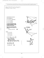
25. Motion of Connected Bodies

503–527


25.1. Introduction. 25.2. Motion of Two Bodies Connected by a String
and Passing over a Smooth Pulley. 25.3. Motion of Two Bodies Connected
by a String One of which is Hanging Free and the Other Lying on a
Smooth Horizontal Plane. 25.4. Motion of Two Bodies Connected by a
String One of which is Hanging Free and the Other Lying on a Rough
Horizontal Plane. 25.5. Motion of Two Bodies Connected by a String
One of which is Hanging Free and the Other Lying on a Smooth Inclined
Plane. 25.6. Motion of Two Bodies connected by a String, One of which
is Hanging Free and the Other is Lying on a Rough Inclined Plane.
25.7. Motion of Two Bodies Connected by a String and Lying on Smooth
Inclined Planes. 25.8. Motion of Two Bodies Connected by a String Lying
on Rough Inclined Planes.

(x)


26. Helical Springs and Pendulums

528–552

26.1. Introduction. 26.2. Helical Springs. 26.3. Helical Springs in Series
and Parallel. 26.4. Simple Pendulum. 26.5. Laws of Simple Pendulum.
26.6. Gain or Loss in the No. of Oscillations due to Change in the Length
of String or Acceleration due to Gravity of a Simple Pendulum.
26.7. Gain or Loss in the No. of Oscillations due to Change in the Position
of a Simple Pendulum. 26.8. Compound Pendulum. 26.9. Centre of
Oscillation (or Centre of Percussion). 26.10. Conical Pendulum.

27. Collision of Elastic Bodies


553–571

27.1. Introduction. 27.2. Phenomenon of Collision. 27.3. Law of
Conservation of Momentum. 27.4. Newton’s law of Collision of Elastic
Bodies. 27.5. Coefficient of Restitution. 27.6. Types of Collisions.
27.7. Direct Collision of Two Bodies. 27.8. Loss of Kinetic Energy During
Collision. 27.9. Indirect Impact of Two Bodies. 27.10. Direct Impact of a Body
with a Fixed Plane. 27.11. Indirect Impact of a Body with a Fixed Plane.

28. Motion Along a Circular Path

572–585

28.1. Introduction. 28.2. Centripetal Acceleration. 28.3. Centripetal Force.
28.4. Centrifugal Force. 28.5. Centrifugal Force Acting on a Body
Moving Along a Circular Path. 28.6. Superelevation. 28.7. Effect of
Superelevation in Roadways. 28.8. Effect of Superelevation in Railways.
28.9. Equilibrium Speed for Superelevation. 28.10. Reactions of a
Vehicle Moving along a Level Circular Path. 28.11. Equilibrium of a
Vehicle Moving along a Level Circular Path. 28.12. Maximum velocity to
Avoid Overturning of a Vehicle Moving along a Level Circular Path.
28.13. Maximum Velocity to Avoid Skidding Away of a Vehicle Moving
along a Level Circular Path.

29. Balancing of Rotating Masses

586–598

29.1. Introduction. 29.2. Methods for Balancing of Rotating Masses.
29.3. Types of Balancing of Rotating Masses. 29.4. Balancing of a Single

Rotating Mass. 29.5. Balancing of a Single Rotating Mass by Another
Mass in the Same Plane. 29.6. Balancing of a Single Rotating Mass by
Two Masses in Different Planes. 29.7. Balancing of Several Rotating
Masses. 29.8. Analytical Method for the Balancing of Several Rotating
Masses in one Plane by Another Mass in the Same Plane. 29.9. Graphical
Method for the Balancing of Several Rotating Masses in One Plane by
Another Mass in the Same Plane. 29.10. Centrifugal governor.
29.11. Watt Governor.

30. Work, Power and Energy

599–621

30.1. Introduction. 30.2. Units of Work. 30.3. Graphical Representation of
Work. 30.4. Power. 30.5. Units of Power. 30.6. Types of Engine Powers.
30.7. Indicated Power. 30.8. Brake Power. 30.9. Efficiency of an Engine.
30.10. Measurement of Brake Power. 30.11. Rope Brake Dynamometer.
30.12. Proney Brake Dynamometer. 30.13. Froude and Thornycraft
Transmission Dynamometer. 30.14. Motion on Inclined Plane.
30.15. Energy. 30.16. Units of Energy. 30.17. Mechanical Energy.
30.18. Potential Energy. 30.19. Kinetic Energy. 30.20. Transformation of
Energy. 30.21. Law of Conservation of Energy. 30.22. Pile and Pile Hammer.

31. Kinetics of Motion of Rotation

622–650

31.1. Introduction. 31.2. Torque. 31.3. Work done by a Torque.
31.4. Angular Momentum. 31.5. Newton’s Laws of Motion of Rotation.
31.6. Mass Moment of Inertia. 31.7. Mass Moment of Inertia of a Uniform

Thin Rod about the Middle Axis Perpendicular to the Length.
31.8. Moment of Inertia of a Uniform Thin Rod about One of the Ends
Perpendicular to the Length. 31.9. Moment of Inertia of a Thin Circular
Ring. 31.10. Moment of Inertia of a Circular Lamina. 31.11. Mass Moment
of Inertia of a Solid Sphere. 31.12. Units of Mass Moment of Inertia.
31.13. Radius of Gyration. 31.14. Kinetic Energy of Rotation.

(xi)


31.15. Torque and Angular Acceleration. 31.16. Relation Between Kinetics
of Linear Motion and Kinetics of Motion of Rotation. 31.17. Flywheel.
31.18. Motion of a Body Tied to a String and Passing Over a Pulley.
31.19. Motion of Two Bodies Connected by a String and Passing Over a
Pulley. 31.20. Motion of a Body Rolling on a Rough Horizontal Plane
without Slipping. 31.21. Motion of a Body Rolling Down a Rough Inclined
Plane without Slipping.

32. Motion of Vehicles

651–669

32.1. Introduction. 32.2. Types of Motions of Vehicles. 32.3. Motion of a
Vehicle Along a Level Track when the Tractive Force Passes Through its
Centre of Gravity. 32.4. Motion of a Vehicle Along a Level Track when
the Tractive Force Passes Through a Point Other than its Centre of Gravity.
32.5. Driving of a Vehicle. 32.6. Braking of a Vehicle. 32.7. Motion of
Vehicles on an Inclined Plane.

33. Transmission of Power by Belts and Ropes 670–695

33.1. Introduction. 33.2. Types of Belts. 33.3. Velocity Ratio of a Belt
Drive. 33.4. Velocity Ratio of a Simple Belt Drive. 33.5. Velocity Ratio
of a Compound Belt Drive. 33.6. Slip of the Belt. 33.7. Types of Belt
Drives. 33.8. Open Belt Drive. 33.9. Cross Belt Drive. 33.10. Length of
the Belt. 33.11. Length of an Open Belt Drive. 33.12. Length of a CrossBelt Drive. 33.13. Power Transmitted by a Belt. 33.14. Ratio of Tensions.
33.15. Centrifugal Tension. 33.16. Maximum Tension in the Belt.
33.17. Condition for Transmission of Maximum Power. 33.18. Belt Speed
for Maximum Power. 33.19. Initial Tension in the Belt. 33.20. Rope
Drive. 33.21. Advantages of Rope Drive. 33.22. Ratio of Tensions in
Rope Drive.

34. Transmission of Power by Gear Trains

696–717

34.1. Introduction. 34.2. Friction Wheels. 34.3. Advantages and
Disadvantages of a Gear Drive. 34.4. Important Terms. 34.5. Types of
Gears. 34.6. Simple Gear Drive. 34.7. Velocity Ratio of a Simple Gear
Drive. 34.8. Power Transmitted by a Simple Gear. 34.9. Train of Wheels.
34.10. Simple Trains of Wheels. 34.11. Compound Train of Wheels.
34.12. Design of Spur Wheels. 34.13. Train of Wheels for the Hour and
Minute Hands of a 12-Hour clock. 34.14. Epicyclic Gear Train.
34.15. Velocity Ratio of an Epicyclic Gear Train. 34.16. Compound
Epicyclic Gear Train (Sun and Planet Wheel). 34.17. Epicyclic Gear Train
with Bevel Wheels.

35. Hydrostatics

718–741


35.1. Introduction. 35.2. Intensity of Pressure. 35.3. Pascal’s Law.
35.4. Pressure Head. 35.5. Total Pressure. 35.6. Total Pressure on an
Immersed Surface. 35.7. Total Pressure on a Horizontally Immersed
Surface. 35.8. Total Pressure on a Vertically Immersed Surface. 35.9. Total
Pressure on an Inclined Immersed Surface. 35.10. Centre of Pressure.
35.11. Centre of Pressure of a Vertically lmmersed Surface. 35.12. Centre
of Pressure of an Inclined Immersed Surface. 35.13. Pressure Diagrams.
35.14. Pressure Diagram Due to One Kind of Liquid on One Side.
35.15. Pressure Diagram Due to One Kind of Liquid Over Another on
One Side. 35.16. Pressure Diagram Due to Liquids on Both Sides.
35.17. Centre of Pressure of a Composite Section.

36. Equilibrium of Floating Bodies

742–758

36.1. Introduction. 36.2. Archimedes’ Principle. 36.3. Buoyancy.
36.4. Centre of Buoyancy. 36.5. Metacentre. 36.6. Metacentric Height.
36.7. Analytical Method for Metacentric Height. 36.8. Types of Equilibrium
of a Floating Body. 36.9. Stable Equilibrium. 36.10. Unstable Equilibrium.
36.11. Neutral Equilibrium. 36.12. Maximum Length of a Body Floating
Vertically in Water. 36.13. Conical Buoys Floating in a Liquid.

Index

(xii)

759–765

Top



Contents

C H A P T E R

1

Introduction

Contents
1.

Science.

2.

Applied Science.

3.

Engineering Mehanics.

4.

Beginning and Development
of Engineering Mechanics.

5.


Divisions of Engineering
Mechanics.

6.

Statics.

7.

Dynamics.

8.

Kinetics.

9.

Kinematics.

10. Fundamental Units.
11. Derived Units.
12. Systems of Units.
13. S.I. Units (International
System of Units.).
14. Metre.
15. Kilogram.
16. Second.

1.1. SCIENCE


17. Presentation of Units and
Their Values.

In this modern age, the word ‘science’ has got
different meanings for different people. An ordinary
man takes it as ‘something’ beyond his understanding,
whereas others may take it as ‘mysteries of research’
which are understood only by a few persons
working amidst complicated apparatus in a laboratory.
A non-scientist feels that it is a ‘subject’ whose
endeavour is aimed to improve the man’s life on the
earth. A business executive has the idea that it is
‘something’ which solves our day to day manufacturing
and quality control problems, so that the nation’s
economic prosperity keeps on improving.

18. Rules for S.I. Units.
19. Useful Data.
20. Algebra.
21. Trigonometry.
22. Differential Calculus.
23. Integral Calculus.
24. Scalar Quantities.
25. Vector Quantities.

In fact, ‘science’ may be defined as the growth
of ideas through observation and experimentation. In
1



Contents

2 „ A Textbook of Engineering Mechanics
this sense, the subject of science does not, necessarily, has to contribute something to the welfare of
the human life, although the man has received many benefits from the scientific investigations.

1.2. APPLIED SCIENCE
Strictly speaking, the world of science is so vast that the present day scientists and
technologists have to group the various spheres of scientific activities according to some common
characteristics to facilitate their training and research programmes. All these branches of science,
still have the common principle of employing observation and experimentation. The branch of
science, which co-ordinates the research work, for practical utility and services of the mankind, is
known as Applied Science.

1.3. ENGINEERING MECHANICS
The subject of Engineering Mechanics is that branch of Applied Science, which deals with the
laws and principles of Mechanics, alongwith their applications to engineering problems. As a matter
of fact, knowledge of Engineering Mechanics is very essential for an engineer in planning, designing
and construction of his various types of structures and machines. In order to take up his job more
skilfully, an engineer must persue the study of Engineering Mechanics in a most systematic and
scientific manner.

1.4. BEGINNING AND DEVELOPMENT OF ENGINEERING MECHANICS
It will be interesting to know, as to how the early man had been curious to know about the
different processes going on the earth. In fact, he used to content himself, by holding gods responsible
for all the processes. For a long time, the man had been trying to improve his ways of working. The
first step, in this direction, was the discovery of a circular wheel, which led to the use of animal driven
carts. The study of ancient civilization of Babylonians, Egyptians, Greeks and Roman reveal the use
of water wheels and wind mills even during the pre-historic days.
It is believed that the word ‘Mechanics’ was coined by a Greek philosopher Aristotle

(384–322 BC). He used this word for the problems of lever and the concept of centre of gravity. At
that time, it included a few ideas, which were odd, unsystematic and based mostly on observations
containing incomplete information. The first mathematical concept of this subject was developed by
Archimedes (287–212 BC). The story, for the discovery of First Law of Hydrostatics, is very popular
even today in the history of the development of Engineering Mechanics. In the normal course, Hieron
king of Syracuse got a golden crown made for his use. He suspected that the crown has been made
with an adultrated gold. The king liked the design of the crown so much that he did not want it to be
melted,in order to check its purity. It
is said that the king announced a huge
reward for a person, who can check
the purity of the crown gold without
melting it. The legend goes that
Archimedes, a pure mathematician,
one day sitting in his bath room tub
realised that if a body is immersed in
water, its apparent weight is reduced.
He thought that the apparent loss of
weight of the immersed body is equal
to the weight of the liquid displaced.
Sir Issac Newton (1643–1727)
It is believed that without further


Contents

Chapter 1 : Introduction „ 3
thought, Archimedes jumeped out of the bath tub and ran naked down the street shouting ‘Eureka,
eureka !’ i.e. I have found it, I have found it !’
The subject did not receive any concrete contribution for nearly 1600 years. In 1325, Jean
Buridan of Paris University proposed an idea that a body in motion possessed a certain impetus

i.e. motion. In the period 1325–1350, a group of scientists led by the Thomas Bradwardene of
Oxford University did lot of work on plane motion of bodies. Leonarodo Da Vinci (1452–1519),
a great engineer and painter, gave many ideas in the study of mechanism, friction and motion of
bodies on inclined planes. Galileo (1564–1642) established the theory of projectiles and gave a
rudimentary idea of inertia. Huyghens (1629–1695) developed the analysis of motion of a
pendulum.
As a matter of fact, scientific history of Engineering Mechanics starts with Sir Issac Newton
(1643–1727). He introduced the concept of force and mass, and gave Laws of Motion in 1686.
James Watt introduced the term horse power for comparing performance of his engines. John Bernoulli
(1667–1748) enunciated the priciple of virtual work. In eighteenth century, the subject of Mechanics
was termed as Newtonian Mechanics. A further development of the subject led to a controversy
between those scientists who felt that the proper measure of force should be change in kinetic energy
produced by it and those who preferred the change in momentum. In the nineteenth century, many
scientists worked tirelessly and gave a no. of priciples, which enriched the scientific history of the
subject.
In the early twentieth century, a new technique of research was pumped in all activities of
science. It was based on the fact that progress in one branch of science, enriched most of the bordering
branches of the same science or other sciences. Similarly with the passage of time, the concept of
Engineering Mechanics aided by Mathematics and other physical sciences, started contributing
and development of this subject gained new momentum in the second half of this century. Today,
knowledge of Engineering Mechanics, coupled with the knowledge of other specialised subjects e.g.
Calculus, Vector Algebra, Strength of Materials, Theory of Machines etc. has touched its present
height. The knowledge of this subject is very essential for an engineer to enable him in designing his
all types of structures and machines.

1.5. DIVISIONS OF ENGINEERING MECHANICS
The subject of Engineering Mechanics may be divided into the following two main groups:
1. Statics, and 2. Dynamics.

1.6. STATICS

It is that branch of Engineering Mechanics, which deals with the forces and their effects, while
acting upon the bodies at rest.

1.7. DYNAMICS
It is that branch of Engineering Mechanics, which deals with the forces and their effects, while
acting upon the bodies in motion. The subject of Dynamics may be further sub-divided into the
following two branches :
1. Kinetics, and 2. Kinematics.

1.8. KINETICS
It is the branch of Dynamics, which deals with the bodies in motion due to the application
of forces.


Contents

4 „ A Textbook of Engineering Mechanics
1.9. KINEMATICS
It is that branch of Dynamics, which deals with the bodies in motion, without any reference
to the forces which are responsible for the motion.

1.10. FUNDAMENTAL UNITS
The measurement of physical quantities is one of the most important operations in engineering.
Every quantity is measured in terms of some arbitrary, but internationally accepted units, called
fundamental units.
All the physical quantities, met with in Engineering Mechanics, are expressed in terms of three
fundamental quantities, i.e.
1. length, 2. mass and 3. time.

1.11. DERIVED UNITS

Sometimes, the units are also expressed in other units (which are derived from fundamental
units) known as derived units e.g. units of area, velocity, acceleration, pressure etc.

1.12. SYSTEMS OF UNITS
There are only four systems of units, which are commonly used and universally recognised.
These are known as :
1. C.G.S. units, 2. F.P.S. units, 3. M.K.S. units and 4. S.I. units.
In this book, we shall use only the S.I. system of units, as the future courses of studies are
conduced in this system of units only.

1.13. S.I. UNITS (INTERNATIONAL SYSTEM OF UNITS)
The eleventh General Conference* of Weights and Measures has recommended a unified
and systematically constituted system of fundamental and derived units for international use. This
system of units is now being used in many countries.
In India, the Standards of Weights and Measures Act of 1956 (vide which we switched over to
M.K.S. units) has been revised to recognise all the S.I. units in industry and commerce.
In this system of units, the †fundamental units are metre (m), kilogram (kg) and second (s)
respectively. But there is a slight variation in their derived units. The following derived units will be
used in this book :
Density (Mass density)

kg / m3

Force

N (Newton)

Pressure

N/mm2 or N/m2


Work done (in joules)

J = N-m

Power in watts
W = J/s
International metre, kilogram and second are discussed here.
* It is knwon as General Conference of Weights and Measures (G.C.W.M.). It is an international organisation
of which most of the advanced and developing countries (including India) are members. This conference has been ensured the task of prescribing definitions of various units of weights and measures,
which are the very basis of science and technology today.
†

The other fundamental units are electric current, ampere (A), thermodynamic temperature, kelvin (K)
and luminous intensity, candela (cd). These three units will not be used in this book.


Contents

Chapter 1 : Introduction „ 5
1.14. METRE
The international metre may be defined as the shortest distance (at 0°C) between two parallel
lines engraved upon the polished surface of the Platinum-Iridium bar, kept at the International
Bureau of Weights and Measures at Sevres near Paris.

A bar of platinum - iridium metre kept at a
temperature of 0º C.

1.15. KILOGRAM
The international kilogram may be defined as the

mass of the Platinum-Iridium cylinder, which is also kept
at the International Bureau of Weights and Measures at
Sevres near Paris.

The standard platinum - kilogram is kept
at the International Bureau of Weights
and Measures at Serves in France.

1.16. SECOND
The fundamental unit of time for all the four systems is second, which is 1/(24 × 60 × 60) =
1/86 400th of the mean solar day. A solar day may be defined as the interval of time between the
instants at which the sun crosses the meridian on two consecutive days. This value varies throughout
the year. The average of all the solar days, of one year, is called the mean solar day.

1.17. PRESENTATION OF UNITS AND THEIR VALUES
The frequent changes in the present day life are facililtated by an international body
known as International Standard Organisation (ISO). The main function of this body is to
make recommendations regarding international procedures. The implementation of ISO
recommendations in a country is assisted by an organisation appointed for the purpose. In India,
Bureau of Indian Standard formerly known as Indian Standards Institution (ISI) has been
created for this purpose.
We have already discussed in the previous articles the units of length, mass and time. It is
always necessary to express all lengths in metres, all masses in kilograms and all time in seconds.
According to convenience, we also use larger multiples or smaller fractions of these units. As a
typical example, although metre is the unit of length; yet a smaller length equal to one-thousandth of
a metre proves to be more convenient unit especially in the dimensioning of drawings. Such convenient
units are formed by using a prefix in front of the basic units to indicate the multiplier.


Contents


6 „ A Textbook of Engineering Mechanics
The full list of these prefixes is given in Table 1.1.

Table 1.1
Factor by which the unit
is multiplied
1000 000 000 000
1 000 000 000
1 000 000
1 000
100
10
0.1
0.01
0.001
0.000 001
0.000 000 001
0.000 000 000 001

Standard form
1012
109
106
103
102
101
10–1
10–2
10–3

10–6
10–9
10–12

Prefix
Tera
giga
mega
kilo
hecto*
deca*
deci*
centi*
milli
micro
nano
pico

Abbreviation
T
G
M
k
h
da
d
c
m
μ
n

p

Note : These prefixes are generally becoming obsolete probably due to possible confusion.
Moreover, it is becoming a conventional practice to use only those powers of ten, which conform
to 03n (where n is a positive or negative whole number).

1.18. RULES FOR S.I. UNITS
The Eleventh General Conference of Weights and Measures recommended only the fundamental
and derived units of S.I. system. But it did not elaborate the rules for the usage of these units. Later
on, many scientists and engineers held a no. of meetings for the style and usage of S.I. units. Some of
the decisions of these meetings are :
1. A dash is to be used to separate units, which are multiplied together. For example, a
newton-meter is written as N-m. It should no be confused with mN, which stands for
millinewton.
2. For numbers having 5 or more digits, the digits should be placed in groups of three separated
by spaces (instead of *commas) counting both to the left and right of the decimal point.
3. In a †four digit number, the space is not required unless the four digit number is used in
a column of numbers with 5 or more digits.
At the time of revising this book, the author sought the advice of various international authorities
regarding the use of units and their values, keeping in view the global reputation of the author as well
as his books. It was then decided to ††present the units and their values as per the recommendations
of ISO and ISI. It was decided to use :
4500
not
4 500
or
4,500
7 589 000
not
7589000

or
7,589,000
0.012 55
not
0.01255
or
.01255
6
30 × 10
not
3,00,00,000
or
3 × 107
* In certain countries, comma is still used as the decimal marker.
† In certain countries, space is used even in a four digit number.
†† In some question papers, standard values are not used. The author has tried to avoid such questions in
the text of the book, in order to avoid possible confusion. But at certain places, such questions have been
included keeping in view the importance of question from the reader’s angle.


Contents

Chapter 1 : Introduction „ 7
The above mentioned figures are meant for numerical values only. Now we shall discuss about
the units. We know that the fundamental units in S.I. system for length, mass and time are metre,
kilogram and second respectively. While expressing these quantities, we find it time-consuming to
write these units such as metres, kilograms and seconds, in full, every time we use them. As a result of
this, we find it quite convenient to use the following standard abberviations, which are internationally
recognised. We shall use :
m

km
kg
t
s
min
N
N-m
kN-m
rad
rev

for metre or metres
for kilometre or kilometres
for kilogram or kilograms
for tonne or tonnes
for second or seconds
for minute or minutes
for newton or newtons
for newton × metres (i.e., work done)
for kilonewton × metres
for radian or radians
for revolution or revolutions

1.19. USEFUL DATA
The following data summarises the previous memory and formulae, the knowledge of which is
very essential at this stage.

1.20. ALGEBRA
1. a0 = 1 ; x0 = 1
(i.e., Anything raised to the power zero is one.)

2. xm × xn = xm + n
(i.e., If the bases are same, in multiplication, the powers are added.)
xm

= xm – n
xn
(i.e., If the bases are same in division, the powers are subtracted.)
4. If ax2 + bx + c = 0

3.

–b ± b 2 – 4ac
2a
where a is the coefficient of x2, b is the coefficient of x and c is the constant term.

then x =

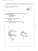
1.21. TRIGONOMETRY
In a right-angled triangle ABC as shown in Fig. 1.1
b
= sin θ
1.
c
a
= cos θ
2.
c
b sin θ
=
= tan θ

3.
a cos θ
Fig. 1.1.


Contents

8 „ A Textbook of Engineering Mechanics
c
1
=
= cosec θ
b sin θ
c
1
=
= sec θ
5.
a cos θ
a cos θ
1
=
=
= cot θ
6.
b sin θ tan θ
7. The following table shows values of trigonometrical functions for some typical angles:

4.


angle

0°

30°

45°

60°

90°

sin

0

1
2

1

3
2

1

cos

1


3
2

1
2

0

tan

0

2
1
2

1

1

3

∞

3

or in other words, for sin write
0°

30°


45°

60°

90°

0
2

1
2

3
2

4
2

0

1
2

2
2
1

3
2


1

2

for cos write the values in reverse order ; for tan divide the value of sin by cos for the
respective angle.
8. In the first quadrant (i.e., 0° to 90°) all the trigonometrical ratios are positive.
9. In the second quadrant (i.e., 90° to 180°) only sin θ and cosec θ are positive.
10. In the third quadrant (i.e., 180° to 270°) only tan θ and cot θ are positive.
11. In the fourth quadrant (i.e., 270° to 360°) only cos θ and sec θ are positive.
12. In any triangle ABC,
a
b
c
=
=
sin A sin B sin C
where a, b and c are the lengths of the three sides of a triangle. A, B and C are opposite
angles of the sides a, b and c respectively.
13. sin (A + B) = sin A cos B + cos A sin B
14. sin (A – B) = sin A cos B – cos A sin B
15. cos (A + B) = cos A cos B – sin A sin B
16. cos (A – B) = cos A cos B + sin A sin B
tan A + tan B
17. tan ( A + B) = 1 – tan A .tan B
tan A – tan B
18. tan ( A – B) = 1 + tan A .tan B
19. sin 2A = 2 sin A cos A



Contents

Chapter 1 : Introduction „ 9
20. sin2 θ + cos2 θ = 1
21. 1 + tan2 θ = sec2 θ
22. 1 + cot2 θ = cosec2 θ
1– cos 2 A
2
1
cos
2A
+
2
24. cos A =
2
25. 2 cos A sin B = sin (A + B) – sin ( A – B)
2
23. sin A =

26. Rules for the change of trigonometrical ratios:

( A)

( B)

(C )

⎧sin (– θ)
⎪cos (– θ)

⎪
⎪⎪ tan (– θ)
⎨
⎪cot (– θ)
⎪sec (– θ)
⎪
⎪⎩cosec (– θ)

= – sin θ
= cos θ

⎧sin (90° – θ)
⎪cos (90° – θ)
⎪
⎪⎪ tan (90° – θ)
⎨
⎪cot (90° – θ)
⎪sec (90° – θ)
⎪
⎪⎩cosec (90° – θ)

= cos θ
= sin θ

⎧sin (90° + θ)
⎪cos (90° + θ)
⎪
⎪⎪ tan (90° + θ)
⎨
⎪cot (90° + θ)

⎪sec (90° + θ)
⎪
⎪⎩cosec (90° + θ)

= cos θ
= – sin θ

= – tan θ
= – cot θ
= sec θ
= – cosec θ

= cot θ
= tan θ
= cosec θ
= sec θ

= – cot θ
= – tan θ
= – cosec θ
= sec θ

( D)

⎧sin (180° – θ) = sin θ
⎪cos (180° – θ) = – cos θ
⎪
⎪⎪ tan (180° – θ) = – tan θ
⎨
⎪cot (180° – θ) = – cot θ

⎪sec (180° – θ) = – sec θ
⎪
⎪⎩cosec (180° – θ) = cosec θ

(E)

⎧sin (180° + θ) = – sin θ
⎪cos (180° + θ) = – cos θ
⎪
⎪⎪ tan (180° + θ) = tan θ
⎨
⎪cot (180° + θ) = cot θ
⎪sec (180° + θ) = – sec θ
⎪
⎪⎩cosec (180° + θ) = – cosec θ


Contents

10 „ A Textbook of Engineering Mechanics
Following are the rules to remember the above 30 formulae :
Rule 1. Trigonometrical ratio changes only when the angle is (90° – θ)or (90° + θ). In all
other cases, trigonometrical ratio remains the same. Following is the law of change :
sin changes into cos and cos changes into sin,
tan changes into cot and cot changes into tan,
sec changes into cosec and cosec changes into sec.
Rule 2. Consider the angle θ to be a small angle and write the proper sign as per formulae
8 to 11 above.

1.22. DIFFERENTIAL CALCULUS

1.
2.

3.

4.

d
is the sign of differentiation.
dx

d
d
d
( x)n = nxn –1 ; ( x)8 = 8 x7 , ( x) = 1
dx
dx
dx
(i.e., to differentiate any power of x, write the power before x and subtract on from the
power).
d
d
(C ) = 0 ;
(7) = 0
dx
dx
(i.e., differential coefficient of a constant is zero).
d
dv
du

(u . v ) = u .
+ v.
dx
dx
dx

⎡i.e., Differential ⎤
⎢
coefficient of ⎥⎥
⎡(1st function × Differential coefficient of sec ond function) ⎤
⎢
= ⎢
⎥
⎢
product of any ⎥
⎣+ (2nd function × Differential coefficient of first function) ⎦
⎢
⎥
two functions ⎦⎥
⎣⎢

5.

d ⎛u⎞
⎜ ⎟=
dx ⎝ v ⎠

v.

du

dv
– u.
dx
dx
v2

⎡i.e., Differential coefficient of
⎢ two functions when one is
⎢
⎢⎣
divided by the other

⎤ ⎡( Denominator × Differential coefficient of numerator ) ⎤
⎥ =⎢
⎥
⎥ ⎢ – ( Numerator × Differential coefficient of denominator ) ⎥
⎥⎦ ⎢⎣
Square of denominator
⎥⎦

6. Differential coefficient of trigonometrical functions
d
d
(sin x) = cos x ;
(cos x ) = – sin x
dx
dx
d
d
(tan x) = sec 2 x ;

(cot x ) = – cosec2 x
dx
dx
d
d
(sec x) = sec x . tan x ;
(cosec x ) = – cosec x . cot x
dx
dx

(i.e., The differential coefficient, whose trigonometrical function begins with co, is negative).


Contents

Chapter 1 : Introduction „ 11
7. If the differential coefficient of a function is zero, the function is either maximum or minimum. Conversely, if the maximum or minimum value of a function is required, then differentiate the function and equate it to zero.

1.23. INTEGRAL CALCULUS
1.

∫ dx is the sign of integration.

2.

∫x

n

dx =


x n +1
x7
; ∫ x 6 dx =
7
n+1

(i.e., to integration any power of x, add one to the power and divide by the new power).
3.

∫ 7dx = 7 x ; ∫ C dx = Cx
(i.e., to integrate any constant, multiply the constant by x).

4.

n
∫ (ax + b) dx =

(ax + b)n +1
(n + 1) × a

(i.e., to integrate any bracket with power, add one to the power and divide by the new power
and also divide by the coefficient of x within the bracket).

1.24. SCALAR QUANTITIES
The scalar quantities (or sometimes known as scalars) are those quantities which have magnitude
only such as length, mass, time, distance, volume, density, temperature, speed etc.

1.25. VECTOR QUANTITIES
The vector quantities (or sometimes known as

vectors) are those quantities which have both magnitude
and direction such as force, displacement, velocity,
acceleration, momentum etc. Following are the important
features of vector quantities :
1. Representation of a vector. A vector is
represented by a directed line as shown in
Fig. 1.2. It may be noted that the length OA
—→
represents the magnitude of the vector OA
. The
—→
direction of the vector is OA
is from O (i.e.,

The velocity of this cyclist is an example
of a vector quantity.

starting point) to A (i.e., end point). It is also
2.
3.
4.
5.

known as vector P.
→
Unit vector. A vector, whose magnitude is unity,
Fig. 1.2. Vector OA
is known as unit vector.
Equal vectors. The vectors, which are parallel to each other and have same direction (i.e.,
same sense) and equal magnitude are known as equal vectors.

Like vectors. The vectors, which are parallel to each other and have same sense but unequal
magnitude, are known as like vectors.
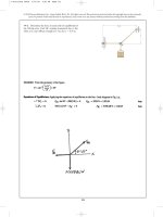
Addition of vectors. Consider two vectors PQ and RS, which are required to be added as
shown in Fig. 1.3. (a).


Contents

12 „ A Textbook of Engineering Mechanics

Fig. 1.3.

Take a point A, and draw line AB parallel and equal in magnitude to the vector PQ to some
convenient scale. Through B, draw BC parallel and equal to vector RS to the same scale. Join AC
which will give the required sum of vectors PQ and RS as shown in Fig. 1.3. (b).
This method of adding the two vectors is called the Triangle Law of Addition of Vectors.
Similarly, if more than two vectors are to be added, the same may be done first by adding the two
vectors, and then by adding the third vector to the resultant of the first two and so on. This method of
adding more than two vectors is called Polygon Law of Addition of Vectors.
6. Subtraction of vectors. Consider two vectors PQ and RS in which the vector RS is required
to be subtracted as shown in Fig. 1.4 (a)

Fig. 1.4.

Take a point A, and draw line AB parallel and equal in magnitude to the vector PQ to some
convenient scale. Through B, draw BC parallel and equal to the vector RS, but in opposite direction,
to that of the vector RS to the same scale. Join AC, which will give the resultant when the vector PQ
is subtracted from vector RS as shown in Fig. 1.4 (b).

Top



Contents

Chapter 2 : Composition and Resolution of Forces „ 13
C H A P T E R

2

Composition and
Resolution
of Forces

Contents
1.

Introduction.

2.

Effects of a Force.

3.

Characteristics of a Force.

4.

Principle of Physical
Independence of Forces.


5.

Principle of Transmissibility
of Forces.

6.

System of Forces.

7.

Resultant Force.

8.

Composition of Forces.

9.

Methods for the Resultant
Force.

10. Analytical Method for
Resultant Force.
11. Parallelogram Law of
Forces.
12. Resolution of a Force.
13. Principle of Resolution.
14. Method of Resolution for

the Resultant Force.
15. Laws for the Resultant
Force.
16. Triangle Law of Forces.
17. Polygon Law of Forces.
18. Graphical (vector) Method
for the Resultant Force.

2.1. INTRODUCTION
The force is an important factor in the field of
Mechanics, which may be broadly *defined as an agent
which produces or tends to produce, destroys or tends
to destroy motion. e.g., a horse applies force to pull a
cart and to set it in motion. Force is also required to
work on a bicycle pump. In this case, the force is
supplied by the muscular power of our arms and
shoulders.
*

It may be noted that the force may have either of the
two functions i.e., produces or tends to produce motion.
The second part of the definition is an application of
the first part. In statics, we consider the second function
of the force only i.e., ‘tends to produce motion.’
13