CHAPTER 32 THE INFLUENCE OF MONETARY AND FISCAL POLICY ON AGGREGATE DEMAND 745
right. There are two macroeconomic effects that make the size of the shift in ag-
gregate demand differ from the change in government purchases. The first—the
multiplier effect—suggests that the shift in aggregate demand could be larger than
$20 billion. The second—the crowding-out effect—suggests that the shift in aggre-
gate demand could be smaller than $20 billion. We now discuss each of these effects
in turn.
THE MULTIPLIER EFFECT
When the government buys $20 billion of goods from Boeing, that purchase has
repercussions. The immediate impact of the higher demand from the government
is to raise employment and profits at Boeing. Then, as the workers see higher earn-
ings and the firm owners see higher profits, they respond to this increase in in-
come by raising their own spending on consumer goods. As a result, the
government purchase from Boeing raises the demand for the products of many
other firms in the economy. Because each dollar spent by the government can raise
the aggregate demand for goods and services by more than a dollar, government
purchases are said to have a multiplier effect on aggregate demand.
This multiplier effect continues even after this first round. When consumer
spending rises, the firms that produce these consumer goods hire more people and
experience higher profits. Higher earnings and profits stimulate consumer spend-
ing once again, and so on. Thus, there is positive feedback as higher demand leads
to higher income, which in turn leads to even higher demand. Once all these ef-
fects are added together, the total impact on the quantity of goods and services
demanded can be much larger than the initial impulse from higher government
spending.
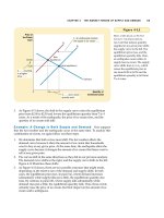
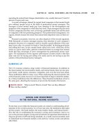
Figure 32-4 illustrates the multiplier effect. The increase in government pur-
chases of $20 billion initially shifts the aggregate-demand curve to the right from
AD
1
to AD
2

by exactly $20 billion. But when consumers respond by increasing
their spending, the aggregate-demand curve shifts still further to AD
3
.
This multiplier effect arising from the response of consumer spending can be
strengthened by the response of investment to higher levels of demand. For in-
stance, Boeing might respond to the higher demand for planes by deciding to buy
more equipment or build another plant. In this case, higher government demand
spurs higher demand for investment goods. This positive feedback from demand
to investment is sometimes called the investment accelerator.
A FORMULA FOR THE SPENDING MULTIPLIER
A little high school algebra permits us to derive a formula for the size of the mul-
tiplier effect that arises from consumer spending. An important number in this for-
mula is the marginal propensity to consume (MPC)—the fraction of extra income that
a household consumes rather than saves. For example, suppose that the marginal
propensity to consume is 3/4. This means that for every extra dollar that a house-
hold earns, the household spends $0.75 (3/4 of the dollar) and saves $0.25. With an
MPC of 3/4, when the workers and owners of Boeing earn $20 billion from the
government contract, they increase their consumer spending by 3/4 ϫ $20 billion,
or $15 billion.
multiplier effect
the additional shifts in aggregate
demand that result when
expansionary fiscal policy
increases income and thereby
increases consumer spending
746 PART TWELVE SHORT-RUN ECONOMIC FLUCTUATIONS
To gauge the impact on aggregate demand of a change in government pur-
chases, we follow the effects step-by-step. The process begins when the govern-
ment spends $20 billion, which implies that national income (earnings and profits)

also rises by this amount. This increase in income in turn raises consumer spend-
ing by MPC ϫ $20 billion, which in turn raises the income for the workers and
owners of the firms that produce the consumption goods. This second increase in
income again raises consumer spending, this time by MPC ϫ (MPC ϫ $20 billion).
These feedback effects go on and on.
To find the total impact on the demand for goods and services, we add up all
these effects:
Change in government purchases ϭ $20 billion
First change in consumption ϭ MPC ϫ $20 billion
Second change in consumption ϭ MPC
2
ϫ $20 billion
Third change in consumption ϭ MPC
3
ϫ $20 billion
••
••
••
Total change in demand ϭ
(1 ϩ MPC ϩ MPC
2
ϩ MPC
3
ϩ
· · ·
) ϫ $20 billion.
Here, “. . .” represents an infinite number of similar terms. Thus, we can write the
multiplier as follows:
Quantity of
Output

Price
Level
0
Aggregate demand,
AD
1
$20 billion
AD
2
AD
3
1. An increase in government purchases
of $20 billion initially increases aggregate
demand by $20 billion . . .
2. . . . but the multiplier
effect can amplify the
shift in aggregate
demand.
Figure 32-4
T
HE
M
ULTIPLIER
E
FFECT
.An
increase in government
purchases of $20 billion can
shift the aggregate-demand
curve to the right by more than

$20 billion. This multiplier
effect arises because increases
in aggregate income
stimulate additional
spending by consumers.
CHAPTER 32 THE INFLUENCE OF MONETARY AND FISCAL POLICY ON AGGREGATE DEMAND 747
Multiplier ϭ 1 ϩ MPC ϩ MPC
2
ϩ MPC
3
ϩ
· · · ·
This multiplier tells us the demand for goods and services that each dollar of gov-
ernment purchases generates.
To simplify this equation for the multiplier, recall from math class that this ex-
pression is an infinite geometric series. For x between Ϫ1 and ϩ1,
1 ϩ x ϩ x
2
ϩ x
3
ϩ
· · ·
ϭ 1/(1 Ϫ x).
In our case, x ϭ MPC. Thus,
Multiplier ϭ 1/(1 Ϫ MPC).
For example, if MPC is 3/4, the multiplier is 1/(1 Ϫ 3/4), which is 4. In this case,
the $20 billion of government spending generates $80 billion of demand for goods
and services.
This formula for the multiplier shows an important conclusion: The size of the
multiplier depends on the marginal propensity to consume. Whereas an MPC of

3/4 leads to a multiplier of 4, an MPC of 1/2 leads to a multiplier of only 2. Thus,
a larger MPC means a larger multiplier. To see why this is true, remember that the
multiplier arises because higher income induces greater spending on consump-
tion. The larger the MPC is, the greater is this induced effect on consumption, and
the larger is the multiplier.
OTHER APPLICATIONS OF THE MULTIPLIER EFFECT
Because of the multiplier effect, a dollar of government purchases can generate
more than a dollar of aggregate demand. The logic of the multiplier effect, how-
ever, is not restricted to changes in government purchases. Instead, it applies to
any event that alters spending on any component of GDP—consumption, invest-
ment, government purchases, or net exports.
For example, suppose that a recession overseas reduces the demand for U.S.
net exports by $10 billion. This reduced spending on U.S. goods and services de-
presses U.S. national income, which reduces spending by U.S. consumers. If the
marginal propensity to consume is 3/4 and the multiplier is 4, then the $10 billion
fall in net exports means a $40 billion contraction in aggregate demand.
As another example, suppose that a stock-market boom increases households’
wealth and stimulates their spending on goods and services by $20 billion. This ex-
tra consumer spending increases national income, which in turn generates even
more consumer spending. If the marginal propensity to consume is 3/4 and the
multiplier is 4, then the initial impulse of $20 billion in consumer spending trans-
lates into an $80 billion increase in aggregate demand.
The multiplier is an important concept in macroeconomics because it shows
how the economy can amplify the impact of changes in spending. A small initial
change in consumption, investment, government purchases, or net exports can
end up having a large effect on aggregate demand and, therefore, the economy’s
production of goods and services.
748 PART TWELVE SHORT-RUN ECONOMIC FLUCTUATIONS
THE CROWDING-OUT EFFECT
The multiplier effect seems to suggest that when the government buys $20 billion

of planes from Boeing, the resulting expansion in aggregate demand is necessarily
larger than $20 billion. Yet another effect is working in the opposite direction.
While an increase in government purchases stimulates the aggregate demand for
goods and services, it also causes the interest rate to rise, and a higher interest rate
reduces investment spending and chokes off aggregate demand. The reduction in
aggregate demand that results when a fiscal expansion raises the interest rate is
called the crowding-out effect.
To see why crowding out occurs, let’s consider what happens in the money
market when the government buys planes from Boeing. As we have discussed,
this increase in demand raises the incomes of the workers and owners of this firm
(and, because of the multiplier effect, of other firms as well). As incomes rise,
households plan to buy more goods and services and, as a result, choose to hold
more of their wealth in liquid form. That is, the increase in income caused by the
fiscal expansion raises the demand for money.
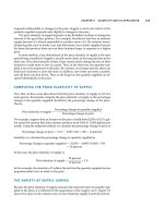
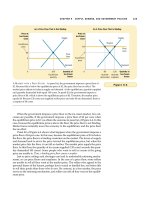
The effect of the increase in money demand is shown in panel (a) of Fig-
ure 32-5. Because the Fed has not changed the money supply, the vertical supply
curve remains the same. When the higher level of income shifts the money-
demand curve to the right from MD
1
to MD
2
, the interest rate must rise from r
1
to
r
2
to keep supply and demand in balance.
The increase in the interest rate, in turn, reduces the quantity of goods and ser-
vices demanded. In particular, because borrowing is more expensive, the demand
for residential and business investment goods declines. That is, as the increase in

government purchases increases the demand for goods and services, it may also
crowd out investment. This crowding-out effect partially offsets the impact of gov-
ernment purchases on aggregate demand, as illustrated in panel (b) of Figure 32-5.
The initial impact of the increase in government purchases is to shift the aggregate-
demand curve from AD
1
to AD
2
, but once crowding out takes place, the aggregate-
demand curve drops back to AD
3
.
To sum up: When the government increases its purchases by $20 billion, the aggre-
gate demand for goods and services could rise by more or less than $20 billion, depending
on whether the multiplier effect or the crowding-out effect is larger.
CHANGES IN TAXES
The other important instrument of fiscal policy, besides the level of government
purchases, is the level of taxation. When the government cuts personal income
taxes, for instance, it increases households’ take-home pay. Households will save
some of this additional income, but they will also spend some of it on consumer
goods. Because it increases consumer spending, the tax cut shifts the aggregate-
demand curve to the right. Similarly, a tax increase depresses consumer spending
and shifts the aggregate-demand curve to the left.
The size of the shift in aggregate demand resulting from a tax change is also af-
fected by the multiplier and crowding-out effects. When the government cuts taxes
and stimulates consumer spending, earnings and profits rise, which further stim-
ulates consumer spending. This is the multiplier effect. At the same time, higher
income leads to higher money demand, which tends to raise interest rates. Higher
crowding-out effect
the offset in aggregate demand that

results when expansionary fiscal
policy raises the interest rate and
thereby reduces investment spending
CHAPTER 32 THE INFLUENCE OF MONETARY AND FISCAL POLICY ON AGGREGATE DEMAND 749
interest rates make borrowing more costly, which reduces investment spending.
This is the crowding-out effect. Depending on the size of the multiplier and
crowding-out effects, the shift in aggregate demand could be larger or smaller than
the tax change that causes it.
In addition to the multiplier and crowding-out effects, there is another impor-
tant determinant of the size of the shift in aggregate demand that results from a tax
change: households’ perceptions about whether the tax change is permanent or
temporary. For example, suppose that the government announces a tax cut of
$1,000 per household. In deciding how much of this $1,000 to spend, households
must ask themselves how long this extra income will last. If households expect the
Quantity
of Money
Quantity fixed
by the Fed
0
Interest
Rate
r
2
r
1
Money demand,
MD
1
Money
supply

(a) The Money Market
3. . . . which
increases
the
equilibrium
interest
rate . . .
2. . . . the increase in
spending increases
money demand . . .
MD
2
Quantity
of Output
0
Price
Level
Aggregate demand,
AD
1
(b) The Shift in Aggregate Demand
4. . . . which in turn
partly offsets the
initial increase in
aggregate demand.
AD
2
AD
3
$20 billion

1. When an
increase in
government
purchases
increases
aggregate
demand . . .
Figure 32-5
T
HE
C
ROWDING
-O
UT
E
FFECT
.
Panel (a) shows the money
market. When the government
increases its purchases of goods
and services, the resulting
increase in income raises the
demand for money from MD
1
to MD
2
, and this causes the
equilibrium interest rate to rise
from r
1

to r
2
. Panel (b) shows the
effects on aggregate demand.
The initial impact of the increase
in government purchases shifts
the aggregate-demand curve
from AD
1
to AD
2
. Yet, because
the interest rate is the cost of
borrowing, the increase in the
interest rate tends to reduce
the quantity of goods and
services demanded, particularly
for investment goods. This
crowding out of investment
partially offsets the impact of
the fiscal expansion on
aggregate demand. In the end,
the aggregate-demand curve
shifts only to AD
3
.