nhiet dong hoc tap 1

Bạn đang xem bản rút gọn của tài liệu. Xem và tải ngay bản đầy đủ của tài liệu tại đây (14.89 MB, 634 trang )

(1)y op r C fo n d se tio se l U ua en a al ic ion Ev t L uct o N str In. MODERN PHYSICS FOR SCIENCE AND ENGINEERING First Edition Marshall L. Burns, Tuskegee University. Copyright © 2012 by Physics Curriculum & Instruction, Inc. www.PhysicsCurriculum.com ISBN: 978-0-9713134-4-6 Produced in the United States of America All Rights Reserved. This electronic textbook is protected by United States and International Copyright Law and may only be used in strict accordance with the purchased license agreement. Unauthorized duplication and/or distribution of this electronic textbook is a violation of copyright law and subject to severe criminal penalties..

(2) Electronic Textbook License Agreement. MODERN PHYSICS FOR SCIENCE AND ENGINEERING First Edition BY. MARSHALL L. BURNS. License Purchased: Single-Copy. y op r C fo n d se tio se l U ua en a al ic ion Ev t L uct o N str In. Physics Curriculum & Instruction hereby grants you a perpetual non-transferable license to use Modern Physics for Science and Engineering electronic textbook. In conjunction with a valid serial number, this license allows you to use the electronic textbook on a single computer only for personal use. The electronic textbook may not be placed on a network, whether or not it will be shared. Use on more than a single computer is a violation of this license. Any attempt to remove or alter the security features of this electronic textbook will result in this license being revoked and forfeiture of the right to use this electronic textbook. No portion of the electronic textbook may be copied or extracted, including: text, equations, illustrations, graphics, and photographs. The electronic textbook may only be used in its entirety. All components, including this license agreement, must remain locked together. Modern Physics for Science and Engineering is published and copyrighted by Physics Curriculum & Instruction and is protected by United States and International Copyright Law. Unauthorized duplication and/or distribution of copies of this electronic textbook is a violation of copyright law and subject to severe criminal penalties.. For further information or questions concerning this agreement, contact: Physics Curriculum & Instruction www.PhysicsCurriculum.com email: tel: 952-461-3470.

(3) i. C. O N T E N T S. Click on any topic below to be brought to that page. To return to this page, type “i” into the page number field.. Inside Cover iv. y op r C fo n d se tio se l U ua en a al ic ion Ev ot L uct N str In. Preface. Physical Constants, Common Derivatives . . .. 1 Classical Transformations 1 1.1 1.2 1.3 1.4 1.5 1.6. Introduction 1 Fundamental Units 3 Review of Classical Mechanics 4 Classical Space-Time Transformations 9 Classical Velocity and Acceleration Transformations 12 Classical Doppler Effect 16 Historical and Conceptual Perspective 24 Review of Fundamental and Derived Equations Problems 28. 4 Transformations of Relativistic Dynamics 96 4.1 4.2 4.3 4.4 4.5 4.6. 27. 2 Basic Concepts of Einsteinian Relativity 34 Introduction 34 2.1 Einstein’s Postulates of Special Relativity 36 2.2 Lengths Perpendicular to the Axis of Relative Motion 38 2.3 Time Interval Comparisons 41 2.4 Lengths Parallel to the Axis of Relative Motion 2.5 Simultaneity and Clock Synchronization 49 2.6 Time Dilation Paradox 52 Review of Derived Equations 55 Problems 56. 3 Transformations of Relativistic Kinematics 3.1 3.2 3.3 3.4 3.5 3.6. 62. Introduction 62 Relativistic Spatial Transformations 63 Relativistic Temporal Transformations 65 Comparison of Classical and Relativistic Transformations 67 Relativistic Velocity Transformations 72 Relativistic Acceleration Transformations 78 Relativistic Frequency Transformations 80 Review of Derived Equations 86 Problems 88. 44. Introduction 96 Relativistic Mass 97 Relativistic Force 104 Relativistic Kinetic and Total Energy 106 Relativistic Momentum 110 Energy and Inertial Mass Revisited 112 Relativistic Momentum and Energy Transformations 115 Review of Derived Equations 121 Problems 122. 5 Quantization of Matter 129. Introduction 129 5.1 Historical Perspective 130 5.2 Cathode Rays 132 5.3 Measurement of the Speciﬁc Charge e/me of Electrons 134 Speed of Electrons 136 Analysis of e/me Using the B-ﬁeld Deﬂection of Electrons 137 Analysis of e/me Using the CathodeAnode Potential 139 Analysis of e/me Using the E-ﬁeld Deﬂection of Electrons 140 5.4 Measurement of the Charge of an Electron 143 5.5 Determination of the Size of an Electron 148 5.6 Canal Rays and Thomson’s Mass Spectrograph 151 5.7 Modern Model of the Atom 156 5.8 Speciﬁc and Molal Atomic Masses 158 5.9 Size and Binding Energy of an Atom 163 Review of Fundamental and Derived Equations 167 Problems 170.

(4) ii. Contents. 6 Quantization of Electromagnetic Radiation 179. Introduction 333 9.1 One-Dimensional Time-Dependent Schrödinger Equation 334 9.2 Three-dimensional Time-Dependent Schrödinger Equation 338 9.3 Time-Independent Schrödinger Equation 340 9.4 Probability Interpretation of the Wave Function 343 9.5 Conservation of Probability 346 9.6 Free Particle and a Constant Potential 349 9.7 Free Particle in a Box (Inﬁnite Potential Well) 354 Conductions Electrons in One Dimension 361 Review of Fundamental and Derived Equations 363 Problems 366. y op r C fo n d se tio se l U ua en a al ic ion Ev ot L uct N str In. Introduction 179 6.1 Properties and Origin of Electromagnetic Waves 181 6.2 Intensity, Pressure, and Power of Electromagnetic Waves 188 6.3 Diffraction of Electromagnetic Waves 193 6.4 Energy and Momentum of Electromagnetic Radiation 196 6.5 Photoelectric Effect 201 6.6 Classical and Quantum Explanations of the Photoelectric Effect 204 6.7 Quantum Explanation of the Compton Effect 211 6.8 Relativistic Doppler Effect Revisited 216 Review of Fundamental and Derived Equations 219 Problems 223. 9 Schrödinger’s Quantum Mechanics 1 333. 10 Schrödinger’s Quantum Mechanics 11 376. 7 Quantization of One-Electron Atoms 232. Introduction 232 Atomic Spectra 235 Classical Model of the One-Electron Atom 237 Bohr Model of the One-Electron Atom 242 Emission Spectra and the Bohr Model 249 Correction to the Bohr Model for a Finite Nuclear Mass 253 7.6 Wilson-Sommerfeld Quantization Rule 260 Quantization of Angular Momentum for the Bohr Electron 260 Quantization of a Linear Harmonic Oscillator 262 7.7 Quantum Numbers and Electron Conﬁgurations 267 Review of Fundamental and Derived Equations 275 Problems 279 7.1 7.2 7.3 7.4 7.5. 8 Introduction to Quantum Mechanics 287. Introduction 287 Equation of Motion for a Vibrating String 288 Normal Modes ofVibration for the Stretched String 291 Traveling Waves and the Classical Wave Equation 295 De Broglie’s Hypothesis 299 Consistency with Bohr’s Quantization Hypothesis 301 Consistency with Einsteinian Relativity 305 8.5 Matter Waves 307 8.6 Group, Phase, and Particle Velocities 310 8.7 Heisenberg’s Uncertainty Principle 315 Review of Fundamental and Derived Equations 317 Problems 322. 8.1 8.2 8.3 8.4. Introduction 376 10.1 Wave Functions in Position and Momentum Representations 377 Dirac Delta Function 378 Free Particle Position and Momentum Wave Functions 381 10.2 Expectation Values 382 10.3 Momentum and Position Operators 387 Momentum Eigenvalues of a Free Particle in a One-Dimensional Box 394 10.4 Example: Expectation Values in Position and Momentum Space 396 Linear Harmonic Oscillator 401 10.5 Energy Operators 403 Hamiltonian Operator 406 10.6 Correspondence between Quantum and Classical Mechanics 407 Operator Algebra 411 10.7 Free Particle in a Three-Dimensional Box 414 Free Electron Gas in Three-Dimensions 418 Review of Fundamental and Derived Equations 423 Problems 428.

(5) Contents. 11 Classical Statistical Mechanics 439. 12 Quantum Statistical Mechanics 510 12.1 12.2. 12.3. 12.4 12.5. 12.6 12.7. Appendix A Basic Mathematics. A-1. A.1 Mathematical Symbols A-1 A.2 Exponential Operations A-1 A.3 Logarithmic Operations A-3 A.4 Scientiﬁc Notation and Useful Metric Preﬁxes A.5 Quadratic Equations A-5 A.6 Trigonometry A-6 A.7 Algebraic Series A-9 A.8 Basic Calculus A-10 A.9 Vector Calculus A-13 A.10 Deﬁnite Integrals A-16 Problems A-17. y op r C fo n d se tio se l U ua en a al ic ion Ev ot L uct N str In. Introduction 439 11.1 Phase Space and the Microcanonical Ensemble 441 11.2 System Conﬁgurations and Complexions: An Example 443 11.3 Thermodynamic Probability 447 Ensemble Averaging 451 Entropy and Thermodynamic Probability 453 11.4 Most Probable Distribution 457 11.5 Identiﬁcation of b 460 b and the Zeroth Law of Thermodynamics 461 Evaluation of b 462 11.6 Signiﬁcance of the Partition Function 466 11.7 Monatomic Ideal Gas 472 Energy, Entropy, and Pressure Formulae 472 Energy, Momentum, and Speed Distribution Formulae 479 11.8 Equipartition of Energy 485 Classical Speciﬁc Heat 488 Review of Fundamental and Derived Equations 491 Problems 495. Introduction 510 Formulation of Quantum Statistics 512 Thermodynamic Probabilities in Quantum Statistics 516 Maxwell-Boltzmann Statistics Revisited 517 Bose-Einstein Statistics 519 Fermi-Dirac Statistics 521 Most Probable Distribution 523 Bose-Einstein Distribution 524 Fermi-Dirac Distribution 526 Classical Limit of Quantum Distributions 527 Identiﬁcation of the Lagrange Multipliers 530 Speciﬁc Heat of a Solid 533 Einstein Theory (M-B Statistics) 534 Debye Theory (Phonon Statistics) 540 Blackbody Radiation (Photon Statistics) 545 Free Electron Theory of Metals (F-D Statistics) 551 Fermi Energy 552 Electronic Energy and Speciﬁc Heat Formulae 557 Review of Fundamental and Derived Equations 560 Problems 565. iii. Appendix B. Properties of Atoms in Bulk. A-21. Appendix C. Partial List of Nuclear Masses Index. 1-1. A-24. A-4.

(6) iv. P R E F A C E. y op r C fo n d se tio se l U ua en a al ic ion Ev ot L uct N str In. This book provides an introduction to modern physics for students who have completed an academic year of general physics. As a continuation of introductory general physics, it includes the subject areas of classical relativity (Chapter 1), Einstein’s special theory of relativity (Chapters 224), the old quantum theory (Chapters 527), an introduction to quantum mechanics (Chapters 8210), and introductory classical and quantum statistical mechanics (Chapters 11212). In a two-term course, Chapters 127 may be covered in the ﬁrst term and Chapters 8212 in the second. For schools offering a one-term course in modern physics, many of the topics in Chapters 127 may have previously been covered; consequently, the portions of this textbook to be covered might include parts of the old quantum theory, all of quantum mechanics, and possibly some of the topics in statistical mechanics. It is important to recognize that mathematics is only a tool in the development of physical theories and that the mathematical skills of students at the sophomore level are often limited. Accordingly, algebra and basic trigonometry are primarily used in Chapters 127, with elementary calculus being introduced either as an alternative approach or when necessary to preserve the integrity and rigor of the subject. The math review provided in Appendix A is more than sufﬁcient for a study of the entire book. On occasions when higher mathematics is required, as with the solution to a second-order partial differential equation in Chapter 8, the mathematics is sufﬁciently detailed to allow understanding with only a.

(7) v. Preface. y op r C fo n d se tio se l U ua en a al ic ion Ev ot L uct N str In. knowledge of elementary calculus. Even quantum theory and statistical mechanics are easily managed with this approach through the introduction of operator algebra and with the occasional use of one of the ﬁve deﬁnite integrals provided in Appendix A. This reduced mathematical emphasis allows students to concentrate on the more important underlying physical concepts and not be distracted or intimidated by unfamiliar mathematics. A major objective of this book is to enhance student understanding and appreciation of the fundamentals of physics by illustrating the necessary physical and quantitative reasoning with fundamentals that is essential for theoretical modeling of phenomena in science and engineering. The majority of physics textbooks at both the introductory and the intermediate level concentrate on introducing the basic concepts, formulas, and associated terminology of a broad spectrum of physics topics, leaving little space for the development of mathematical logic and physical reasoning from ﬁrst principles. Certainly, students must ﬁrst learn the fundamentals of the subject before intricate, detailed logic and reasoning are possible. But most intermediate and advanced books follow the lead of introductory textbooks and seldom elaborate in sufﬁcient detail the development of physical theories. Students are expected somehow to develop the necessary physical and quantitative reasoning either on their own or from classroom lectures. The result is that many students simply memorize physical formulas and stereotyped problems in their initial study of physics and continue the practice in intermediate and advanced courses. Students entering college are often accomplished at rote memorization but poorly prepared in reasoning skills. They must learn how to reason and how to employ logic with a set of fundamentals to obtain insights and results that are not obvious or commonly recognized. Developing understanding and reasoning is difﬁcult in the qualitative nonscience courses and supremely challenging in such highly quantitative courses as physics and engineering. The objective is, however, most desirable in these areas, since memorized equations and problems are rapidly forgotten by even the best students. In this textbook, a deliberate and detailed approach has been employed. All of the topics presented are developed from ﬁrst principles. In fact, all but three equations are rigorously derived via physical reasoning before being applied to problems or used in the discussion of other topics. Thus, the order of topics throughout the text is dictated by the requirement that fundamentals and physical derivations be carefully and judiciously introduced. And there is a gradual increase in the complexity of topics being considered to allow students to mature steadily in physical and quantitative reasoning as they progress through the book. For example, relativity is discussed early, since it depends on only a small number of physical fundamentals from kinematics and dynamics of general classical mechanics. Chapter 1 allows students to review pertinent fundamental.

(8) Preface. y op r C fo n d se tio se l U ua en a al ic ion Ev ot L uct N str In. equations of classical mechanics and to apply them to classical relativity before they are employed in the development of Einstein’s special theory of relativity in Chapters 224. This allows students time to develop the necessary quantitative skills and gain an overview of relativity before considering the conceptually subtle points of Einsteinian relativity. This basic approach, of reviewing the classical point of view before developing that of modern physics, continues throughout the text, to allow students to build upon what they already know an to develop strong connections between classical and modern physics. With this approach}where later subject areas are dependent on the fundamentals and results of earlier sections}students are led to develop greater insights as they apply previously gained knowledge to new physical situations. They also see how concepts of classical and modern physics are tied together, rather than seeing them as confused, isolated areas of interest. This development of reasoning skills and fundamental understanding better prepares students for all higher level courses. This book does not therefore pretend to be a survey of all modern physics topics. The pace of developing scientiﬁc understanding requires that some topics be omitted. For example, since a rigorous development of nuclear physics requires relativistic quantum mechanics, only a few basic topics (e.g., the size of the nucleus, nuclear binding energy, etc.) merit development within the pedagogic framework of the text. The goal of this book is to provide the background required for meaningful future studies and not to be a catalog of modern physics topics. Thus, the traditional coverage of nuclear physics has been displaced by the extremely useful subject of statistical mechanics. The fundamentals of statistical mechanics are carefully developed and applied to numerous topics in solid state physics and engineering, topics which themselves are so very important for many courses at the intermediate and advanced levels. The following pedagogic features appear throughout this textbook:. 1. Each chapter begins with an introductory overview of the direction and objectives of the chapter. 2. Boldface type is used to emphasize important concepts, principles, postulates, equation titles. and new terminology when they are ﬁrst introduced; thereafter, they may be italicized to reemphasize their importance. 3. Verbal deﬁnitions are set off by the use of italics. 4. Reference titles (and comments) for important equations appear in the margin of the text. 5. Fundamental deﬁning equations and important results from derivations are highlighted in color. Furthermore, a deﬁning symbol is used with fundamental deﬁning equations in place of an equality sign.. vi.

(9) vii. Preface. y op r C fo n d se tio se l U ua en a al ic ion Ev ot L uct N str In. 6. A logical and comprehensive list of the fundamental and derived equations in each chapter appears in a review section. It will assist students in the assimilation of fundamental equations (and associated reference terminology) and test their quantitative reasoning ability. 7. Formal solutions for the odd-numbered problems are provided at the end of each chapter, and answers are given for the even-numbered problems. A student’s efﬁciency in assimilating fundamentals and developing quantitative reasoning is greatly enhanced by making solutions an integral part of the text. The problems generally require students to be deliberate, reﬂective, and straightforward in their logic with physical fundamentals. 8. Examples and applications of physical theories are limited in order not to distract students from the primary aim of understanding the physical reasoning, fundamentals, and objectives of each section or chapter. Having solutions to problems at the end of a chapter reduces the number of examples required within the text, since many of the problems complement the chapter sections with subtle concepts being further investigated and discussed. 9. Endpapers provide a quick reference of frequently used quantities: the Greek alphabet, metric preﬁxes, mathematical symbols, calculus identities, and physical constants. Marshall L. Burns.

(10) 1. CH. A P T E R. 1. Classical Transformations. y op r C fo n d se tio se l U ua en a al ic ion Ev ot L uct N str In Classical mechanics and Galilean relativity apply to everyday objects traveling with relatively low speeds.. In experimental philosophy we are to look upon propositions obtained by general induction from phenomena as accurately or very nearly true . . . till such a time as other phenomena occur, by which they may either be made accurate, or liable to exception. SIR ISAAC NEWTON, Principia. (1686). Introduction Before the turn of the twentieth century, classical physics was fully developed within the three major disciplines—mechanics, thermodynamics, and electromagnetism. At that time the concepts, fundamental principles, and theories of classical physics were generally in accord with common sense.

(11) 2. Ch. 1 Classical Transformations. y op r C fo n d se tio se l U ua en a al ic ion Ev ot L uct N str In. and highly developed in precise, sophisticated mathematical formalisms. Alternative formulations to Newtonian mechanics were available through Lagrangian dynamics, Hamilton’s formulation, and the Hamilton-Jacobi theory, which were equivalent physical descriptions of nature but differed mathematically and philosophically. By 1864 the theory of electromagnetism was completely contained in a set of four partial differential equations. Known as Maxwell’s equations, they embodied all of the laws of electricity, magnetism, optics, and the propagation of electromagnetic radiation. The applicability and degree of sophistication of theoretical physics by the end of the nineteenth century was such that is was considered to be practically a closed subject. In fact, during the early 1890s some physicists purported that future accomplishments in physics would be limited to improving the accuracy of physical measurements. But, by the turn of the century, they realized classical physics was limited in its ability to accurately and completely describe many physical phenomena. For nearly 200 years after Newton’s contribution to classical mechanics, the disciplines of physics enjoyed an almost ﬂawless existence. But at the turn of the twentieth century there was considerable turmoil in theoretical physics, instigated in 1900 by Max Planck’s theory for the quantization of atoms regarded as electromagnetic oscillators and in 1905 by Albert Einstein’s publication of the special theory of relativity. The latter work appeared in a paper entitled “On the Electrodynamics of Moving Bodies,” in the German scholarly periodical, Annalen der Physik. This theory shattered the Newtonian view of nature and brought about an intellectual revelation concerning the concepts of space, time, matter, and energy. The major objective of the following three chapters is to develop an understanding of Einsteinian relativity. It should be noted that the basic concept of relativity, namely that the laws of physics assume the same form in many different reference frames, is as old as the mechanics of Galileo Galilei (1564–1642) and Isaac Newton (1642–1727). The immediate task, however, is to review a few fundamental principles and deﬁning equations of classical mechanics, which will be utilized in the development of relativistic transformation equations. In particular, the classical transformation equations for space, time, velocity, and acceleration are developed for two inertial reference frames, along with the appropriate frequency and wavelength equations for the classical Doppler effect. By this review and development of classical transformations, we will obtain an overview of the fundamental principles of classical relativity, which we are going to modify, in order that the relationship between the old theory and the new one can be fully understood and appreciated..

(12) 1.1 Fundamental Units. 1.1 Fundamental Units. y op r C fo n d se tio se l U ua en a al ic ion Ev ot L uct N str In. A philosophical approach to the study of natural phenomena might lead one to the acceptance of a few basic concepts in terms of which all physical quantities can be expressed. The concepts of space, time, and matter appear to be the most fundamental quantities in nature that allow for a description of physical reality. Certainly, reﬂection dictates space and time to be the more basic of the three, since they can exist independently of matter in what would constitute an empty universe. In this sense our philosophical and commonsense construction of the physical universe begins with space and time as given primitive, indeﬁnable concepts and allows for the distribution of matter here and there in space and now and then in time. A classical scientiﬁc description of the basic quantities of nature departs slightly from the philosophical view. Since space is regarded as threedimensional, a spatial quantity like volume can be expressed by a length measurement cubed. Further, the existence of matter gives rise to gravitational, electric, and magnetic ﬁelds in nature. These fundamental ﬁelds in the universe are associated with the basic quantities of mass, electric charge, and state of motion of charged matter, respectively, with the latter being expressed in terms of length, time, and charge. Thus, the scientiﬁc view suggests four basic or fundamental quantities in nature: length, mass, time, and electric charge. It should be realized that an electrically charged body has an associated electric ﬁeld according to an observer at rest with respect to the charged body. However, if relative motion exists between an observer and the charged body, the observer will detect not only and electric ﬁeld, but also a magnetic ﬁeld associated with the charged body. As the constituents of the universe are considered to be in a state of motion, the fourth fundamental quantity in nature is commonly taken to be electric current as opposed to electric charge. The conventional scientiﬁc description of the physical universe, according to classical physics, is in terms of the four fundamental quantities: length, mass, time, and electric current. It should be noted that these four fundamental or primitive concepts have been somewhat arbitrarily chosen, as a matter of convenience. For example, all physical concepts of classical mechanics can be expressed in terms of the ﬁrst three basic quantities, whereas electromagnetism requires the inclusion of the fourth. Certainly, these four fundamental quantities are convenient choices for the disciplines of mechanics and electromagnetism; however, in thermodynamics it proves convenient to deﬁne temperature as a fundamental or primitive concept. The point is that the number of basic quantities selected to describe physical reality is arbitrary, to a certain extent, and can be increased. 3.

(13) 4. Ch. 1 Classical Transformations. y op r C fo n d se tio se l U ua en a al ic ion Ev ot L uct N str In. or decreased for convenience in the description of physical concepts in different areas. Just as important as the number of basic quantities used in describing nature is the selection of a system of units. Previously, the systems most commonly utilized by scientists and engineers included the MKS (meterkilogram-second), Gaussian or CGS (centimeter-gram-second), and British engineering or FPS (foot-pound-second) systems. Fortunately, an international system of units, called the Système internationale (SI), has been adopted as the preferred system by scientists in most countries. It is based upon the original MKS rationalized metric system and will probably become universally adopted by scientists and engineers in all countries, even those in the United States. For this reason it will be primarily utilized as the system of units in this textbook, although other special units (e.g., Angstrom (Å) for length and electron volt (eV) for energy) will be used in some instances for emphasis and convenience. In addition to the fundamental units of length, mass, time, and electric current, the SI system includes units for temperature, amount of substance, and luminous intensity. In the SI (MKS) system the basic units associated with these seven fundamental quantities are the meter (m), kilogram (kg), second (s), ampere (A), kelvin (K), mole (mol), and candela (cd), respectively. The units associated with every physical quantity in this textbook will be expressed as some combination of these seven basic units, with frequent reference to their equivalence in the CGS metric system. Since the CGS system is in reality a sub-system of the SI, knowledge of the metric preﬁxes allows for the easy conversion of physical units from one system to the other.. 1.2 Review of Classical Mechanics. Before developing the transformation equations of classical relativity, it will prove prudent to review a few of the fundamental principles and deﬁning equations of classical mechanics. In kinematics we are primarily concerned with the motion and path of a particle represented as a mathematical point. The motion of the particle is normally described by the position of its representative point in space as a function of time, relative to some chosen reference frame or coordinate system. Using the usual Cartesian coordinate system, the position of a particle at time t in three dimensions is described by its displacement vector r, r 5 xi 1 yj 1 zk,. (1.1).

(14) 1.2 Review of Classical Mechanics. relative to the origin of coordinates, as illustrated in Figure 1.1. Assuming we know the spatial coordinates as a function of time, x 5 x(t). y 5 y(t). z 5 z(t),. (1.2). then the instantaneous translational velocity of the particle is deﬁned by dr , dt. v;. (1.3). y op r C fo n d se tio se l U ua en a al ic ion Ev ot L uct N str In. with fundamental units of m/s in the SI system of units. The three-dimensional velocity vector can be expressed in terms of its rectangular components as v 5 vx i 1 vy j 1vz k,. (1.4). where the components of velocity are deﬁned by vx ;. dx , dt. (1.5a). vy ;. dy , dt. (1.5b). vz ;. dz . dt. (1.5c). Although these equations for the instantaneous translational components of velocity will be utilized in Einsteinian relativity, the deﬁning equations for average translational velocity and its components, given by v;. Dr , Dt. (1.6a). vx ;. Dx , Dt. (1.6b). vy ;. Dy , Dt. (1.6c). vz ;. Dz , Dt. (1.6d). will be primarily used in the derivations of classical relativity. As is customary, the Greek letter delta (D) in these equations is used to denote the. 5.

(15) 6. Ch. 1 Classical Transformations. change in a quantity. For example, Dx 5 x2 2 x1 indicates the displacement of the particle along the X-axis from its initial position x1 to its ﬁnal position x2. To continue with our review of kinematics, recall that the deﬁnition of acceleration is the time rate of change of velocity. Thus, instantaneous translational acceleration can be deﬁned mathematically by the equation dv d 2 r 5 2 dt dt 5 ax i 1 ay j 1 az k ,. a;. y op r C fo n d se tio se l U ua en a al ic ion Ev ot L uct N str In. (1.7). having components given by. dvx d 2 x , 5 2 dt dt dvy d 2 y ay ; 5 2, dt dt dvz d 2 z az ; 5 2. dt dt ax ;. (1.8a) (1.8b) (1.8c). Likewise, average translational acceleration is deﬁned by a;. Dv 5 ax i 1 ay j 1 a z k Dt. (1.9). with Cartesian components. ax ; ay ; az ;. Dvx , Dt. Dvy. (1.10a). ,. (1.10b). Dvz . Dt. (1.10c). Dt. The basic units of acceleration in the SI system are m/s2, which should be obvious from the second equality in Equation 1.7. The kinematical representation of the motion and path of a system of particles is normally described by the position of the system’s center of mass point as a function of time, as deﬁned by rc ;. 1 / mi ri . M i. (1.11).

(16) 1.2 Review of Classical Mechanics. In this equation the Greek letter sigma (o) denotes a sum over the i-particles, mi is the mass of the ith particle having the position vector ri, and M 5 omi is the total mass of the system of discrete particles. For a continuous distribution of mass, the position vector for the center of mass is deﬁned in terms of the integral expression rc ;. 1 y r dm. M. (1.12). y op r C fo n d se tio se l U ua en a al ic ion Ev ot L uct N str In. From these deﬁnitions, the velocity and acceleration of the center of mass of a system are obtained by taking the ﬁrst and second order time derivatives, respectively. That is, for a discrete system of particles, vc 5. 1 / mi vi M i. (1.13). ac 5. 1 / mi ai M i. (1.14). for the velocity and. for the acceleration of the center of mass point. Whereas kinematics is concerned only with the motion and path of particles, classical dynamics is concerned with the effect that external forces have on the state of motion of a particle or system of particles. Newton’s three laws of motion are by far the most important and complete formulation of dynamics and can be stated as follows:. 1. A body in a state of rest or uniform motion will continue in that state unless acted upon by and external unbalanced force. 2. The net external force acting on a body is equal to the time rate of change of the body’s linear momentum. 3. For every force acting on a body there exists a reaction force, equal in magnitude and oppositely directed, acting on another body. With linear momentum deﬁned by p ; mv,. (1.15). Newton’s second law of motion can be represented by the mathematical equation. 7.

(17) 8. Ch. 1 Classical Transformations. F;. dp dt. (1.16). for the net external force acting on a body. If the mass of a body is time independent, then substitution of Equation 1.15 into Equation 1.16 and using Equation 1.7 yields F 5 ma.. (1.17). y op r C fo n d se tio se l U ua en a al ic ion Ev ot L uct N str In. From this equation it is obvious that the gravitational force acting on a body, or the weight of a body Fg, is given by Fg 5 mg,. (1.18). where g is the acceleration due to gravity. In the SI system the deﬁned unit of force (or weight) is the Newton (N), which has fundamental units given by N5. kg ? m s2. .. (1.19). In the Gaussian or CGS system of units, force has the deﬁned unit dyne (dy) and fundamental units of g ? cm/s2. Another fundamental concept of classical dynamics that is of particular importance in Einsteinian relativity is that of inﬁnitesimal work dW, which is deﬁned at the dot or scalar product of a force F and an inﬁnitesimal displacement vector dr, as given by the equation dW ; F ? dr.. (1.20). Work has the deﬁned unit of a Joule (J) in SI units (an erg in CGS units), with corresponding fundamental units of J5. kg ? m 2 s2. .. (1.21). These are the same units that are associated with kinetic energy, T ; 2 mv 2 , 1. and gravitational potential energy. (1.22).

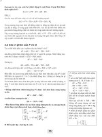
(18) 1.3 Classical Space-Time Transformations. Vg 5 mgy,. 9. (1.23). y op r C fo n d se tio se l U ua en a al ic ion Ev ot L uct N str In. since it can be shown that the work done on or by a body is equivalent to the change in mechanical energy of the body. Although there are a number of other fundamental principles, concepts, and deﬁning equations of classical mechanics that will be utilized in this textbook, those presented in the review will more than satisfy our needs for the next few chapters. A review of a general physics textbook of the deﬁning equations, deﬁned and derived units, basic SI units, and conAuthor ventional symbols for fundamental quantities of classical physics might ISBN # Modern Physics 978097131346 be prudent. Appendix A contains a review of the mathematics (symbols, Fig. # Document name F01-01 31346_F0101.eps algebra, trigonometry, and calculus) necessary for a successful study of Artist Date 11/01/2009 intermediate level modern physics. Accurate Art, Inc.. BxW. 2/C. Check if revision. Author's review (if needed). O Initials. CE's review. O. 4/C. Final Size (Width x Depth in Picas). 16w x 22d. 1.3 Classical Space-Time Transformations. Initials. The classical or Galilean-Newtonian transformation equations for space and time are easily obtained by considering two inertial frames of reference, similar to the coordinate system depicted in Figure 1.1. An inertial Y. P. r. y X z x. Z. Figure 1.1 The position of a particle speciﬁed by a displacement vector in Cartesian coordinates..

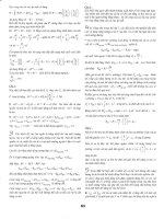
(19) 10. Ch. 1 Classical Transformations. y op r C fo n d se tio se l U ua en a al ic ion Ev ot L uct N str In. frame of reference can be thought of as a nonaccelerating coordinate system, where Newton’s laws of motion are valid. Further, all frames of reference moving at a constant velocity relative to an inertial one are themselves inertial and in principle equivalent for the formation of physical laws. Consider two inertial systems S and S9, as depicted in Figure 1.2, that are separating from one another at a constant speed u. We consider theISBN # Author Modern axis of relative motion between S and S9 to coincide with their Physics respective 978097131346 Fig. # Document name X, X9 axis and that their origin of coordinates coincided at time t 531346_F0102.eps t9 ; 0. F01-02 Generality is not sacriﬁced by regarding system S as being Artist at rest and sysDate 12/14/200 Accuratespeed Art, Inc.u reltem S9 to be moving in the positive X direction with a uniform Check if revision ative to S. Further, the uniform separation of two systems need be BxW 2/C not 4/C along their common X, X9 axes. However, they can be Final so chosen Size (Width xwithout Depth in Picas) x 25d any loss in generality, since the selection of an origin of22w coordinates and the orientation of the coordinate axes in each system is entirely arbitrary. This requirement essentially simpliﬁes the mathematical details, while maximizing the readability and understanding of classical and Einsteinian relativistic kinematics. Further, the requirement that S and S9 coincide at a time deﬁned to be zero means that identical clocks in the two systems. Y. Y9. u. P. y = y9. ut. X, X 9. x9. x. (a) a.. Y. Y9. u. Figure 1.2 The classical coordinate transformations from (a) S to S9 and (b) S9 to S.. P9. y9 = y. ut9. (b) b.. x9 x. X 9, X.

(20) 1.3 Classical Space-Time Transformations. y op r C fo n d se tio se l U ua en a al ic ion Ev ot L uct N str In. are started simultaneously at that instant in time. This requirement is essentially an assumption of absolute time, since classical common sense dictates that for all time thereafter t 5 t9. Consider a particle P (P9 in S9) moving about with a velocity at every instant in time and tracing out some kind of path. At an instant in time t 5 t9 . 0, the position of the particle can be denoted by the coordinates x, y, z in system S or, alternatively, by the coordinates x9, y9, z9 in system S9, as illustrated in Figure 1.2. The immediate problem is to deduce the relation between these two sets of coordinates, which should be clear from the ﬁgure. From the geometry below the X-X9 axis of Figure 1.2a and the assumption of absolute time, we have x9 5 x 2 ut, y9 5 y, z9 5 z, t9 5 t,. (1.24a) (1.24b) (1.24c) (1.24d). S → S9. for the classical transformation equations for space-time coordinates, according to an observer in system S. These equations indicate how an observer in the S system relates his coordinates of particle P to the S9 coordinates of the particle, that he measures for both systems. From the point of view of an observer in the S9 system, the transformations are given by x 5 x9 1 ut9, y 5 y9, z 5 z9, t 5 t9,. (1.25a) (1.25b) (1.25c) (1.25d). where the relation between the x and x9 coordinates is suggested by the geometry below the X9-axis in Figure 1.2b. These equations are just the inverse of Equations 1.24 and show how an observer in S9 relates the coordinates that he measures in both systems for the position of the particle at time t9. These sets of equations are known as Galilean transformations. The space-time coordinate relations for the case where the uniform relative motion between S and S9 is along the Y-Y9 axis or the Z-Z9 axis should be obvious by analogy. The space-time transformation equations deduced above are for coordinates and are not appropriate for length and time interval calculations. For example, consider two particles P1 (P91) and P2 (P92) a ﬁxed distance y 5 y9 above the X-X9 axis at an instant t 5 t9 . 0 in time. The horizontal coordinates of these particles at time t 5 t9 are x1 and x2 in systems S and x91 and x92 in system S9. The relation between these four coordinates, according to Equation 1.24a, is. S9 → S. 11.

(21) 12. Ch. 1 Classical Transformations. x91 5 x1 2 ut, x92 5 x2 2 ut, The distance between the two particles as measured with respect to the S9 system is x92 2 x91. Thus, from the above two equations we have x92 2 x91 5 x2 2 x1,. (1.26). y op r C fo n d se tio se l U ua en a al ic ion Ev ot L uct N str In. which shows that length measurements made at an instant in time are invariant (i.e., constant) for inertial frames of reference under a Galilean transformation. Equations 1.24, 1.25, and 1.26 are called transformation equations because they transform physical measurements from one coordinate system to another. The basic problem in relativistic kinematics is to deduce the motion and path of a particle relative to the S9 system, when we know the kinematics of the particle relative to system S. More generally, the problem is that of relating any physical measurement in S with the corresponding measurement in S9. This central problem is of crucial importance, since an inability to solve it would mean that much of theoretical physics is a hopeless endeavor.. 1.4 Classical Velocity and Acceleration Transformations. In the last section we considered the static effects of classical relativity by comparing a particle’s position coordinates at an instant in time for two inertial frames of reference. Dynamic effects can be taken into account by considering how velocity and acceleration transform between inertial systems. To simplify our mathematical arguments, we assume all displacements, velocities, and accelerations to be collinear, in the same direction, and parallel to the X-X9 axis of relative motion, Further, systems S and S9 coincided at time t 5 t9 ; 0 and S9 is considered to be receding from S at the constant speed u. Our simpliﬁed view allows us to deduce the classical velocity transformation equation for rectilinear motion by commonsense arguments. For example, consider yourself to be standing at a train station, watching a jogger running due east a 5 m/s relative to and in front of you. Now, if you observe a train to be traveling due east at 15 m/s relative to and behind you, then you conclude that the relative speed between the jogger and the train is 10 m/s. Because all motion is assumed to be collinear and in the same direction, the train must be approaching the jogger with a relative.

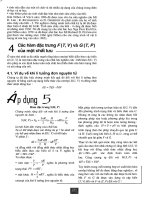
(22) 13. 1.4 Classical Velocity and Acceleration Transformations. velocity of 10 m/s due east. A commonsense interpretation of these velocities (speeds and corresponding directions) can easily be associated with the symbolism adopted for our two inertial systems. From your point of view, you are a stationary observer in system S, the jogger represents an observer in system S9, and the train represents a particle in rectilinear motion. Consequently, a reasonable symbolic representation of the observed velocities would be u 5 5 m/s, vx 5 15 m/s, and v9x 5 10 m/s, which would obey the mathematical relation v9x 5 vx 2 u.. y op r C fo n d se tio se l U ua en a al ic ion Ev ot L uct N str In. (1.27). This equation represents the classical or Galilean transformation of velocities and is expressed as a scalar equation, because of our simplifying assumptions on rectilinear motion. Author ISBN # 978097131346 Modern Physics used For those not appreciating the above commonsense arguments Fig. # Document name for obtaining velocity transformation equation, perhaps the following F01-03 31346_F0103.eps quantitative derivation will be more palatable. Consider the situation Artist Datein12/14/2009 Art, Inc. dicated in Figure 1.3, where a particle is moving in theAccurate X-Y plane for some Check if revision reasonable time interval D t 5 Dt9. As the particle moves from2/Cposition P1 BxW 4/C at time t1 to position P2 at time t2, its rectilinear displacement is measured Final Size (Width x Depth in Picas) by an observer in S to be x2 2 x1. According to this observer, 20w x 19d this distance is also given by his measurements of x92 1 u (t2 2 t1) 2 x91, as suggested in Figure 1.3. By comparing these two sets of measurements, the observer in system S concludes that x92 2 x91 5 x2 2 x1 2 u(t2 2 t1) Y 9(t19 ). Y. Author's review (if needed) OK Initials. OK. Initials. (1.28). u. P1(t1). P2(t2). X, X 9. ut1 ut2 u(t2 – t1). x92. x91 x2 – x1. x1 x2. Date. CE's review. Y9(t29 ). u. Co. Figure 1.3 The displacement geometry of a particle at two different instants t1 and t2, as viewed by an observer in system S.. Date. Co.

(23) 14. Ch. 1 Classical Transformations. for distance traveled by the particle in the S9 system. It should be noted that for classical systems a displacement occurring over a nonzero time interval in not invariant, although previously we found that a length measurement made at an instant in time was invariant. Also, since the time interval for the particle’s rectilinear displacement is t92 2 t91 5 t2 2 t1,. (1.29). y op r C fo n d se tio se l U ua en a al ic ion Ev ot L uct N str In. the division of Equation 1.28 by the time interval equation yields the expected velocity transformation given in Equation 1.27. This result is also easily produced by considering the coordinate transformations given by Equations 1.24a and 1.24d for the two positions of the particle in space and time. Further, the generalization to three-dimensional motion, where the particle has x, y, and z components of velocity, should be obvious from the classical space-time transformation equations. The results obtained for the Galilean velocity transformations in three dimensions are. S → S9. v9x 5 vx 2 u, v9y 5 vy , v9z 5 vz .. (1.30a) (1.30b) (1.30c). Observe that the y- and z- components of the particle’s velocity are invariant, while the x-components, measured by different inertial observers, are not invariant under a transformation between classical coordinate systems. We shall later realize that the y- and z- components of velocity are observed to be the same in both systems because of our commonsense assumption of absolute time. Further, note that the velocities expressed in Equations 1.30a to 1.30c should be denoted as average velocities (e.g., v·9x, v ·x,etc), because of the manner in which the derivations were performed. However, transformation equations for instantaneous velocities are directly obtained by taking the ﬁrst order time derivative of the transformation equations for rectangular coordinates (Equations 1.24a to 1.24c). Clearly, the results obtained are identical to those given in Equations 1.30a to 1.30c, so we can consider all velocities in theses equations as representing either average or instantaneous quantities. Further, a similar set of velocity transformation equations could have been obtained by taking the point of view of an observer in system S9. From Equations 1.25a through 1.25d we obtain. S9 → S. vx 5 v9x 1 u, vy 5 v9y , vz 5 v9z ,. (1.31a) (1.31b) (1.31c).

(24) 1.4 Classical Velocity and Acceleration Transformations. which are just the inverse of Equations 1.30a to 1.30c. To ﬁnish our kinematical considerations, we consider taking a ﬁrst order time derivative of Equations 1.30a through 1.30c or Equations 1.31a through 1.31c. The same results a9x 5 ax , a9y 5 ay , a9z 5 az. (1.32a) (1.32b) (1.32c). y op r C fo n d se tio se l U ua en a al ic ion Ev ot L uct N str In. are obtained, irrespective of which set of velocity transformation equations we differentiate. These three equations for the components of acceleration are more compactly represented by a9 5 a,. (1.33). which indicates acceleration is invariant under a classical transformation. Whether a and a9 are regarded as average or instantaneous accelerations is immaterial, as Equations 1.33 is obtained by either operational derivation. At the beginning of our discussion of classical transformations, we stated that an inertial frame of reference is on in which Newton’s laws of motion are valid and that all inertial systems are equivalent for a description of physical reality. It is immediately apparent from Equation 1.33 that Newton’s second law of motion is invariant with respect to a Galilean transformation. That is, since classical common sense dictates that mass is an invariant quantity, or m9 5 m. (1.34). for the mass of a particle as measured relative to system S9 or S, then from Equations 1.33 and 1.17 we have F9 5 F.. (1.35). Thus, the net external force acting on a body to cause its uniform acceleration will have the same magnitude and direction to all inertial observers. Since mass, time, acceleration, and Newton’s second law of motion are invariant under a Galilean coordinate transformation, there is no preferred frame of reference for the measurement of these quantities. We could continue our study of Galilean-Newtonian relativity by developing other transformation equations for classical dynamics (i.e., mo-. 15.

(25) 16. Ch. 1 Classical Transformations. mentum, kinetic energy, etc.), but these would not contribute to our study of modern physics. There is, however, one other classical relation that deserves consideration, which is the transformation of sound frequencies. The classical Doppler effect for sound waves is developed in the next section from ﬁrst principles of classical mechanics. An analogous pedagogic treatment for electromagnetic waves is presented in Chapter 3, with the inclusion of Einsteinian relativistic effects. As always, we consider only inertial systems that are moving relative to one another at a constant speed.. y op r C fo n d se tio se l U ua en a al ic ion Ev ot L uct N str In 1.5 Classical Doppler Effect. It is of interest to know how the frequency of sound waves transforms between inertial reference frames. Sound waves are recognized as longitudinal waves and, unlike transverse light waves, they require a material medium for their propagation. In fact the speed of sound waves depends strongly on the physical properties (i.e., temperature, mass density, etc.) of the material medium through which they propagate. Assuming a uniform material medium, the speed of sound, or the speed at which the waves propagate through a stationary material medium, is constant. The basic relation vs 5 ln,. (1.36). requires that the product of the wavelength l and frequency n of the waves be equal to their uniform speed vs of propagation. Classical physics requires that the relation expressed by Equation 1.36 is true for all observers who are at rest with respect to the transmitting material medium. That is, once sound waves have been produced by a vibrating source, which can either be at rest or moving with respect to the propagating medium, the speed of sound measured by different spatial observers will be identical, provided they are all stationary with respect to and in the same uniform material medium. Certainly, the measured values of frequency and wavelength in a system that is stationary with respect to the transmitting medium need not be the same as the measured values of frequency and wavelength in a moving system. In this section the unprimed variable (e.g., x, t, l, etc.) are associated with an observer in the receiver R system while the primed variables (e.g., x9, t9, etc.) are associated with the source of sound or emitter E9 system. In all cases the transmitting material medium, assumed to be air, is considered to be stationary, whereas the emitter E9 and receiver R may be either stationary or moving, relative to the transmitting medium. For the situa-.

(26) 1.5 Classical Doppler Effect. y op r C fo n d se tio se l U ua en a al ic ion Ev ot L uct N str In. tion where the receiver R is stationary with respect to air, and the emitter E9 is receding or approaching the receiver, the speed of sound vs as perceived by R is given by Equation 1.36. To deduce the classical frequency transformation, consider the emitter E9 of sound waves to be positioned at the origin of coordinates of the S9 reference frame. Let the sound waves be emitted in the direction of the receiver R, which is located at the origin of coordinates of the unprimed system and is stationary with respect to air. This situation, depicted in Figure 1.4, corresponds to the case where the emitter and detector recede from each other with a uniform speed u. In ﬁgure 1.4 the wave pulses of the emitted sounds are depicted by arcs. It should be noted that the ﬁrst wave pulse received at R occurs at a time D t after the emitter E9 was activated (indicated by the dashed Y9-axis in the ﬁgure). The emitter E9 can be thought of as being activated by pulse of light from R at a time t1 5 t91. A continuous emission of sound waves traveling at approximately 330 m/s is assumed until the ﬁrst sound wave is perceived by R at time t2 5 t92. As Author ISBN # illustrated in Figure 1.4, E9 has moved through the distance uDt during Modern Physics 978097131346 the distance vs the time t2 2 t1 required for the ﬁrst sound wave to travel Fig. # Document name (t2 2t1) to R. When R detects the ﬁrst sound wave, it transmits pulse F01-04 a light 31346_F0104.eps Date traveling at a constant speed of essentially 3 3 108 m/sArtist to E9, thereby stop12/14/2009 Accurate Art, Inc. Check if revision ping the emission of sound waves almost instantaneously. Consequently, BxW 2/CDt9 5 4/CDt the number of wave pulses N9 emitted by E9 in the time interval Final Size (Width x Depth in Picas) is exactly the number of wave pulses N that will be perceived eventually by 18w x 13d R. With x being deﬁned as the distance between R and E9 at that instant in time when R detects the very ﬁrst sound wave emitted by E9, we have l5. x, N. Nth Pulse emitted E9. vsDt. E9 uDt. x. Initials. X, X 9. Date. CE's review OK. Initials. u. 1st Pulse emitted. R. OK. Y 9(t29) u. 1st Pulse received. Author's review (if needed). (1.37). Y9(t19). Y. 17. Figure 1.4 An emitter E9 of sound waves receding from a detector R, which is stationary with respect to air. E9 is activated at time t91 and deactivated at time t92, when R receives the ﬁrst wave pulse.. Date.

(27) 18. Ch. 1 Classical Transformations. where l is the wavelength of the sound waves according to an observer in the receiving system. Solving Equation 1.36 for n and substituting from Equation 1.37 gives n5. vs N x. (1.38). for the frequency of sound waves as observed in system R.. y op r C fo n d se tio se l U ua en a al ic ion Ev ot L uct N str In From Figure 1.4. x 5 (vs 1 u) Dt,. (1.39). thus Equation 1.38 can be rewritten as. vs N . ^vs 1 uh Dt. (1.40). N 5 N9 5 n9 Dt9. (1.41). n5. Substituting. into Equation 1.40 and using the Greek letter kappa (k) to represent the ratio u/vs, u, vs. (1.42). n9 , 11k. (1.43). k;. we obtain the relation. E9 receding from R. n5. where the identity Dt 5 Dt9 has been utilized. Since the denominator of Equation 1.43 is always greater than one (i.e., 1 1 k . 1), the detected frequency n is always lower than the emitted or proper frequency n9 (i.e., n , n9). With musical pitch being related to frequency, in a subjective sense, then this phenomenon could be referred to as a down-shift. To appreciate the rationale of this reference terminology, realize that as a train recedes from you the pitch of its emitted sound is noticeably lower than when it was approaching. The appropriate wavelength transformation is obtained by using Equation 1.36 with Equation 1.43 and is of the form.

(28) 19. 1.5 Classical Doppler Effect. l5. vs ^1 1 kh ; l9^1 1 kh . n9. (1.44). y op r C fo n d se tio se l U ua en a al ic ion Ev ot L uct N str In. Since 1 1 k . 1, l . l9 and there is a shift to larger wavelengths when an emitter E9 of sound waves recedes from an observer R who is stationary with respect to air. What about the case where the emitter is approaching a receiver that is stationary with respect to air? We should expect the sound waves to be bunched together, thus resulting in an up-shift phenomenon. To quantitatively develop the appropriate transformation equations for the frequency and wavelength, consider the situation as depicted in Figure 1.5. Again, let the emitter E9 be at the origin of coordinates of the primed reference system and the receiver R at the origin of coordinates of the unprimed system. As viewed by observers in the receiving system R, a time interval Dt 5 t2 2t1 5 t92 2 t91 is required for the very ﬁrst wave pulse emitted by E9 to reach the receiver R, at which time the emission by E9 is terminated. During this time interval the emitter E9 has moved a distance uDt closer Author ISBN # to the receiver R. Hence, the total numberModern of wavePhysics pulses N9,978097131346 emitted by # name E9 in the elapsed time Dt9, will be bunched Fig. together inDocument the distance x, as ilF01-05 31346_F0105.eps lustrated in Figure 1.5. By comparing this situation with the previous one, Artist Date 11/23/2009 we ﬁnd that Equation 1.37 and 1.38 are stillAccurate valid. Art, ButInc. now,Check if revision BxW. 2/C. Author's review (if needed). Initials. Correx. Date. CE's review. 4/C. x 5 (vs 2 u) Dt Final Size (Width x Depth in Picas). OK. OK. Correx. (1.45). 18w x 13d. Initials. Date. and substitution into Equation 1.38 yields n5. vs N . ^vs 2 uh Dt Y 9(t29). Y. Y 9(t19). u. u. Nth Pulse emitted. 1st Pulse received R. E9 vsDt. 1st Pulse emitted E9. uDt. x. (1.46). X, X 9. Figure 1.5 An emitter E9 of sound waves approaching a detector R, which is stationary with respect to air. E9 is activated at time t91 and deactivated at time t92, at the instant when R receives the ﬁrst wave pulse..

(29) 20. Ch. 1 Classical Transformations. Using Equation 1.41 and 1.42 with Equation 1.46 results in n5. E9 approaching R. n9 . 12k. (1.47). Since 1 2 k , 1, n . n9 and we have an up-shift phenomenon. Utilization of Equation 1.36 will transform Equation 1.47 from the domain of frequencies to that of wavelengths. The result obtained is l 5 l9 (1 2 k),. y op r C fo n d se tio se l U ua en a al ic ion Ev ot L uct N str In. E9 approaching R. (1.48). where, obviously, l , l9 , since 1 2 k , 1. In the above cases the receiver R was considered to be stationary with respect to the transmitting material medium. If, instead the source of the sound waves is stationary with respect to the material medium, then the transformation equations for frequency and wavelength take on a slightly different form. To obtain the correct set of equations, we need only perform the following inverse operations: n → n9. n9 → n. u → 2u .. (1.49). Using these operations on Equation 1.43 and 1.47 gives. R receding from E9 R approaching E9 and. n 5 n9(1 2 k) n 5 n9(1 1 k),. (1.50) (1.51). respectively. In the last two equations the receiver R is considered to be moving with respect to the transmitting medium of sound waves, while the emitter E9 is considered to be stationary with respect to the transmitting material medium. In all cases discussed above, n9 always represents the natural or proper frequency of the sound waves emitted by E9 in one system, while n represents an apparent frequency detected by the receiver R in another inertial system. Clearly, the apparent frequency can be any one of four values for know values of n9, vs, and u, as given by Equations 1.43, 1.47, 1.50, and 1.51. For those wanting to derive Equation 1.50, you need only consider the situation as depicted in Figure 1.6. In this case the ﬁrst wave pulse is perceived by R at time t1, at which time the emission from E9 is terminated. R recedes from E9 at the constant speed u while counting the N9 wave pulses. At time t2 the last wave pulse emitted by E9 is detected by R and of course N 5 N9. Since the material medium is at rest with respect to E9..

(30) 1.5 Classical Doppler Effect Y (t1). Y9. Y (t2 ) u. Nth Pulse emitted. u. R. X 9, X. y op r C fo n d se tio se l U ua en a al ic ion Ev ot L uct N str In. R. Figure 1.6 A detector R of sound waves receding from an emitter E9, which is stationary with respect to air. E9 is deactivated at time t1, when R perceives the ﬁrst wave pulse. R receives the last wave pulse at a later time t2.. Nth Pulse received. 1st Pulse received. E9. 21. x9. uDt9. vs Dt9. vs 5 l9n9.. (1.52). Solving this equation for n9 and using l9 5. and we obtain. x9 N9. x9 5 (vs 2 u)Dt9,. n9 5. (1.53) (1.54). vs N9 . ^vs 2 uh Dt9. Realizing that. N9 5 N 5 nDt. (1.55). and, of course, Dt 5 Dt9, we have the sought after result n 5 n9(1 2 k),. (1.50) R receding from E9. where Equation 1.42 has been used. A similar derivation can be employed to obtain the frequency transformation represented by Equation 1.51..

(31) 22. Ch. 1 Classical Transformations. The wavelength l detected by R when R is receding from E9 is directly obtained by using Equation 1.50 and the fact that the speed of sound waves, as measured by R, is given by R receding from E9. v 5 vs 2 u 5 ln.. (1.56). Solving Equation 1.56 for the wavelength and substituting from Equation 1.50 for the frequency yields vs 2 u , n9^1 2 kh. y op r C fo n d se tio se l U ua en a al ic ion Ev ot L uct N str In l5. (1.57). which, in view of Equation 1.42, immediately reduces to l5. vs . n9. (1.58). Clearly, from Equations 1.52 and 1.58 we have. R receding from E9. l 5 l9.. (1.59). This same result is obtained for the case where R is approaching the stationary emitter E9. By using Equation 1.51 and 1.52 and realizing that the speed of the sound waves as measured by R is given by. R approaching E9. v 5 vs 1 u 5 ln,. (1.60). then we directly obtain the result. R approaching E9. l 5 l9.. (1.61). In each of the four cases presented either the receiver R or the emitter E9 was considered to be stationary with respect to air, the assumed transmitting material medium for sound waves. Certainly, the more general Doppler effect problem involves an emitter E9 and a receiver R both of which are moving with respect to air. Such a problem is handled by considering two of our cases separately for its complete solution. For example, consider a train traveling at 30 m/s due east relative to air, and approaching an eastbound car traveling 15 m/s relative to air. If the train emits sound of 600 Hz, ﬁnd the frequency and wavelength of the sound to observers.

(32) 1.5 Classic Doppler Effect. Y9. 23. Y u = 30 m/s n 9 = 600 Hz. u = 15 m/s. Stationary air •. Train. Car. X, X 9. y op r C fo n d se tio se l U ua en a al ic ion Ev ot L uct N str In. A. Figure 1.7 An emitter (train) and a receiver (car) of sound waves, both moving with respect to stationary air.. in the car for a speed of sound of vs = 330 m/s. This situation is illustrated in Figure 1.7, where the reference frame of the train is denoted as the primed system and that of the car as the unprimed system. To employ the equations for one of our four cases, we must have a situation where either E9 or R is stationary with respect to air. In this example, we simply consider a point, such as A in Figure 1.7, between the emitter (the train) and the receiver (the car), that is stationary with respect to air. This point becomes the receiver of sound waves from the train and the emitter of sound waves to the observers in the car. In the ﬁrst consideration, the emitter E9 (train) is approaching the receiver R (point A) and the frequency is determined by n5. n9 600 Hz 5 5 660 Hz . 30 12k 12 330. Since the receiver R (point A) is stationary with respect to air, then the wavelength is easily calculated by l5. vs 330 m/s 5 5 0.5 m . n 660 Hz. Indeed, the train’s sound waves at any point between the train and the car have a 660 Hz frequency and a 0.5 m wavelength. Now, we can consider point A as the emitter E9 of 660 Hz sound waves to observers in the receding car. In this instance R is receding from E9, thus n 5 n9^12 kh 5 ^660 Hzhc1 2. 15 m 5 630 Hz . 330.

(33) 24. Ch. 1 Classical Transformations. The wavelength is easily obtained, since for this case (R receding from E9) l 5 l9 5 0.5 m. Alternatively, the wavelength could be determined by l5. 330 m/s 2 15 m/s 5 0.5 m , 630 Hz. y op r C fo n d se tio se l U ua en a al ic ion Ev ot L uct N str In. 5. vs 2 u n. since observers in the car are receding from a stationary emitter (point A) of sound waves. The passengers in the car will measure the frequency and wavelength of the train’s sound waves to be 630 Hz and 0.5 m, respectively. It should be understood that the velocity, acceleration, and frequency transformations are a direct and logical consequence of the space and time transformations. Therefore, any subsequent criticism of Equations 1.24a through 1.24d will necessarily affect all the aforementioned results. In fact there is an a priori criticism available! Is one entitled to assume that what is apparently true of one’s own experience, is also absolutely, universally true? Certainly, when the speeds involved are within our domain of ordinary experience, the validity of the classical transformations is easily veriﬁed experimentally. But will the transformation be valid at speeds approaching the speed of light? Since even our fastest satellite travels approximately at a mere 1/13,000 the speed of light, we have no business assuming that v9x 5 vx 2 u for all possible values of u. Our common sense (which a philosopher once deﬁned as the total of all prejudices acquired by age seven) must be regarded as a handicap, and thus subdued, if we are to be successful in uncovering and understanding the fundamental laws of nature. As a last consideration before studying Einstein’s theory on relative motion, we will review in the next section some historical events and conceptual crises of classical physics that made for the timely introduction of a consistent theory of special relativity.. 1.6 Historical and Conceptual Perspective The classical principle of relativity (CPR) has always been part of physics (once called natural philosophy) and its validity seems fundamental, unquestionable. Because it will be referred to many times in this section, and.

(34) 25. 1.6 Historical and Conceptual Perspective. because it is one of the two basic postulates of Einstein’s developments of relativity, we will deﬁne it now by several equivalent statements:. y op r C fo n d se tio se l U ua en a al ic ion Ev ot L uct N str In. 1. The laws of physics are preserved in all inertial frames of reference. 2. There exists no preferred reference frame as physical reality contradicts the notion of absolute space. 3. An unaccelerated person is incapable of experimentally determining whether he is in a state of rest or uniform motion—he can only perceive relative motion existing between himself and other objects. The last statement is perhaps the most informative. Imagine two astronauts in different spaceships traveling through space at constant but different velocities relative to the Earth. Each can determine the velocity of Author ISBN # the other relative to his system. But, neither astronaut can determine, by 978097131346 Modern Physics Fig.is # in a state Document name any experimental measurement, whether he of absolute rest or F01-08 31346_F0108.eps uniform motion. In fact, each astronaut will consider himself at rest and Artist Date 11/20/2009 the other as moving. When you think about it, the classical principle of Accurate Art, Inc. Check if revision relativity is surprisingly subtle, yet it is completely in accord with common BxW 2/C 4/C sense and classical physics. Final Size (Width x Depth in Picas) The role played by the classical principle 28w xof 17drelativity in the crises of theoretical physics that occurred in the years from 1900 to 1905 is schematically presented in Figure 1.8. Here, the relativistic space-time transformations (RT) were developed in 1904 by H.A. Lorentz, and for now we will. Author's review (if needed). Initials. OK. Correx. Date. CE's review. Initials. OK. Correx. Date. Classical Physics. (NM). Theory of Mechanics (Galileo & Newton). Electromagnetic Theory (E&M) (Maxwell). Thermodynamics. must obey the (CPR). Classical Principle of Relativity. (CPR). which employs either. (CT). Classical Space-Time Transformations (Galileo & Newton). or Relativistic Space-Time Transformations (Lorentz & Einstein). (RT). Figure 1.8 Theoretical physics at the turn of the 20th century..

(35) 26. Ch. 1 Classical Transformations. simply accept it without elaborating. There are four points that should be emphasized about the consistency of the mathematical formalism suggested in Figure 1.8. Using the abbreviations indicated in Figure 1.8, we now assert the following: 1. 2. 3. 4.. NM obeys the CPR under the CT. E&M does not obey the CPR under the CT. E&M obeys the CPR under the RT. NM does not obey the CPR under the RT.. y op r C fo n d se tio se l U ua en a al ic ion Ev ot L uct N str In. The ﬁrst statement asserts that NM, the CPR, and the CT are all compatible and in agreement with common sense. But the second statement indicates that Maxwell’s equations are not covariant (invariant in form) when subjected to the CPR and the CT. New terms appeared in the mathematical expression of Maxwell’s equations when they were subjected to the classical transformations (CT). These new terms involved the relative speed of the two reference frames and predicted the existence of new electromagnetic phenomena. Unfortunately, such phenomena were never experimentally conﬁrmed. This might suggest that the laws of electromagnetism should be revised to be covariant with the CPR and the CT. When this was attempted, not even the simplest electromagnetic phenomena could be described by the resulting laws. Around 1903 Lorentz, understanding the difﬁculties in resolving the problem of the ﬁrst and second statements, decided to retain E&M and the CPR and to replace the CT. He sought to mathematically develop a set of space-time transformation equations that would leave Maxwell’s laws of electromagnetism invariant under the CPR. Lorentz succeeded in 1904, but saw merely the formal validity for the new RT equations and as applicable to only the theory of electromagnetism. During this same time Einstein was working independently on this problem and succeeded in developing the RT equations, but his reasoning was quite different from that of Lorentz. Einstein was convinced that the propagation of light was invariant—a direct consequence of Maxwell’s equations of E&M. The Michelson-Morley experiment, which was conducted prior to this time, also supported this supposition that electromagnetic waves (e.g., light waves) propagate at the same speed c 5 3 3108 m/s relative to any inertial reference frame. One way of maintaining the invariance of c was to require Maxwell’s equations of electromagnetism (E&M) to be covariant under a transformation from S to S9. He also reasoned that such a set of space and time transformation equations should be the correct ones for NM as well as E&M. But, according to the fourth statement, Newtonian mechanics (NM) is incompatible with the principle of.

(36) Review of Fundamental and Derived Equations. y op r C fo n d se tio se l U ua en a al ic ion Ev ot L uct N str In. relativity (CPR), if the Lorentz (Einstein) transformation (RT) is used. Realizing this, Einstein considered that if the RT is universally applicable, and if the CPR is universally true, then the laws of NM cannot be completely valid at all allowable speeds of uniform separation between two inertial reference frames. He was then led to modify the laws of NM in order to make them compatible with the CPR under the RT. However, he was always guided by the requirement that these new laws of mechanics must reduce exactly to the classical laws of Galilean-Newtonian mechanics, when the uniform relative speed between two inertial reference frames is much less than the speed of light (i.e., u ,, c). This requirement will be referred to as the correspondence principle, which was formally proposed by Niels Bohr in 1924. Bohr’s principle simply states that any new theory must yield the same result as the corresponding classical theory, when the domain of the two theories converge or overlap. Thus, when u ,, c, Einsteinian relativity must reduce to the well-established laws of classical physics. It is in this sense, and this sense only, that Newton’s celebrated laws of motion are incorrect. Obviously, Newton’s laws of motion are easily validated for our fastest rocket; however, we must always be on guard against unwarranted extrapolation, lest we predict incorrectly nature’s phenomena.. Review of Fundamental and Derived Equations. A listing of the fundamental and derived equations for sections concerned with classical relativity and the Doppler effect is presented below. Also indicated are the fundamental postulates deﬁned in this chapter.. GALILEAN TRANSFORMATION (S → S9) x9 5 x 2 ut_b b y9 5 y ` z9 5 z b b t9 5 t a vx9 5 vx 2 u_ b v9y 5 vy ` b v9z 5 vz a m9 5 m a9 5 a F9 5 F. Space -Time Transformations. Velocity Transformations. Mass Transformation Acceleration Transformation Force Transformation. 27.

(37) 28. Ch. 1 Classical Transformations. CLASSICAL DOPPLER EFFECT vs 5 ln n5. n9 11k. R stationary. 4. l 5 l9 ^1 1 kh n9 n5 12k 4. E9 approaching R. y op r C fo n d se tio se l U ua en a al ic ion Ev ot L uct N str In. l 5 l9 ^1 2 kh. E9 receding from R. vs 5 l9n9 n 5 n9 ^1 2 kh. E9 stationary. _ b v 5 vs 2 u 5 ln` b l 5 l9 a n 5 n9 ^1 1 kh _b v 5 vs 1 u 5 ln` b l 5 l9 a. R receding from E9. R approaching E9. FUNDAMENTAL POSTULATES. 1. Classical principle of Relativity 2. Bohr’s Correspondence Principle. Problems. 1.1 Starting with the deﬁning equation for average velocity and assuming uniform translation acceleration, derive the equation Dx 5 v1D t 1 1 ⁄2a(Dt)2. Solution: For one-dimensional motion with constant acceleration, average velocity can be expressed as the arithmetic mean of the ﬁnal velocity v2 and initial velocity v1. Assuming motion along the X-axis, we have v;. D x v2 1 v1 5 2 Dt.

(38) Problems. and from the deﬁning equation for average acceleration (Equation 1.9) we obtain v2 5 v1 1 aDt, where the average sign has been dropped. Substitution of the second equation into the ﬁrst equation gives Dx v1 1 aDt 1 v1 , 5 2 Dt. y op r C fo n d se tio se l U ua en a al ic ion Ev ot L uct N str In. which is easily solved for Dx,. Dx 5 v1D t 1 1⁄2 a(D t) 2.. 1.2 Starting with the deﬁning equation for average velocity and assuming uniform translation acceleration, derive an equation for the ﬁnal velocity v2 in terms of the initial velocity v1, the constant acceleration a, and the displacement Dx. Answer:. v 22 5 v 12 1 2aDx. 1.3 Do Problem 1.1 starting with Equation 1.5a and using calculus.. Solution: Dropping the subscript notation in Equation 1.5a and solving it for dx gives dx 5 vdt.. By integrating both sides of this equation and interpreting v as the ﬁnal velocity v2 we have. y. x2. x1. dx 5. y. t = Dt. v2 dt .. 0. Since v2 5 v1 1 at, substitution into and integration of the last equation yields Dx 5. y. 0. ^v1 1 at h dt 5 v1 Dt 1 2 a^Dt h2.. t = Dt. 1. 1.4 Do Problem 1.2 starting with Equation 1.7 and using calculus. Answer:. v 22 5 v 12 1 2aDx. 1.5 Staring with W 5 F ? Dx and assuming translational motion, show that W 5 DT by using the deﬁning equations for average velocity and acceleration.. 29.

(39) 30. Ch. 1 Classical Transformations. Solution: W 5 F ? Dx 5 F cos u Dx. definition of a dot product. 5 F Dx. assu min g u 5 0c. 5 ma Dx. assu min g m ! m (t). 5m. Dv Dx Dt. from Eq. 1.9. Dx Dt v2 1 v1 5 m Dv c m 2. y op r C fo n d se tio se l U ua en a al ic ion Ev ot L uct N str In. 5 m Dv. average velocity definition. 5 2 m^v2 2 v1h^v2 1 v1h 1. 5 2 mv22 2 2 mv12 1. 1. 5 DT. from Equation 1.22. 1.6 Starting with the deﬁning equation for work (Equation 1.20) and using calculus, derive the work-energy theorem. Answer:. W 5 DT. 1.7 Consider two cars, traveling due east and separating from one another. Let the ﬁrst car be moving at 20 m/s and the second car at 30 m/s relative to the highway. If a passenger in the second car measures the speed of an eastbound bus to be 15 m/s, ﬁnd the speed of the bus relative to observers in the ﬁrst car. Solution: Thinking of the ﬁrst car as system S and the second as system S9, then u 5 (30 2 20) m/s 5 10 m/s. With the speed of the bus denoted accordingly as v9x 5 15 m/s, vx is given by Equation 1.30a or Equation 1.31a as vx 5 v9x 1 u 5 15 m/s 1 10 m/s 5 25 m/s.. 1.8 Consider a system S9 to be moving at a uniform rate of 30 m/s relative to system S, and a system S0 to be receding at a constant speed of 20 m/s relative to system S9. If observers in S0 measure the translational speed of a particle to be 50 m/s, what will observers in S9 and S measure for the speed of the particle? Assume all motion to be the positive x-direction.

(40) Problems. along the common axis of relative motion. Answer:. 70 m/s, 100 m/s. y op r C fo n d se tio se l U ua en a al ic ion Ev ot L uct N str In. 1.9 A passenger on a train traveling at 20 m/s passes a train station attendant. Ten seconds after the train passes, the attendant observes a plane 500 m away horizontally and 300 m high moving in the same direction as the train. Five seconds after the ﬁrst observation, the attendant notes the plane to be 700 m away and 450 m high. What are the space-time coordinates of the plane to the passenger on the train? Solution: For the train station attendant x1 5 500 m x2 5 700 m. y1 5 300 m y2 5 450 m. t1 5 10 s t2 5 15 s .. For the passenger on the train. x91 5 x1 2 ut1 5 500 m 2 `20. m j ^10 sh 5 300 m , s. y91 5 y1 5 300 m ,. t91 5 t1 5 10 s ,. x92 5 x2 2 ut2 5 700 m 2 `20. m j ^15 sh 5 400 m , s. y92 5 y2 5 450 m , t92 5 t2 5 15 s .. 1.10 From the results of Problem 1.9, ﬁnd the velocity of the plane as measured by both the attendant and the passenger on the train. Answer:. 50 m/s at 36.9˚, 36.1 m/s at 56.3˚. 1.11 A tuning fork of 660 Hz frequency is receding at 30 m/s from a stationary (with respect to air) observer. Find the apparent frequency and wavelength of the sound waves as measured by the observer for vs 5 330 m/s. Solution: With n9 5 660 Hz and u 5 30 m/s for the case where E9 is receding from R, n5. n9 600 Hz 5 5 605 Hz 12 11k 11. 31.

(41) 32. Ch. 1 Classical Transformations. and. l5. vs 330 m/s 5 5 0.545 m . n 605 Hz. 1.12 Consider Problem 1.11 for the case where the tuning fork is approaching the stationary observer. Answer:. 726 Hz, 0.455 m. y op r C fo n d se tio se l U ua en a al ic ion Ev ot L uct N str In. 1.13 Consider Problem 1.11 for the case where the observer is approaching the stationary tuning fork. Solution: With n9 5 660 Hz and u 5 30 m/s for the case where R is approaching E9, we have. or. 12 n 5 n9 ^1 1 kh 5 660 Hz c m 5 720 Hz , 11 vs 1 u 330 m/s 1 30 m/s 5 5 0.5 m l5 n 720 Hz l 5 l9 5 0.5 m.. 1.14 Draw the appropriate schematic and derive the frequency transformation equation for the case where the emitter E9 is stationary with respect to air and the receiver R is approaching the emitter. Answer:. n 5 n9 (1 1 k). 1.15 Consider Problem 1.11 for the case where the observer is receding from the stationary tuning fork. Solution: Given that n9 5 660 Hz, u 5 30 m/s, vs 5 330 m/s, and R is receding from E9, then. or. 10 n 5 n9 ^1 2 kh 5 660 Hz c m 5 600 Hz , 11 vs 2 u 330 m/s 2 30 m/s 5 5 0.5 m l5 n 600 Hz l 5 l9 5 0.5 m.. 1.16 Consider a train to be traveling at a uniform rate of 25 m/s relative to stationary air and a plane to be in front of the train traveling at 40 m/s relative to and in the same direction as the train. If the engines of the plane produce sound waves of 800 Hz frequency, what is the frequency and wavelength of the sound wave to a ground observer located behind the.

(42) Problems. plane for vs 5 335 m/s. Answer:. 670 Hz, 0.5 m. 1.17 What is the apparent frequency and wavelength of the plane’s engines of Problem 1.16 to passengers on the train?. y op r C fo n d se tio se l U ua en a al ic ion Ev ot L uct N str In. Solution: Any stationary point in air between the plane and the train serves as a receiver of sound waves from the plane and an emitter of sound waves to the passengers on the train. Thus, from the previous problem we have n9 5 670 Hz, l9 5 0.5 m, u 5 25 m/s, and vs 5 335 m/s, where the receiver (train) is approaching the emitter (stationary point). For this case the frequency becomes n 5 n9 ^1 1 kh 5 670 Hz c1 1. 5 m 5 720 Hz 67. and the wavelength is given by l5. vs 1 u 360 5 5 0.5 m n 720. or. l 5 l9 5 0.5 m .. 1.18 A train traveling at 30 m/s due east, relative to stationary air, is approaching an east bound car traveling at 15 m/s, relative to air. If the train emits sound of 600 Hz, ﬁnd the frequency and wavelength of the sound to a passenger in the car for vs 5 330 m/s. Answer:. 630 Hz, 0.5 m. 1.19 A train traveling due west at 30 m/s emits 500 Hz sound waves while approaching a train station attendant. A driver of an automobile traveling due east at 15 m/s and emitting sound waves of 460 Hz is directly approaching the attendant, who is at rest with respect to air. For vs 5 330 m/s, ﬁnd the frequency and wavelength of the train’s sound waves to the driver of the automobile. Solution: From the train to the attendant we have n9 5 500 Hz, u 5 30 m/s, vs 5 330 m/s, and E9 approaching R: n5. n9 500 Hz 5 5 550 Hz , 1 2 k 1 2 1/11. l5. vs 330 m/s 3 5 5 m. n 550 Hz 5. From the attendant to the automobile we have n9 5 550 Hz, u 5 15. 33.

(43) 33a. Ch. 1 Classical Transformations. m/s, vs 5 330 m/s, and R approaching E9: n 5 n9 ^1 1 kh 5 550 Hz c1 1 l 5 l9 5. 3 m 5. or. 1 m 5 575 Hz , 22 vs 1 u 375 3 l5 5 5 m. n 575 5. y op r C fo n d se tio se l U ua en a al ic ion Ev ot L uct N str In. 1.20 After the automobile and train of Problem 1.19 pass the train station attendant, what is the frequency of the automobile’s sound waves to passengers on the train? Answer:. 400 Hz.

(44) 34. CH. A P T E R. 2. Basic Concepts of Einsteinian Relativity. y op r C fo n d se tio se l U ua en a al ic ion Ev ot L uct N str In A depiction of a train traveling with a relativistic velocity as observed from the frame of reference of the train station.. The relativity theory arose from necessity, from serious and deep contradictions in the old theory from which there seemed no escape. The strength of the new theory lies in the consistency and simplicity with which it solves all these difﬁculties, using only a few very convincing assumptions. . . . The old mechanics is valid for small velocities and forms the limiting case of the new one. A. EINSTEIN AND L. INFELD,. The Evolution of Physics (1938). Introduction The discussion of Galilean relativity in the last chapter was mostly in accord with common sense. The results obtained were intuitive and in agreement with everyday experience for inertial systems separating from one another at relatively low speeds. The problems associated with comparing physical measurements made by different inertial observers were easily.

(45) 35. Ch. 2 Basic Concepts of Einsteinian Relativity. y op r C fo n d se tio se l U ua en a al ic ion Ev ot L uct N str In. handled, once the Galilean space-time coordinate transformations were obtained. Central to Galilean relativity was the assumption of absolute time, which suggests that two clocks initially synchronized at t 5 t9 ; 0 will remain synchronized when they are moving relative to one another at a constant speed. A direct consequence of this assumption is that time interval measurements are invariant, Dt 5 Dt9, for observers in different inertial systems, since temporal coordinates would be identical, t 5 t9, for all of time. Thus, simultaneous measurements of two spatial positions at an instant in time results in an invariance of length, Dx 5 Dx9, in Galilean relativity. This chapter is primarily concerned with time interval and length measurements, along with the concepts of synchronization and simultaneity, within the framework of Einstein’s special theory of relativity. Einsteinian relativity is an elegant theory that arises logically and naturally from two fundamental postulates: (1) the classical principle of relativity and (2) the invariance of the speed of light. Like Galilean relativity, Einstein’s theory is concerned with problems involving the comparison of physical measurements made by observers in different inertial frames of reference. It differs signiﬁcantly and fundamentally from Galilean relativity in that the two postulates of relativity are devoid of any temporal assumption. It will be shown that the invariance of time, as well as the invariance of length, must in general be abandoned, when the speed of light is assumed invariant. The results of Galilean relativity for time interval and length measurements are, however, directly obtained from Einsteinian relativity under the correspondence principle, for the situation where the uniform speed of separation between two inertial systems is small compared to the speed of light. Einsteinian relativity has the completely undeserved reputation of being mathematically intimidating and conceptually mystifying to all but a few students. This misconception will be laid to rest in this and the next two chapters, as Einstein’s special theory of relativity is fully developed utilizing only elementary mathematics of algebra, trigonometry, and occasionally introductory calculus. In developing Einsteinian relativity from the two fundamental postulates, gedanken (German for thought) experiments will be utilized in illustrating particular concepts that are not intuitive from everyday experience. Although some concepts will be introduced that are not in accord with common sense and may defy visualization, they will be intellectually stimulating and exciting to the imagination. These new concepts and results present a far reaching and nonclassical view of the intimate relationships between space, time, matter, and energy that is essential for the understanding of microscopic phenomena. Consequently, the study of special relativity is very important for students of contemporary (atomic, nuclear, and solid state, etc.) physics and electrical engineering..

(46) 2.1 Einstein’s Postulates of Special Relativity. 2.1 Einstein’s Postulates of Special Relativity. y op r C fo n d se tio se l U ua en a al ic ion Ev ot L uct N str In. The incompatibility of the laws of electromagnetism, the classical principle of relativity, and the Galilean space-time transformation led Einstein to a critical reevaluation of the concepts of space, time, and simultaneity. He decided to abandon the Galilean transformation of relativity and adopt a more fundamental principle of relativity that would be applicable to all physical laws- electromagnetism and mechanics. Einstein developed the special theory of relativity from the following two fundamental postulates: 1. the classical principle of relativity. 2. the invariance of the speed of light.. Einstein was the ﬁrst to recognize the profound nature and universal applicability of the classical principle of relativity and to raise it to the status of a postulate. This postulate suggests that all physical laws, including those of electromagnetism and mechanics, are covariant in all inertial frames of reference. Not only are the mathematical interrelations of physical laws preserved, but also the values associated with all physical constants are identical in all inertial reference frames. Thus, the notion of an absolute frame of reference is forever discarded, and the concept of invariance is assumed for all of physics. The second postulate is a direct consequence of Maxwell’s equations and a fact resulting from the Michelson-Morley experiment. It is incompatible with the ﬁrst postulate under the Galilean transformation but totally compatible with the classical principle of relativity under the Lorentz transformation, as well be seen in the next chapter. For now, we will attempt to develop an understanding of the physical implications of Einstein’s postulates, by considering some simple and intuitive examples involving two identical luxury vans traveling on a straight smooth road. To elaborate on Einstein’s ﬁrst postulate, consider that you are riding in one of the vans at a constant velocity of 25 m/s due west. You lie back in the captain’s chair against the headrest and feel very comfortable, not experiencing and bumps or accelerations. In fact, if you slump down in the chair and look far out at the horizon, you will not have any physical sensation of motion. Now, let a second identical van, being driven by your brother, approach you from behind at a uniform speed of 30 m/s relative to the ground. When your brother’s van comes into view, you make some measurements and conclude that he is traveling relative to you at 5 m/s due west. On the other hand, if your brother measured your speed, he would conclude that you are backing up toward him with a relative speed of 5 m/s. You and your brother each determine that the other is moving with a relative speed of 5 m/s, but you can not make physical measure-. 36.

(47) 37. Ch. 2 Basic Concepts of Einsteinian Relativity. y op r C fo n d se tio se l U ua en a al ic ion Ev ot L uct N str In. ments that would determine whether you are moving, he is moving, or both of you are moving. This result is consistent with the classical principle of relativity and carries over to all possible physical measurements in each van. Further, the results of an experiment performed on any physical system on your van must yield identical numerical results to those obtained by your brother, when he conducts the same experiment on an identical system in his van. For example, if you measure the frequency of sound waves produced by your van’s horn to be 550 Hz, then your brother would measure the fundamental frequency of sound from his van’s horn to be 550 Hz. Also, you would measure the speed of light from your van’s dome light to be 3 3 108 m/s (approximately) and your brother would obtain the same result for the speed of light from his van’s dome light. What about the situation where you measure the frequency of sound produced by your brother’s horn and he measures the frequency of sound from your horn? From the results of the classical Doppler effect in the last chapter, you know the two frequency measurements will be dissimilar, since your brother is approaching and you are receding from sound waves in stationary air. The relative speed between the sound waves in air and your brother would be vs 1 30 m/s, while it would be vs 2 25 m/s between the sound in air and you. In this situation the transporting material medium (air) for sound waves is another frame of reference in addition to the reference frames of the two vans. What about the situation where you measure the speed of light from your brother’s headlights and he measures the speed of light from your taillights? Unlike sound waves, light does not require any material medium for its transmission, and you need only consider your frame of reference and that of your brother. In this case the two vans are viewed as approaching each other with a constant speed of u 5 5 m/s. As such, common sense dictates that the relative speed between you and the light from your brother’s headlights would be c 1 u and, likewise, between your brother and the light from your taillights. Although this result is intuitive and in agreement with Galilean relativity, it is not consistent with Einstein’s second postulate. According to Einstein, you and your brother would measure the relative speed to be c 5 3 3 108 m/s, since the speed of light is invariant and independent of the relative motion between the source and observer. To emphasize this point, suppose your bother’s van is overtaking you and at half the speed of light and after he passes, you ﬂash your headlights at him (possibly to indicate to him that in your considered opinion he is violating a trafﬁc law). Einstein’s second postulate predicts that he would measure the speed of light from your headlights to pass him at the normal speed of c 5 3 3 108 m/s! In fact, he would observe the same speed of light for that emitted from your headlights as you would observe, regardless of his speed relative to you. Surely, you must ﬁnd this hard to be-.

(48) 2.2 Lengths Perpendicular to the Axis of Relative Motion. y op r C fo n d se tio se l U ua en a al ic ion Ev ot L uct N str In. lieve and most remarkable. After all, does it not violate our notions of common sense? Yet, every experimental examination of this phenomenon veriﬁes the truth of Einstein’s second postulate. Serious experimental veriﬁcation of Einstein’s second postulate was not possible until the technological advances of the twentieth century. Perhaps because of this, the invariance of light was not realized nor even seriously contemplated, until Einstein published his work on relativity. It was his remarkable insight and understanding that brought about an intellectual and philosophical revolution and made man recognize the limitations of his dimensional experience. If natural phenomena exist that are conceptually beyond the grasp of man’s reasoning—beyond deductive realization or physical veriﬁcation— then we must unshackle our imaginations and arrest our beliefs, if we are to visualize the subtle laws of nature. We will now deduce the basic results of Einstein’s special theory of relativity from some gedanken experiments. As always, we consider two frames of reference, S and S9, to be separating from each other along their common X-X9 axis at the uniform speed u, after having coincided at time t 5 t9 ; 0. Further, it is conceptually convenient to allow observers to exist at many different spatial positions at the same instant in time in both the S and S9 frame of reference. Thus, observers spatially separated and at rest in a particular frame of reference can synchronize their clocks and simplify their measurements of spatial and temporal intervals for a particle (or system) traveling at a relativistic speed.. 2.2 Lengths Perpendicular to the Axis of Relative Motion. As a beginning to the development of Einsteinian relativity from the two fundamental postulates, consider whether coordinate axes that are perpendicular to an axis of relative motion in one frame of reference will be viewed by other inertial observers as being perpendicular. The gedanken experiment for this query is depicted in Figure 2.1, where a meter stick is aligned with the Y-Z plane in system S and another with the Y9-Z9 plane in system S9. At the top of each meter stick is located a small plane mirror, labeled M in system S and M9 in the S9 system, adjusted so the mirror surfaces face each other. At some instant in time, a beam of light is emitted from M parallel to the X-axis at a distance y above it and in the direction of the M9 mirror. How does the beam of light appear to an observer in the S9 frame of reference? For consistency with Einstein’s second postulate, he will view the beam of light as traveling at the uniform speed c and incident on his. 38.

(49) 39. Ch. 2 Basic Concepts of Einsteinian Relativity Y. Y9 u. M9. M. y op r C fo n d se tio se l U ua en a al ic ion Ev ot L uct N str In X, X 9. Figure 2.1 The reﬂection of a light beam between two plane mirrors set up parallel to one another in systems S and S9. Z. Z9. M9 mirror at some distance y9 above his X9 -axis. When the beam of light strikes the M9 mirror, the observer in S9 notices the beam of light is reﬂected upon its incident path concluding that the beam of light is parallel to his X9-axis. This result is consistent with the initial requirements that the X9-axis coincides with the X-axis and that the beam of light was adjusted to be parallel to the X-axis. An observer in system S will also notice the beam of light to be reﬂected from M9 upon its incident path, in accordance with Einstein’s ﬁrst postulate. He concludes that the M9 mirror must have been perpendicular to the beam of light and, thus, M9 must be parallel to his mirror M. The conclusion that the two mirrors are parallel would also be obtained by the observer in S9, if he were to initiate a beam of light from M9 parallel to his X9 axis and in the direction of M. As yet we do not know if y 5 y9, but the observers in both reference frames conclude that the two mirrors are parallel to one another and perpendicular to their common X-X9 axis. Since the mirrors are parallel, then so are the Y-Z and Y9-Z9 planes. Thus, in general, observers in different inertial frames of reference see coordinate axes Y, Y9, Z, Z9 as being perpendicular to the X-X9 axis. Since our systems S and S9 coincided at time t 5 t9 ; 0, in addition to being perpendicular to the axis of relative motion Y is parallel to Y9 and, likewise, Z and Z9 are parallel. In general, this need not be true for inertial systems that are not moving along a common axis; however, all inertial observers having a common axis of relative motion will view any length measurement made perpendicular to their common axis as being normal to that axis..

(50) 2.2 Lengths Perpendicular to the Axis of Relative Motion. y op r C fo n d se tio se l U ua en a al ic ion Ev ot L uct N str In. From the above discussion it is easy to argue that the distance of the light beam above the X-X9 axis is the same for observers in both systems (i.e., y = y9). Obviously, since the light beam strikes M9 and is reﬂected upon its incident path a distance y9 above the X9-axis, the value of y9 measured in S9 must be the same as the value y measured in S. Suppose, however, that the light reﬂected from M9 strikes above the mirror M in system S. An observer in the S frame of reference would surmise that his meter stick was smaller than the meter stick in the S9 frame of reference. But, according to Einstein’s ﬁrst postulate, if an observer in S9 were to send out a beam of light from M9 parallel to the X-X9 axis so as to be reﬂected from M, he would conclude that his meter sick was smaller than the meter stick in system S. As illustrated in Figure 2.1, the two reﬂected rays for this hypothetical case would necessarily cross. However, since light, propagating at a constant velocity, travels in a straight line, parallel incident rays (in our case they are coincident) are reﬂected from parallel plane mirrors such that the reﬂected rays are parallel! Thus, there is a contradiction between Einstein’s ﬁrst and second postulates, which means that our initial supposition is in violation of nature’s law and, therefore, incorrect. According to Einstein’s ﬁrst postulate, any supposition made by an observer in system S would necessarily be the same supposition made by an observer in the S9 frame of reference. If the supposition violates any known laws, like the ﬁrst gedanken experiment or the fact that parallel light rays never cross, then the supposition is wrong. An analogous argument shows the impossibility of a beam of light being emitted from M, parallel to the X-X9 axis, and reﬂected from M9 such as to return below M. Consequently, the only possible conclusion is the one stated initially: any length or coordinate measurement made perpendicular to the axis of relative motion has the same value for all inertial observers. This generalization can be expressed as. and. y9 5 y. Dy9 5 Dy. (2.1). z9 5 z. Dz9 5 Dz,. (2.2). which are two of the three Lorentz space-coordinate transformations. Clearly, these are identical to the Galilean space transformations for the y, y9 and z, z9 coordinates. As yet, we do not know the relativistic spatial transformation for the x, x9 coordinates and we should not, at this time, make any assumptions regarding its form.. 40.

(51) 41. Ch. 2 Basic Concepts of Einsteinian Relativity. 2.3 Time Interval Comparisons In this gedanken experiment, illustrated in Figure 2.2, we let the plane of a mirror M9 be perpendicular to the Y9-axis at some distance Dy9 above the origin of coordinates. An observer in S9 sends a light pulse up the Y9axis, where it is reﬂected upon its incident path by the mirror M9 and eventually absorbed at its point of origin O9. In accordance with Figure 2.2, any S9 observer will measure the distance from O9 to M9 to be given by D t9 1 m 5 2 cD t9 , 2. y op r C fo n d se tio se l U ua en a al ic ion Ev ot L uct N str In. Dy9 5 c c. (2.3). where Dt9 is deﬁned as the time it takes the light pulse to travel from O9 to M9 and back to O9. Observers in the S frame of reference do not see the motion and path of the light pulse in S9 as being vertical, since M9 (at rest relative to S9) is moving at a uniform speed u relative to their reference frame. Instead, they observe the motion and path of the light pulse in S9 to be something like the isosceles triangle depicted in Figure 2.2, where Dt ; tB 2 tA is the time interval, according to S observers, for the light pulse to go from A to M9 to B. It should be obvious that, whereas S9 observers need only one clock to measure the time interval Dt9, S observers need two clocks for their measurement of the corresponding time interval Dt. In system S,. Y9(tA). Y. u. u. u. M9. M9. M9. 1. Dy. Figure 2.2 The path of a vertical pulse of light being reﬂected from a mirror in S9, as viewed by observers in S9 and S.. Dy9. A. Z. Z9. Y9(tB). Y9. t. cD. 1 cDt 9 2. 2. 09. 09 1 2. 09 B. uDt. Z9. Z9. X, X 9.

(52) 2.3 Time Interval Comparisons. we need one clock at A and another at B, and since the two clocks are spatially separated, it is essential that they be synchronized. Later, we will consider a method by which clocks can be synchronized, but for now, we simply assume the synchronization of clocks at A and B has been effected. Clearly, Dt corresponds to the difference between the reading of the two clocks at A and B in system S. Viewing the left triangle of Figure 2.2 and invoking the Pythagorean theorem, we have. y op r C fo n d se tio se l U ua en a al ic ion Ev ot L uct N str In (Dy)2 1 ( 12 uDt)2 5 ( 12 cDt)2,. which is easily solved for Dy in the form 1. Dy 5 2 c Dt 1 2 b2 ,. (2.4). u b; . c. (2.5). where we have set. Here, Dy is the vertical displacement of the mirror M9, as measured by observers in system S. Now, using Equation 2.1 from the previous gedanken experiment (Dy 5 Dy9) along with Equations 2.3 and 2.4, we have 1. 2. By deﬁning. 1. c D t 1 2 b2 5 2 c D t9.. g;. 1. 1 2 b2. (2.6). (2.7). and solving Equation 2.6 for Dt, we obtain Dt 5 gDt9.. (2.8) Time Dilation. The result expressed by Equation 2.8 gives a comparison of time intervals measured in two different inertial reference frames. The meaning and implications of this result may need some elaboration. First, consider that in the limit as u approaches c in Equation 2.7 (remember b 5 u/c), g approaches `. However, for u ,, c, g approaches 1, and Equation 2.8 reduces to the Galilean transformation (Equation 1.29) in accordance with. 42.

(53) 43. Ch. 2 Basic Concepts of Einsteinian Relativity. the correspondence principle. Thus, the range of values for g can be expressed as 1 # g # `,. (2.9). y op r C fo n d se tio se l U ua en a al ic ion Ev ot L uct N str In. which implies that Dt . Dt9 in Equation 2.8 for u not small. That is, the time interval Dt measured between two events (emission and absorption of the light pulse) occurring at spatially different positions in system S is greater than the proper time Dt9, which is the time interval measured in system S9 between two events occurring at the same position. Because of the factor g in Equation 2.8, Dt is greater than the proper time and is referred to as a dilated time. Hence, the name time dilation that is normally associated with Equation 2.8. It is important to keep in mind Einstein’s ﬁrst postulate, because if the experiment were performed in system S, observers in S9 would conclude that Dt9 5 gDt. The signiﬁcance of the time dilation result is that it emphasizes how time interval measurements differ between inertial observers in relative motion, because of differing physical measurements. A time interval between two events is always shortest in a system where the events occur at the same position and dilated by the factor g in all other inertial systems. In solving problems associated with the time dilation equation, it is most convenient and less confusing to identify the proper time as occurring in the primed system, with the dilated time then given by Equation 2.8 for the unprimed inertial system. As the concept of time dilation is most incredible, a few examples will be presented in an attempt to clarify the subtleties of the phenomenon. If you believe the secret of eternal youth is in keeping on the move, you are not far from wrong. In fact, time dilation predicts that if you have a twin, your biological clocks will be different, if one twin is traveling uniformly at a relativistic speed (e.g., u . 0.4c) relative to the other. For example, consider that at age twenty you take off in a rocket ship traveling at 0.866 the speed of light. You leave behind a younger brother of age ten and travel through space for twenty years (according to your clock). When you return home, at age forty, you will ﬁnd your kid brother to be ﬁfty years old! He will have aged by Dt = 40 years, while you have aged by only Dt9 = 20 yrs. That is, time dilation gives Dt 5 gDt9 5 ^20 yrsh / 1 2 ^.866c/ch2 5 40 yrs . As compared to your brother, your biological clock and aging process was slowed by the time dilation effect. It should be emphasized that time dilation is a real effect that applies not just to clocks but to time itself—time ﬂows at different rates to different inertial observers..

(54) 2.4 Lengths Parallel to the Axis of Relative Motion. Other time dilation effects have been observed in laboratories for the lifetimes of radioactive particles. As a particular example, consider the decay of unstable elementary particles called muons (or mu-mesons). A muon is observed in a laboratory to decay into an electron in an average time of 2.20 3 1026 sec, after it comes into being. Normally, muons are created in the upper atmosphere by cosmic ray particles and travel with a uniform mean speed of 2.994 3 108 m/s 5 0.9987c toward the earth’s surface. In their lifetime, the muons should be able to travel a distance of m j ^2.20 3 1026 sh 5 659 m , s. y op r C fo n d se tio se l U ua en a al ic ion Ev ot L uct N str In. s 5 uDt 5 `2.994 3 108. according to the laws of classical kinematics. Since they are created at altitudes exceeding 6000 m, they should rarely reach the earth’s surface. But they do reach the earth’s surface and in profusion—approximately 207 muons per square meter per second are detected at sea level. The muon paradox is immediately resolved, if we take time dilation into account. According to observers in the earth’s reference frame, the muon’s proper mean lifetime is Dt9 5 2.20 3 1026 s. The mean time that we observe the muons in motion is a time dilated to the value Dt 5 g Dt 9 5. 2.20 3 1026 s 0.9987c 2 12 c m c. 5 43.1 3 1026 s .. Thus, according to Einstein’s postulates, the muons should (and do) travel a mean distance of D x 5 u Dt 5 `2.994 3 108. m j ^43.1 3 1026 sh 5 1.29 3 104 m s. in our reference frame.. 2.4 Lengths Parallel to the Axis of Relative Motion Consider the situation schematically illustrated in Figure 2.3, where observers in S9 have placed a mirror M9 perpendicular to their X9-axis at. 44.

(55) 45. Ch. 2 Basic Concepts of Einsteinian Relativity. Y. Y9. u. M9. y op r C fo n d se tio se l U ua en a al ic ion Ev ot L uct N str In. Figure 2.3 A horizontal pulse of light being reﬂected from a vertical mirror in S9, as viewed by observers in S.. A9. X 9, X. Dx95 12 cDt 9. some distance Dx9 from the origin of their reference frame. In order to measure the distance Dx9, they send out a light pulse from A9 parallel to the X9-axis such that it will be reﬂected by M9 back to A9. For generality we will denote this distance by Dx9 and, thus, observers in S9 reason that c5. 2Dx9 , Dt9. where Dt9 is the time interval required for the light pulse to travel A9 to M9 and back to A9. Thus, the distance they measure between A9 and M9 is given by Dx9 5 12 c Dt9,. (2.10). where Dt9 should be interpreted as a length measurement. What do observers in system S measure, and how do they operationally perform the necessary measurements for the length in question? First consider the motion of the light pulse from A9 to M9 as viewed by observers in the S-frame and depicted in Figure 2.4. Observers in system S note the origination of the light pulse at point A at time tA. It propagates to the right at the uniform speed c, while the mirror M9 moves to the right uniformly at a speed u. At some later time tB, the observers in S will note the light pulse striking the mirror M9. The two clocks in S record a time difference of DtA2B ; tB 2 tA and, thus, the light pulse must have traveled the distance cDtA2B. With the distance from the origin of the Y9-axis to the mirror M9 (as measured by S-observers) denoted by Dx, then Figure.

(56) 2.4 Lengths Parallel to the Axis of Relative Motion. Y. Y 9(tA). Y 9(tB) u. u. Figure 2.4 A horizontal pulse of light propagating towards a vertical mirror in S9, as viewed by observers in S.. M9(tB). y op r C fo n d se tio se l U ua en a al ic ion Ev ot L uct N str In. M9(tA). A. 46. uDtA– B. Dx. B. X, X 9. cDtA– B. 2.4 suggest that. Dx 5 (c 2 u)DtA2B.. Thus, the time interval DtA2B is given by DtA2B 5. Dx . c2u. (2.11). Now, consider the motion of the light pulse from M9 back to the Y9axis, as viewed by observers in system S. The situation, as depicted in Figure 2.5, suggests that the light pulse is reﬂected from M9 at point B at the time tB. It then propagates to the left at the speed of light c, arriving at the Y9-axis at point C and time tC. Of course, during the time interval DtB2C 5 tC 2 tB, the S9-frame and mirror M9 were moving to the right with constant speed u. In this case, the distance Dx in question is immediately obtained from Figure 2.5 as Dx 5 (c 1 u) DtB2C. Solving the above equation for the time interval DtB2C gives DtB2C 5. Dx , c1u. (2.12). which is not the same as DtA2B as far as observers in system S are concerned. These results also agree with classical common sense. That is, if.

(57) 47. Ch. 2 Basic Concepts of Einsteinian Relativity. Y. Y 9(tB). Y 9(tC) u. u. y op r C fo n d se tio se l U ua en a al ic ion Ev ot L uct N str In. Figure 2.5 A horizontal pulse of light being reﬂected from a vertical mirror in S9, as viewed by observers in S.. M9(tB). B. C. cDtB – C. M9(tC). uDtB – C. X, X 9. Dx. the mirror and light pulse are traveling to the right, then the relative speed between the light pulse and the mirror is c 2 u and Equation 2.11 is immediately obtained. On the other hand, if the mirror is moving to the right while the light pulse is traveling to the left, then the relative speed of separation between the mirror and the light pulse is c + u, which lead to Equation 2.12. Let observers in S deﬁne the time interval Dt as that time required for the pulse of light in S9 to travel from A9 to M9 and back to A9, as viewed in their reference frame. Clearly, then Dt 5 DtA2B 1 DtB2C 5. Dx Dx , 1 c2u c1u. which, when solved for Dx, yields Dx 5 2 c Dt c1 2 1. u2 . m c2. (2.13). Substitution of Equation 2.8 into Equation 2.13 gives Dx 5 2 c Dt9g ^1 2 b2h , 1. (2.14). where Equation 2.5 has been utilized for b. Now, from Equation 2.10 and.

(58) 2.4 Lengths Parallel to the Axis of Relative Motion. 48. 2.14 we have the famous Lorentz-Fitzgerald length contraction equation in the form Dx 5 Dx9 1 2 b2 , which simpliﬁes to Dx9 , g. (2.15). Length Contraction. y op r C fo n d se tio se l U ua en a al ic ion Ev ot L uct N str In. Dx 5. by using the deﬁnition of g given by Equation 2.7. This equation describes how length measurements made parallel to the axis of relative motion compare between the two inertial frames of reference. In view of the result in Equation 2.9, the length measurement obtained by S-observers on a moving object is always less than the corresponding proper length measured by S9-observers on the object at rest (i.e., Dx , Dx9), when u is not small and the length of the object is parallel to the axis of relative motion. Since Dx , Dx9, the terminology contraction is associated with Equation 2.15 and the name proper length is always associated with a length measured in the rest frame of an object. For u ,, c we have g < 1, and Equation 2.15 reduces to the Galilean transformation (Equation 1.26) in accordance with the correspondence principle. The length contraction phenomenon has also been veriﬁed in actual laboratory experiments. For example, we can consider the muon paradox by taking into account contracted displacements. From the point of view of the muon, which is at rest relative to itself, it views the earth as traveling toward it with a speed of u = 0.9987c for average time of Dt 5 2.20 3 1026 s. Thus, the resulting displacement of the earth relative to the muon is Dx 5 uDt 5 659 m, which is a contracted length as measured by the muon. The proper length (Dx9 in the earth’s reference frame) would correspond to Dx9 5. Dx 2. 12 b. 5 1.29 3 104 m .. This result is in perfect agreement with that obtained by the time dilation arguments, except for the interpretive meanings of Dx and Dx9 being reversed. Note that the primed variables still refer to proper time intervals.

(59) 49. Ch. 2 Basic Concepts of Einsteinian Relativity. Dt9 and length measurements Dx9, and the problem can be solved by Equations 2.8 and 2.15.. 2.5 Simultaneity and Clock Synchronization. y op r C fo n d se tio se l U ua en a al ic ion Ev ot L uct N str In. Consider the situation as depicted in the schematic of Figure 2.6, where observers in S9 set up two identical clocks on the X9-axis that are spatially separated by the distance Dx9. The origin of the S9 reference frame is located at the midpoint between the clocks that are positioned at points A9 and B9. A ﬂash bulb at the origin of S9 is used to send out simultaneous light pulses in the direction of A9 and B9 respectively, so that the clocks can be started at the instant the light pulses strike. In this manner, observers in system S9 can be assured of their clocks being started at the same instant in time (simultaneously started) and thus synchronized for all time. The inquiry now is as to whether two events that appear to occur simultaneously to observers in S9 will be viewed as occurring simultaneously to observers in S. Clearly, when the ﬂash bulb goes off, light pulses are simultaneously propagating at the speed c in the direction of A9 and B9. But according to observers in S, A9 is approaching a light pulse at the uniform speed u, while B9 is receding from a light pulse at the speed u. As depicted in Figure 2.7a, the observers in S notice the clock at A9 being started at a time tA, as recorded on their clock at position A. But at that particular instant in time, the observers in S do not notice the light pulse striking the. Y 9(t0). Y. u. Figure 2.6 The synchronization of two clocks at rest in the S9 frame of reference, according to observers in system S9.. A9. B9 Dx9 2. Dx9 2. X 9, X.

(60) 2.5 Simultaneity and Clock Synchronization. Y 9(t0) Y 9(tA). Y. u. u. A. Y. B9(t0). cDt0 – A Dx 2. 0. X, X 9. uDt0 – A. Y 9(t0). Y 9(tB). u. A9(t0). (b) b.. B9(tA). y op r C fo n d se tio se l U ua en a al ic ion Ev ot L uct N str In. A9(t0) A9(tA). (a) a.. 50. u. A9(tB). B9(t0). 0. uDt0 – B. cDt0 – B. Dx 2. B9(tB) B. X, X 9. clock at B9, since the clock at B9 has been moving to the right at a constant speed u. Instead, as suggested by Figure 2.7b, the clock at B9 will be started at a time later than tA ; tA 2 t0, say tB ; tB 2 t0, according to observers in S. From Figure 2.7, 1 2. Dx 5 (c 1 u)tA,. and observers in S conclude that the clock A9 in S9 starts at time 1. tA 5. 2. Dx. c1u. ;. whereas, the clock at B9 in S9 starts at a later time. Figure 2.7 The synchronization of two clocks at rest in the S9 frame of reference, according to observers in system S..

(61) 51. Ch. 2 Basic Concepts of Einsteinian Relativity. 1. tB 5. 2. Dx. c2u. .. We can call this discrepancy in time, as viewed only by observers in S on events (the starting of the two clocks) occurring simultaneously in S9, a synchronization correction term, ts , and deﬁne it by ts ; tB 2 tA 5 2 Dx c 1. y op r C fo n d se tio se l U ua en a al ic ion Ev ot L uct N str In. 1 1 . 2 m c2u c1u. (2.16). The algebraic simpliﬁcation of Equation 2.16 gives the synchronization correction as ts 5. Dxu/c2 . 1 2 b2. (2.17). Taking into account length contraction, as given by Equation 2.15, ts, can be expressed in the more convenient form. Synchronization Correction. ts 5. Dx9u/c2. 2. 12 b. 5g. Dx9u , c2. (2.18). where the deﬁnition given in Equation 2.7 has been used in the last representation. In Equation 2.18, Dx9 should be recognized as the proper distance between the two clocks in S9. It should also be noted that the synchronization correction of Equation 2.18 is entirely different from the previously discussed time dilation effect. Whereas synchronization is related to the nonuniqueness of simultaneity to different inertial observers, time dilation has to do with differing time interval measurements between two events by different inertial observers. For the meaning of the former, consider clocks in both reference frames to be identical and initially started at the same instant in time (say at the instant when both reference frames were coincident), such that all clocks are initially synchronized. Later on in time, we can say that all clocks in S are still synchronized and likewise for all clocks in S9, but the clocks in S are no longer synchronized with the clocks in S9. There is a synchronization correction resulting from the motion of separation between the two sets of clocks. The form of Equation 2.18 can be varied to a still more convenient one by taking out the time dilation effect. That is, since Dt 5 gDt9,.

(62) 2.6 Time Dilation Paradox. we can write ts 5 gt9s ,. (2.19). where, in accordance with Equation 2.18, t9s ;. Dx9u . c2. (2.20). y op r C fo n d se tio se l U ua en a al ic ion Ev ot L uct N str In. t9s must be interpreted as the time discrepancy expected by observers in S to exist between the two S9 clocks according to observers in S9! It should be emphasized that from the point of view of the S frame of reference, observers in S9 should see the clock at A9 leading to the clock at B9 by the time t9s; but, according to observers in S9, there is no time discrepancy between the two clocks in S9. Think about the meaning of this in relation to Equation 2.19, when you consider the problems at the end of the chapter.. 2.6 Time Dilation Paradox. According to Einstein’s ﬁrst postulate, all inertial systems are equivalent for the formulation of physical laws. This principle, combined with time dilation considerations, means that observers in any one inertial system will consider their own clocks to run faster than clocks in any other inertial system. This presents an apparently paradoxical situation, since observers in two different inertial systems view the other’s clocks as running slower. As a particular case in point, consider Homer and Triper to be identical twins. Homer remains on the earth (home), while Triper travels to a distant planet and back at a relativistic speed. Because of time dilation, Homer considers his biological clock as being faster than Triper’s and concludes that he will be older than Triper when Triper returns from his voyage. But, while Triper was traveling at a constant speed away from or toward the earth, he regarded himself as stationary and the earth as moving. As such, he would consider Homer’s clock to be slower than his and would expect Homer to be younger than he is when he returns home. It is paradoxical to Triper to ﬁnd that Homer is older than he when he returns to earth. The paradox arises from the seemingly symmetric roles played by the twins as contrasted with their asymmetric aging. To particularize this example, let planet P be 20 light years (abbreviated as c-yrs) from, and stationary with respect to, the earth. Further, let the acceleration and deceleration times for Triper be negligible in compar-. 52.

(63) 53. Ch. 2 Basic Concepts of Einsteinian Relativity. ison to his coasting times, where he has the uniform speed of 0.8c. Actually, a detailed treatment of this problem would require the inclusion of accelerating reference frames, a topic requiring the general theory of relativity. However, we will attempt to gain some insight into this problem by using the synchronization disparity of moving clocks. Consider the situation as depicted in Figure 2.8, where Triper is illustrated in system S9 as either receding or approaching the earth at the uniform speed of 0.8c. Homer considers himself at rest and calculates the time required for Triper to go from the earth (E) to the planet (P) as. y op r C fo n d se tio se l U ua en a al ic ion Ev ot L uct N str In DtE2P 5. Dx 20 c-yrs 5 5 25 yrs . u 0.8 c. Since the return trip would take the same time, DtP2E 5 25 yrs, then Homer would age by DtH 5 DtE2P 1 DtP2E 5 50 yrs. during Triper’s voyage. But, according to Homer, Triper’s clock would register a time change of only Dt9T 5 DtH 1 2 b2 5^50 yrsh^0.6h 5 30 yrs . D. Thus, Homer concludes that he will be 20 yrs older 2/C than his twin when 4/C Triper returns from the voyage. From Triper’s point of view, the distance from the earth to the planet is contracted to the value Dx 5. D x9 20 c-yrs 5 5 12 c-yrs , g 5/3 Y9. Y. u = 0.8c u. Homer. Figure 2.8 The aging of Triper as viewed by Homer.. Triper. E. P Dx = 20 c-yrs. X, X 9.

(64) 2.6 Time Dilation Paradox. Y9. 54. Y. u u. Homer. P9. X, X 9. Figure 2.9 The aging of Homer as viewed by Triper. y op r C fo n d se tio se l U ua en a al ic ion Ev ot L uct N str In. E9. Triper. Dx = 12 c-yrs. as suggested by Figure 2.9. Here, of course, Triper considers himself in the stationary system S and Homer in the moving system S9. Accordingly, for u = 0.8c we have DtE2P 5. Dx 12 c-yrs 5 5 15 yrs , u 0.8 c. and the total time required for his trip would be. DtT 5 DtE2P 1 DtP2E 5 30 yrs,. which is exactly what Homer predicted for Triper’s time. But, the real problem is that Triper does not understand why Homer would age by 50 yrs. After all, Triper considers himself at rest in his system and Homer to be moving, which means that Homer’s clock measures proper time. Thus, for 30 yrs to pass on Triper’s clock, Homer’s clock should record only DtH9 5 DtT 1 2 b2 5 ^30 yrsh^0.6h 5 18 yrs ,. which is of course the real paradox. To understand this apparent discrepancy, let there be a clock on the Planet P that is synchronized with Homer’s clock on the earth E. To Triper these clocks are unsynchronized by the amount. t9s 5. Dx9u ^20 c-yrsh^0.8ch 5 5 16 yrs . c2 c2. This means that when Triper is approaching the planet, the planet-clock leads the earth-clock by 16 yrs. When Triper momentarily stops at P, he is in the same reference system as the earth-planet system and observes the.

(65) 55. Ch. 2 Basic Concepts of Einsteinian Relativity. y op r C fo n d se tio se l U ua en a al ic ion Ev ot L uct N str In. E-clock and P-clock to be synchronized. This means that in the decelerating time required for Triper to slow down to a stop (assumed negligible for Triper), the E-clock must have gained a time of 16 yrs. Of course, as Triper is returning home, he is approaching the earth and the E-clock leads the P-clock by 16 yrs, suggesting to Triper that the E-clock gained another 16 yrs while he was accelerating up to the 0.8c speed. When he lands on earth, the P-clock is synchronized with the E-clock, indicating that the Pclock gained 16 yrs while Triper was decelerating to a stop. When Triper takes the total synchronization correction time into account, he realizes that Homer must have aged by Dt9H 5 18 yrs 1 16 yrs 116 yrs 5 50 yrs ,. while he has aged by only 30 years. This result predicted by Einsteinian relativity becomes nonparadoxical only when the asymmetric roles of the twins is properly taken into account. Homer and Triper realize that the one (Homer) who remains in an inertial frame will age more than the one (Triper) who accelerates.. Review of Derived Equations. A listing of the derived equations in this chapter is presented below, along with new deﬁned units and symbols. Not included are the well-known deﬁnitions of kinematics.. EINSTEIN’S POSTULATES. 1. Classical Principle of Relativity 2. Invariance of the Speed of Light. DEFINED UNITS c-yrs. Distance. SPECIAL SYMBOLS b; g;. u c 1 1 2 b2.

(66) Problems. DERIVED EQUATIONS Dt 5 gDt9. Time Dialation. Dx 5. Dx9 g. Length Contraction. ts 5 g. Dx9u c2. Synchronization Correction. y op r C fo n d se tio se l U ua en a al ic ion Ev ot L uct N str In. Problems. 2.1 Find the value of g for u 5 (0.84)1/2c, u 5 0.6c, u 5 0.8c, and u = 0.866c. Solution: From Equations 2.5 and 2.7 we have g5. 1. ,. 1 2 u2/c2. so direct substitution for u gives g5 g5. g5 g5. 1. 1 2 0.84 1. 1 2 0.36 1. 1 2 0.64 1 1 2 0.75. 1. 5. 5. 5 1 5 , 0.4 2. 5. 5 1 5 , 0.8 4. 5. 5 1 5 , 0.6 3. 5. 1 52 0.5. 0.16 1. 5. 0.64 1. 5. 0.36 1. 5. 0.25. 2.2 Express g as a series, using the binomial expansion. Answer:. g 5 1 1 12 b2 1 38 b4 1 .... 2.3 Two inertial systems are receding from one another at a uniform speed of 0.6c. In one system a sprinter runs 200 m in 20 s, according to his stopwatch. If the path of the sprinter is perpendicular to the axis of relative motion between the two systems, how far did the sprinter run and how. 56.

(67) 57. Ch. 2 Basic Concepts of Einsteinian Relativity. long did it take him, according to observers in the other inertial system?. Solution: Given u = 0.6c, Dz9 5 200 m, Dt9 5 20 s, and Dz 5 Dz9 5 200 m, according to Equation 2.2. With b 5 u/c 5 0.6, g can be computed with Equation 2.7, g;. 5 5 , 4 12 b 1. 2. y op r C fo n d se tio se l U ua en a al ic ion Ev ot L uct N str In and Equation 2.8 immediately yields. Dt 5 gDt9 5 ( 54 ) (20 s) 5 25 s.. 2.4 Consider Problem 2.3 for the situation where the path of the sprinter is parallel to the axis of relative motion between the two systems. Answer:. 160 m, 25 s. 2.5 An observer moves at 0.8c parallel to the edge of a cube having a proper volume of 153 cm3. What does the observer measure for the volume of the cube? Solution: With u = 0.8c → g 5 5/3, Dy 5 Dy9 5 15 cm, Dz 5 Dz9 5 15 cm, and Dx9 5 15 cm, Dx 5. Dx9 15 cm 5 5 9 cm . g 5/3. Accordingly, the volume measured by the observer is. V 5 DxDyDz 5 (9 cm)(15 cm)(15 cm) 5 2025 cm3.. 2.6 Two inertial systems are uniformly separating at a speed of exactly wc. In one system a jogger runs a mile (1609m) in 6 min along the Ï0.84 axis of relative motion. How far in meters does he run and how long does it take, to observers in the other system? Answer:. 643.6 m, 15 min. 2.7 Consider two inertial systems separating at the uniform speed of 3c/5. If a rod is parallel to the axis of relative motion and measures 1.5 m in its system, what is its length to observers in the other system? Solution:.

(68) Problems. Using u = 3c/5 → g 55/4 and the proper length as Dx9 5 1.5 m, Dx9 1.5 m 5 5 1.2 m . g 5/4 2.8 The proper mean lifetime of p-mesons with a speed of 0.90c is 2.6 3 1028 s. Compute their average lifetime as measured in a laboratory and the average distance they would travel before decaying. Dx 5. Answer:. 6.0 3 1028 s, 16 m. y op r C fo n d se tio se l U ua en a al ic ion Ev ot L uct N str In. 2.9 A meterstick moves parallel to its length with a uniform speed of 0.6c, relative to an observer. Compute the length of the meter stick as measured by the observer and the time it takes for the meter stick to pass him. Solution: With u 5 0.6c → g 5 5/4 and Dx9 5 1 m, Dx 5. Dx9 1 m 5 5 0.8 m , g 5/4. Dt 5. Dx 0.8 m 5 < 4.4 3 1029 s . 8 u (0.6) (3 3 10 m/s). 2.10 Two inertial systems are separating at the uniform rate of 0.6c. If in one system a particle is observed to move parallel to the axis of relative motion between the two systems at a speed of 0.1c for 2 3 1025 s, how far does the particle move, according to observers in the other system? Answer:. 480 m. 2.11 How long must a satellite orbit the earth at the uniform rate of 6,711 mi/hr before its clock loses one second by comparison with an earth clock? Solution: With knowledge of u 5 6,711 mi/hr 5 3 3 103 m/s and Dt 2 Dt9 5 1 s, we need to ﬁnd Dt9. Since Dt 2 Dt9 5 gDt9 2 Dt9 5 Dt9(g 2 1), the proper time can be expressed as Dt9 5. Dt 2 Dt9 1s . 5 g 21 g 21. Unfortunately, since u is very small compared to the speed of light, g in the last expression is very nearly one. To avoid this difﬁculty, we use the result obtained in Problem 2.2,. 58.

(69) 59. Ch. 2 Basic Concepts of Einsteinian Relativity. 1 g . 1 1 b2 , 2 and substitute into the previous expression to obtain Dt9 5. 1s 1 2. b2. 5. 2c2 (1 s). u2. Using c 5 3 3 108 m/s and the value for u gives. y op r C fo n d se tio se l U ua en a al ic ion Ev ot L uct N str In. Dt9 5 2 3 10 s < 634 yrs. 10. 2.12 What must be the relative speed of separation between two inertial observers, if their time interval measurements are to differ by ten percent? That is, for (Dt 2 Dt9)/Dt9 5 0.10, ﬁnd u. Answer:. 0.417c. 2.13 What must be the relative speed of separation between two inertial systems, for a length measurement to be contracted to 0.90 of its proper length? Solution: For this situation. Dx 5 0.90Dx9. " Dgx9 5 0.90Dx9.. Therefore, from the deﬁnition g we have 1 2 b2 5 0.90. " 12 b. 2. 5 0.81. "b. 2. 5 0.19.. Since b 5 u/c, u = 0.436c.. 2.14 A ﬂying saucer passes a rocket ship traveling at 0.8c and the alien adjusts his clock to coincide with the rocket pilot’s watch. Twenty minutes later, according to the alien, the ﬂying saucer passes a space station that is stationary with respect to the rocket ship. What is the distance in meters between the rocket ship and the space station, according to (a) the alien and (b) the pilot of the rocket ship? Answer: 2.88 3 1011 m, 4.80 3 1011 m 2.15 Consider the situation described in Section 2.5, with the distance between A9 and B9 in S9 as 100 c-min. With u = 0.6c, compute the distance between the clocks at A9 and B9, as measured by observers in system S..

(70) Problems. Further, if stopwatches in S are started at the instant the ﬂashbulb in S9 goes off, show that a stopwatch in S reads 25 min when the light ﬂash reaches A9 and another reads 100 min when the light ﬂash reaches B9. Solution: With u = 0.6c → g 5 5/4 and the proper length given as Dx9 5 100 cmin, then Dx9 100 c-min 5 5 80 c-min , g 5/4. y op r C fo n d se tio se l U ua en a al ic ion Ev ot L uct N str In. Dx 5. 1. tA 5. 2. c1u 1. tB 5. Dx. 2. Dx. c2u. 5. 40 c-min 5 25 min , 1.6c. 5. 40 c-min 5 100 min . 0.4c. 2.16 According to observers in system S of Problem 2.15, how much time elapses between the activation of the two clocks in S9? How much time do they expect to have elapsed on the clock at A9 in S9, when the B9 clock is activated? Answer:. 75 min, 60 min. 2.17 Two explosions, separated by a distance of 200 c-min in space, occur simultaneously to an earth observer. How much time elapses between the two explosions, according to aliens traveling at 0.8c parallel to a line connecting the two events?. Solution: With proper distance between the explosions being measured by the earth observer, we have Dx9 5 200 c-min and u 5 0.8c → g 5 5/3. Thus, the aliens see the explosions occurring a distance of Dx 5. Dx9 200 c-min 5 5 120 c-min g 5/3. apart, during the time interval ts 5 g. Dx9u 5 ^200 c-minh^0.8ch 800 5c m 5 min . 2 3 3 c c2. 2.18 How much time will the aliens of Problem 2.17 expect to have elapsed, on an earth clock, between the occurrence of the two explosions? Is this time interval equal to that measured by the earth observer?. 60.

(71) 61. Ch. 2 Basic Concepts of Einsteinian Relativity. Answer:. 160 min, No. 2.19 Two inertial systems are uniformly separating at a speed of 0.8c. A gun ﬁred in one system is equidistant from two observers in that system. Both observers hear the shot 6 s after it was ﬁred and each raises a ﬂag. If the speed of sound in that system is 300 m/s, how much time elapses between the occurrence of the two events (raising the ﬂags), according to observers in the other system?. y op r C fo n d se tio se l U ua en a al ic ion Ev ot L uct N str In. Solution: In this problem we know u 5 0.8c → g 5 5/3, Dt9 5 6 s, and v9s 5 300 m/s. The question is answered by ﬁnding ts, which requires that we ﬁrst compute Dx9. Accordingly, 1. 2. Dx9 5 vs9 Dt9 5 `300. m j^6 sh 5 1800 m , s. which results in. Dx9 5 3600 m ts 5 g. Dx9u 5 ^3600 mh^0.8ch 5c m 5 16 3 1026 s . 2 3 ^3 3 108 m/sh^ c h c. 2.20 Consider the situation described for Homer and Triper in Section 2.6, with u = 0.6c and the distance between the earth and planet 9 c-yrs. How many years will Homer and Triper age, during Triper’s voyage? Answer:. 30 yrs, 24 yrs.

(72) 62. CH. A P T E R. 3. Transformations of Relativistic Kinematics. y op r C fo n d se tio se l U ua en a al ic ion Ev ot L uct N str In Photo: NASA. A galaxy cluster in the foreground with lensed galaxies in the background displaying varying degrees of redshift.. The velocity of light forms the upper limit of velocities for all material bodies. . . . The simple mechanical law of adding and subtracting velocities is no longer valid or, more precisely, is only approximately valid for small velocities, but not for those near the velocity of light. A. EINSTEIN AND L. INFIELD, The. Evolution of Physics (1938). Introduction The initial consideration of Einsteinian relativity in the preceding chapter was based totally on two fundamental postulates and basic physical reasoning (logic) applied to several gedanken experiments. The results obtained for time dilation and length contraction were in stark contrast to the time interval (Dt 5 Dt9) and length measurement (Dx 5 Dx9) transformation equations predicted by Galilean relativity in Chapter 1. It was demonstrated, however, that these two relativistic effects reduced exactly.

(73) 63. Ch. 3 Transformations of Relative Kinematics. y op r C fo n d se tio se l U ua en a al ic ion Ev ot L uct N str In. to their classical counterparts under the correspondence principle, and we can expect any extensions of Einsteinian relativity in kinematics and dynamics to reduce to their corresponding classical transformation, when the relative speed between two inertial systems is small compared to the speed of light. Since the classical time interval and length measurement transformation equations were a direct consequence of the Galilean space-time coordinate transformations, Equations 1.25a and 1.25d, then the results of the last chapter clearly illustrate the inconsistency of the Galilean transformations with the basic postulates of Einstein’s special theory of relativity. As such, we need a new set of space-time coordinate transformation equations capable of relating the position and time variables x, y, z, and t of an event measured in one coordinate system with the coordinates x9, y9, z9, and t9 of the same event as measured in another system, when there is uniform relative motion between the two systems. The correct spatial transformations are obtained in the next section by incorporating the length contraction effect with physical arguments similar to those presented in Section 1.3. The relativistic temporal transformation equation is then directly obtained from either the spatial transformations or by qualitative arguments combining time dilation and synchronization phenomena. After the relativistic coordinate transformations are fully developed and compared with the corresponding classical transformations, the relativistic kinematic transformation equations for velocity and acceleration are derived from ﬁrst principles in a manner similar to that presented in Chapter 1. Finally, the relativistic Doppler effect for transverse electromagnetic waves is considered using arguments analogous to those presented in the development of the classical Doppler effect for sound waves.. 3.1 Relativistic Spatial Transformations. To develop the relativistic spatial transformation equations, we consider two inertial systems S and S9 to be separating from one another at a constant speed u along their common X-X9 axis. As always, we allow that the origins of S and S9 coincided at time t = t9 ; 0 and that identical clocks in both systems were started simultaneously at that instant. To avoid any conﬂict with the concept of simultaneity, the spatial coordinates of the clocks in both systems should be identical (x = x9, y = y9, and z = z9) at the instant t = t9 ; 0, so that we are comparing two clocks at the same point in space. Now, consider a particle moving about in space being viewed by observers in both systems S and S9. The immediate problem is to deduce the relation between the S-coordinates (x, y, and z) and S9-coordinates (x9, y9, and z9) of the particle’s position at an instant t . 0 in time. From the results given by Equations 2.1 and 2.2, we know the rela-.

(74) 3.1 Relativistic Spacial Transformations. 64. y op r C fo n d se tio se l U ua en a al ic ion Ev ot L uct N str In. tions y = y9 and z = z9 are valid for all of time. This suggests that the physical considerations for the particle being viewed can be simpliﬁed by allowing y = y9 = 0 and z = z9 = 0 at some instant t . 0 in time. Accordingly, Figure 3.1 depicts the position of the particle on the X-X9 axis at point P in system S and at point P9 in system S9. The relation between the coordinates x and x9 will obviously depend on the frame of reference assumed, so each point of view will be considered separately. The point of view of observers in system S is illustrated in Figure 3.1a by length measurements given below the X-X9 axis. The particle’s D nonzero space-time coordinates are denoted as x and t, where the coordinate t represents the time that has elapsed on a clock in system S after the two systems coincided. Consequently, observers in S would measure the 2/C 4/C distance of separation between their origin O and the origin O9 as ut, while the distance between O9 and P9 would be viewed as being contracted to the value x9/g. Thus, from Figure 3.1a observers in S conclude that x9 5 g (x 2 ut), y9 5 y, z9 5 z,. Y. (3.1a) S → S9 (3.1b) (3.1c). Y9. u. 0. 09. ut. (a). P. x9 g. x. X, X 9. a. Y. Y9. u. 0. (b) b. P9. 09 ut9. x g. x9. X 9, X. Figure 3.1 The spacial x-coordinate transformations from (a) S to S9 and (b) S9 to S..

(75) 65. Ch. 3 ransformations of Relativistic Kinematics. y op r C fo n d se tio se l U ua en a al ic ion Ev ot L uct N str In. are the correct set of relativistic transformation equations for spatial coordinates, where the latter two were previously obtained and noted as Equations 2.1 and 2.2, respectively. These equations constitute part of what is commonly called the Lorentz transformation, with the other part being the relativistic relation between t9 and t. They were ﬁrst derived by H. A. Lorentz; however, it was not until a number of years later that their real signiﬁcance was fully understood and explained by Einstein. Since g < 1 in the limit of small u, these relativistic transformations reduce exactly to the Galilean transformation given by Equations 1.24a through 1.24c. Observers in system S9 can also deduce a set of spatial transformation equations, as suggested by the geometry given in Figure 3.1b. At that instant in time t9 . 0 when the particle is on the X9 axis, observers in S9 view the distance from O9 to P9 as x9, the distance from O9 to O as ut9, and the distance from O to P as contracted to the value x/g. Accordingly, their spatial transformation equations are of the form. S9 → S. x 5 g (x9 1 ut9), y 5 y9, z 5 z9,. (3.2a) (3.2b) (3.2c). It should be noted that these equations are just the inverse of Equations 3.1a to 3.1c, which can be obtained from the ﬁrst set by replacing primed with unprimed variables and vise versa, and by replacing u with –u. Again, these equations reduce to the ordinary classical transformations, Equations 1.25a to 1.25c , when the relative speed of separation u between S and S9 is small compared to the speed of light c. To complete our discussion of the space-time Lorentz transformation, the next section considers the manner in which time coordinates in S and S9 transform.. 3.2 Relativistic Temporal Transformations. The correct relativistic relation between the time coordinates t and t9 of systems S and S9 is easily obtained by direct qualitative arguments combining the effects of time dilation and synchronization. Since all clocks in both systems were simultaneously set to the value of zero, at that instant when the two systems coincided, then all clocks in both systems are initially synchronized. However, after that instant the clocks in system S are no longer synchronized with the clocks in system S9 (recall Section 2.5), because of the relativistic motion between the two systems. Now consider a stationary clock in system S9 to be located at point P in system S, at that instant in time when the particle is on the X-X9 axis. The clock in S9 at P9.

(76) 3..2 Relativistic Temporal Transformations. is unsynchronized with the clock in S at P by the amount ts. Further, any time measurement made in S9 will correspond to a dilated time in system S. Combining these arguments with the fact that ts 5 (t9s)dilated suggests that a time measurement of t in system S corresponds to a time measurement of t9 in S9 being increased by the amount t9s and the resulting total time being dilated. That is, t 5 (t9 1 t9s )dilated t 5 g (t9 1 t9s ).. (3.3). y op r C fo n d se tio se l U ua en a al ic ion Ev ot L uct N str In. or. Substitution of Equation 2.20 into Equation 3.3, with Dx9 being replaced appropriately with x9, gives the more fundamental result t 5 g ct9 1. x9u . m c2. (3.4). S9 → S. This is the correct relativistic time coordinate transformation equation that constitutes the other part of the inverse Lorentz transformation referred to in the previous section. It gives the relation between the measurement of the time coordinate of an event occurring in S9 to the corresponding measurement made on the same event occurring in S by an observer in system S9. From the point of view of an observer in system S, the time coordinate transformation is of the form t9 5 g c t 2. xu m c2. (3.5). and is just the inverse of the relation expressed by Equation 3.4. These results are clearly different from the classical results given by Equations 1.25d and 1.24d, respectively; however, they obviously reduce to their classical counterparts in the limit that u is small compared to the speed of light c. The relativistic time transformation equations, obtained above by qualitative arguments, can be easily derived by combining Equations 3.1a and 3.2a. From the point of view of an observer in system S, we desire a relativistic equation for t9 in terms of unprimed coordinates x and t. This is directly accomplished by solving Equations 3.1a and 3.2a simultaneously to eliminate the variable x9. That is, substitution of Equation 3.1a into Equation 3.2a gives x 5 g [g (x 2 ut) 1 ut9] 5 g2 (x 2 ut) 1 gut9,. S → S9. 66.

(77) 67. Ch. 3 Transformations of Relativistic Kinematics. which can be solved for t9 in terms of x and t as t9 5. g x 2 ^ x 2 ut h gu u. gx x 2 gu u x x 5 g ct 1 2 2 m u ug 5 gt 1. y op r C fo n d se tio se l U ua en a al ic ion Ev ot L uct N str In. x 1 5 g ;t 1 c 2 2 1mE . u g. (3.6). From Equations 2.5 and 2.7. g5. 1. ,. 1 2 u 2/c 2. (3.7). thus 1/g2 is simply given by. u2 . 1 5 1 2 g2 c2. (3.8). With Equation 3.8 substituted into Equation 3.6 we have x u2 t9 5 g ;t 1 c2 2 mE , u c. which immediately reduces to the result given by Equation 3.5, t9 5 g c t 2. xu . m c2. (3.5). The result expressed by Equation 3.4 is obtained by a similar procedure, that is, Equation 3.2a is solved for x and substitution into Equation 3.1a, and the resulting equation solved for t in terms of t9 and x9.. 3.3 Comparison of Classical and Relativistic Transformations The relativistic space-time coordinate transformations have been developed in the previous two sections from fundamental considerations. These relations are known as the Lorentz or Einstein transformations and will be.

(78) 3.3 Comparison of Classical and Relativistic Transformations. S9 → S Coordinate Transformations Lorentz-Einstein x 5 g (x9 1 ut9) y 5 y9 z 5 z9 x9u t 5 g t9 1 2 c w. _. Galileo-Newton x 5 x9 1 ut9 y 5 y9 z 5 z9 t = t9. +. " x9 z " z9 u " 2u . x. TABLE 3.1 A comparison of the relativistic and classical space-time coordinate equations for the transformation of measurements from S9 to S.. y op r C fo n d se tio se l U ua en a al ic ion Ev ot L uct N str In. tabulated below in a concise and informative manner and compared with the analogous Galilean transformations of classical mechanics. Consider the occurrence of a single event in space and allow coordinate measurements to be made by an observer in system S and, likewise, by an observer in S9. The Lorentz transformation representing how an observer in S9 relates his coordinates (x9, y9, z9 and t9) of the event to the S coordinates (x, y, z, and t) of the same event, is compared with the Galilean transformation in Table 3.1. Although it should be obvious from our discussion of Einsteinian relativity, it merits emphasizing that it is the relativistic Lorentz transformations that are uniquely compatible with Einstein’s postulates and, therefore, supersede the classical Galilean transformations. Another important observation is that for u ,, c, g < 1, and the relativistic (Lorentzian-Einsteinian) equations reduce exactly to the classical (Galilean-Newtonian) transformations. As indicated in the derivational sections, the inverse transformation equations to those presented in Table 3.1 are easily obtained by replacing unprimed coordinates with primed coordinates and vise versa, and by substituting –u for u. That is, while while. " x, z9 " z, x9. " y9 t " t9 y. while while. "y t9 " t y9. Table 3.2 illustrates the results of applying these operations, thus giving the coordinate equations for the transformation of measurements on an event from S to S9. As before, the inverse Lorentz transformation equations reduce exactly to the inverse Galilean transformations for u ,, c. The equations in Tables 3.1 and 3.2 represent the most fundamental transformations allowable by nature for problems involving the relative motion of inertial systems. It should be noted that these transformations are universally applicable in inertial systems; whereas the Galilean-Newtonian transformations are only good approximations to physical reality. 68.

(79) 69. Ch. 3 Transformations of Reletivistic Kinematics. TABLE 3.2 A comparison of the relativistic and classical space-time coordinate equations for the transformation of measurements from S to S9.. S → S9 Coordinate Transformations Lorentz-Einstein x9 5 g (x 2 ut) y9 5 y z9 5 z xu t9 5 g t 2 2 w c. _. Galileo-Newton x9 5 x 2 ut y9 5 y z9 5 z t9 = t. +. y op r C fo n d se tio se l U ua en a al ic ion Ev ot L uct N str In. when u ,, c. Unlike the Galilean-Newtonian transformations and classical mechanics, the Lorentzian-Einsteinian transformations predict an upper limit for the speed of a particle or system. This results from the. mathematical form of g 5 1 1 2 u 2/c 2 being real for u ,, c and imaginary for u . c. Consequently, for g imaginary the transformation equations have no physical interpretation, and thus c must be viewed as the upper limit for the speed of any physical entity. Furthermore, it should be emphasized that this speed limitation in nature is entirely consistent with Einstein’s ﬁrst postulate that required all inertial systems to be equivalent with respect to physical measurements. Otherwise, for u . c an event, and the coordinate measurements associated with it, would be real and observable in one inertial system but imaginary or unobservable in another. An appreciation and understanding of the Lorentz transformation equations are best attained by an application of theses relations to basic problems. Having available two sets of transformation equations tends to be confusing to beginning students, until it is realized that the two sets are in essence the same equations. Since all space-time coordinate variables for both systems S and S9 are contained in each set of transformations, knowledge of either set should be sufﬁcient for solving any physical problem. To be speciﬁc, suppose you know the values of x9, t9 and u and wish to ﬁnd the values of x and t. Certainly, the easiest approach would be to employ the Lorentz equations of Table 3.1; however, those in Table 3.2 will sufﬁce. You need only replace x9, t9, u, and g in the ﬁrst and last equation with their known values, and then solve the resulting equations simultaneously for x and t. The results for x and t obtained by this procedure will be identical to those predicted by the equations of Table 3.1. To prove part of this last statement, we need only solve the equation x9 5 g ^ x 2 uth. for. t 5. x x9 2 , u gu.

(80) 3.3 Comparison of Classical and Relativistic Transformations. substitute into the equation t9 5 g c t 2. xu , m c2. and solve the resulting equation,. y op r C fo n d se tio se l U ua en a al ic ion Ev ot L uct N str In. gxu x x9 t9 5 g c 2 m 2 2 u gu c 5. gx x9 gxu 2 2 2 u u c. 5. gx u2 x9 c1 2 2 m 2 u u c. 5. x x9 2 , gu u. for x to obtain. x 5 g (x9 1 ut9).. In a similar manner the equation. t 5 g c t9 1. x9u m c2. is directly derived from the Lorentz relations for x9 and t9 given in Table 3.2. The important point to remember in using the Lorentz transformation is that proper time and proper length measurements were originally associated with the S9 system, where the experiment of interest was always considered to be stationary. Although it may be unnecessary, it tends to be more convenient and less confusing to identify proper time and proper length measurements with the S9 system. The following examples should help clarify this point and further decrease any confusion surrounding the two sets of transformations. Imagine two events as occurring at the same position in a frame of reference at two different instances in time. Using the Lorentz time coordinate transformation equation, show that in any other frame of reference, the time interval between the events is greater than the proper time by the factor g. In this problem, we choose S9 as the system where the two events occur at the same position at instants t91 and t92. Thus, with x91 2 x92 ; x9 → Dx9 5 0. 70.

(81) 71. Ch. 3 Transformations of Relativistic Kinematics. and the S9 → S (Table 3.1) Lorentz time transformation t 5 g c t9 1. x9u , m c2. we immediately obtain Dx9u m 5 gDt9 , c2. y op r C fo n d se tio se l U ua en a al ic ion Ev ot L uct N str In. D t 5 g c D t9 1. which is the time dilation result given by Equation 2.8. This same result can be obtained using the S → S9 space-time transformations (Table 3.2) in the form x9 5 g ^ x 2 uth. " Dx9 5 g ^Dx 2 uDth , D xu . xu t9 5 g c t 2 m " D t 9 5 g c D t 2 m c c 2. 2. (3.9a) (3.9b). Again, with proper time being deﬁned in system S9, Dx9 5 0 and Equation 3.9a gives Dx 5 uDt.. (3.10). Now, substitution of Equation3.10 into Equation 3.9b gives the expected time dilation equation, that is Dt9 5 g cDt 2. Dtu 2 m c2. 5 g Dt c1 2 5. gD t 2. g. 5. u2 m c2. Dt . g. It should now be apparent that either set of Lorentz transformations can be utilized with equivalent and relative ease in solving physical problems. The results obtained by either set will be correct and entirely consistent with the point of view assumed. In the above example, we knew Dt9 5 t92 2 t91 would be the proper time interval and that Dt 5 t2 2 t1 would be a dilated time interval, since we allowed S9 to be the system where the two events occurred at the same position. If we had assumed S to be the.

(82) 3.4 Relativistic Velocity Transformations. system where x1 5 x2 for two events, then t2 2 t1 would be the proper time and t92 2 t91 would be dilated by the factor g, as the equation Dt9 5 gDt would be directly obtained by either set of Lorentz transformations. Length contraction is also directly obtained from the Lorentz transformations, and is considered, along with other examples, in the problems at the end of the chapter.. y op r C fo n d se tio se l U ua en a al ic ion Ev ot L uct N str In. 3.4 Relativistic Velocity Transformations. In the last section we observed that the Lorentz transformation equations predict an upper limit for the speed of a particle. This result is also predicted by the relativistic transformation equations for velocity components, which will be derived by the same mathematical procedure used in obtaining the Galilean velocity transformations in Chapter 1. We consider a particle moving in a rectilinear path with constant velocity and being viewed by observers in two inertial systems S and S9. In system S the particle is observed to be at position x1, y1, and z1 at time t1 and at x2, y2, and z2 at time t2, while in system S9 the initial coordinates of the particle are denoted as x91, y91, z91, and t91 and the ﬁnal coordinates as x92, y92, z92, and t92. The relativistic velocity transformations can be derived from the Lorentz space-time transformation by using the deﬁnition of either average velocity or instantaneous velocity, and each derivation will be considered separately. To observers at rest in system S, the x-component of average velocity is deﬁned as the ratio of displacement x2 2 x1 to the corresponding time interval t2 2 t1. But the position x1 of the particle at time t1 in S corresponds to the position x91 5 g (x1 2 ut1). (3.11). t19 5 g ct1 2. (3.12). at time x1 u c2. m. in system S9, according to the Lorentz transformation of Table 3.2. Likewise, the particle’s position x2 at time t2 in S corresponds to position x92 5 g (x2 2 ut2). (3.13). 72.

(83) 73. Ch. 3 Transformations of Relativistic Kinematics. at the instant in time t92 5 g ct2 2. x2 u c2. m. (3.14). in S9, according to measurements made by observers in system S. Subtracting Equation 3.11 from Equation 3.13 gives the horizontal displacement of the particle in S9 as. y op r C fo n d se tio se l U ua en a al ic ion Ev ot L uct N str In. Dx9 5 g(Dx 2 uDt),. (3.15). which occurs during the time interval. Dt9 5 g cDt 2. Dxu m c2. (3.16). obtained by subtracting Equation 3.12 from Equation 3.14. The particle’s x-component of average velocity in system S9 is measured by observers in S to be v9x 5. Dx 2 u Dt , Dxu Dt 2 2 c. (3.17). which is obtained by dividing Equation 3.15 by Equation 3.16 and using the deﬁnition v9x ;. Dx9 . Dt9. (3.18). As the x-component of average velocity observed in S is simply v x ; Dx Dt , division of the numerator and denominator of Equation 3.17 by Dt gives the relation between v9x and v x as S → S9. v9x 5. vx 2 u . v u 1 2 x2 c. (3.19). This is the relativistic velocity transformation equation for the motion of a particle parallel to the common X-X9 axis, as measured by observers in system S. The relativistic transformations for the y and z components of velocity are easily obtained by this same procedure. It is obvious from the.

(84) 3.4 Relativistic Velocity Transformations. Lorentz transformation of Table 3.2 that during the time interval Dt the particle’s displacements parallel to the y and z axes in S are related to its displacements in system S9 by the equations Dy9 5 Dy. and. Dz9 5 Dz.. Division of these relations by Equation 3.16 immediately yields. and. v y /g v u 1 2 x2 c. (3.20a) S → S9. y op r C fo n d se tio se l U ua en a al ic ion Ev ot L uct N str In. v9y 5. v9z 5. vz /g , vx u 12 2 c. (3.20b) S → S9. where the deﬁnition of average velocity for each of the spatial coordinates had been appropriately utilized. The velocity-component transformations given by Equations 3.19, 3.20a, and 3.20b were derived by using the deﬁnition of average velocity. However, similar relations (with average velocities replaced by instantaneous velocities) are obtainable by employing the deﬁnition of instantaneous velocity, after taking the differential of each Lorentz transformation equation in Table 3.2. The results obtained are vx 2 u , vx u 12 2 c vy /g , vy9 5 vx u 12 2 c vz /g , vz9 5 vx u 12 2 c v9x 5. (3.21a) S → S9. (3.21b) S → S9. (3.21c) S → S9. which are identical to the previous transformations with average velocities being replaced by instantaneous velocities. To illustrate the procedure used in obtaining these results, we ill derive the inverse velocity transformation equations by adopting the point of view of observers in system S9. The derivation is based on the idea that for any inertial system S or S9, instantaneous velocity is deﬁned at the ratio of an inﬁnitesimal displacement to. 74.

(85) 75. Ch. 3 Transformations of Relativistic Kinematics. the corresponding inﬁnitesimal time interval dt or dt9, in the limit that the time interval goes to zero. Accordingly, we differentiate the coordinates of Table 3.1 to obtain. y op r C fo n d se tio se l U ua en a al ic ion Ev ot L uct N str In. dx 5 g(dx9 1 udt9), dy 5 dy9, dz 5 dz9, dx9u dt 5 g c dt9 1 2 m . c. (3.22a) (3.22b) (3.22c) (3.22d). From the deﬁnition of instantaneous velocity, we have for the inﬁnitesimal displacements in S9 v9x ;. dx9 dt9. " dx9 5 v9 dt9,. v9y ;. dy9 dt9. " dy9 5 v9 dt9,. v9z ;. dz9 dt9. " dz9 5 v9 dt9,. x. y. z. which upon substitution into Equations 3.22 a-d give dx 5 g(v9x 1 u) dt9, dy 5 v9y dt9, dz 5 v9z dt9, v9x u dt 5 g c1 1 2 m dt9 . c. (3.23a) (3.23b) (3.23c) (3.23d). Using the same deﬁnition for instantaneous velocity in system S (vx ; dx/dt, vy ; dy/dt, and vz ; dz/dt) we divide the equations for dx, dy, and dz by the equation for dt and immediately obtain. S9 → S (3.24a). S9 → S (3.24b). S9 → S (3.24c). v9x 1 u , v9x u 11 2 c v9y g , vy 5 v9x u 11 2 c v9z g . vz 5 v9z u 11 2 c vx 5.

(86) 3.4 Relativistic Velocity Transformations. y op r C fo n d se tio se l U ua en a al ic ion Ev ot L uct N str In. These velocity component transformations are the inverse of those given in Equations 3.21 a-c and contain quantities measured by observers in system S9. The two sets of relativistic velocity transformation equations have a surprising and interesting result in common. With respect to the axis of relative motion, a transverse component of velocity in one system is dependent on both the corresponding transverse and longitudinal components of velocity in the other system. Further, both sets of transformations reduce exactly to their classical counterparts under the correspondence principle. For example, in Equations 3.21 and 3.24 12. and. 11. vx u. c2 v9x u c2. <1 <1. for u ,, c. Consequently, both Equations 3.21a and 3.24a reduce to v9x 5 vx 2 u,. which is exactly the classical or Galilean transformation equation given by Equation 1.30a or Equation 1.31a. It is also interesting to note that unlike the Galilean transformations, none of the relativistic velocity transformations are invariant. This is a direct result of the dilation of time in Einsteinian relativity. To illustrate the consistency between Einstein’s second postulate and the above results, consider a situation where a particle moves along the X9-axis with a speed c relative to S9 (i.e., v9x 5 c). The problem is to calculate the particle’s speed relative to observers in system S. According to the classical view, the particle’s speed relative to S is v9x 5 c 1 u—it has a speed exceeding the speed of light as far as observers in S are concerned. However, according to Einstein and Equation 3.24a c1u cu 11 2 c c1u 5 5 c. 1 ^c 1 uh c. vx 5. That is, if observers in S9 measure a particle’s speed to be c, then observers in system S will also measure c for the speed of the particle, irrespective. 76.

(87) 77. Ch. 3 Transformations of Relativistic Kinematics. y op r C fo n d se tio se l U ua en a al ic ion Ev ot L uct N str In. of the speed of separation between the inertial reference frames S and S9. The result is totally compatible with Einstein’s postulates and it tends to suggest that particle velocities can not exceed the speed of light. As another example of the application of Einstein’s velocity addition formula, Equation 3.24a, consider three inertial reference frames separating from one another along a common axis of relative motion. Let S9 be moving to the right of S with a speed relative to S of u = 3c/4. Allow the third system S0 to be moving to the right of S9 with a speed u9 = 3c/4 relative to S9. Now, consider a particle to be moving parallel to the axis of relative motion with a speed v0x 5 3c/4, as measured by observers in S0. The problem is to obtain the speed of the particle vx, as measured by observers in system S. Clearly, observers in S9 obtain v0x 1 u9 v0x u9 11 2 c 3c 3c 1 4 4 5 9 11 16 6c 4 24 5 5 c, 25 25 16. v9x 5. while to observers in system S the particle’s speed is vx 5. v9x 1 u v9x u 11 2 c. 3 24 c1 c 4 25 5 24 3 11 c m c m 25 4 96 75 1 c mc 100 100 171 5 5 c. 72 172 11 100.

(88) 3.5 Relativistic Acceleration Transformations. The result of this example suggests that a particle’s speed can be viewed as approaching the speed of light, but it can never really attain the exact speed c. By comparison with the previous example, if a particle’s speed is exactly c, as measured by any inertial observer, then its speed is c according to all inertial observers. The difference between these two conclusions is subtle, but an important one to keep in mind!. 3.5 Relativistic Acceleration Transformations. y op r C fo n d se tio se l U ua en a al ic ion Ev ot L uct N str In. To complete our kinematical considerations, we need to develop the appropriate transformation equations for acceleration components in Einsteinian relativity. Frequently, you may hear a statement that the special theory of relativity is incapable of considering the acceleration of particles. Clearly this is a misconception, since we can surely consider the Lorentzian spatial coordinate transformations and all of their time derivatives. It is only a special and restrictive class of problems that deal with rectilinear motion and constant velocity. The more general problem is concerned with a particle moving about in space and exhibiting curvilinear motion, which necessarily requires the particle to have a nonzero acceleration. The derivational procedure for obtaining the relativistic acceleration transformations is based on the deﬁnition of instantaneous acceleration as being the ratio of an inﬁnitesimal change in velocity to the corresponding time interval. To simplify the mathematics of this section, we introduce a ;12. and note that. vx u c2. da21 ax u 22 5 2 a . dt c Using these relations, the differential of Equation 3.21a becomes dv9x 5. d 6^vx 2 uh a21@ dt dt. 5 ; ax a21 1 ^vx 2 uh. da21 E dt dt ax u 5 ; ax a21 1 ^vx 2 uh 2 a22 E dt c. (3.25a). (3.25b). 78.

(89) 79. Ch. 3 Transformations of Relative Kinematics. 5 ; ax a 1 ^vx 2 uh 5 ; ax 2. vx ax u c. 5 ax c1 2 5. ax 2. c. 2. E a22 dt. 1 ^vx 2 uh. ax u c. 2. E a22 dt. u 22 m a dt 2 c 2. dt .. (3.26). y op r C fo n d se tio se l U ua en a al ic ion Ev ot L uct N str In. g a2. 2. ax u. Since in system S9, a9x ; dv9x/dt9, then Equation 3.26 can be divided by the differential of Equation 3.5 in the form dt9 5 g c1 2. vx u c2. m dt 5 ga dt. (3.27). to easily obtain the transformation equation for the x-component of acceleration as a9x 5. S → S9. ax. g3a3. .. (3.28a). By using similar reasoning to that above, we can derive the y-component of acceleration by differentiating Equation 3.21b: dv9y 5. d ^vy g21 a21h dt dt. 5 ; ay g21 a21 1 vy g21. da21 E dt dt vy ax u 5 ; ay g21 a21 1 2 g21 a22 E dt c vy ax u 21 22 5 ; ay a 1 2 E g a dt c vx ay u vy ax u 5 ; ay 2 2 1 2 E g21 a22 dt c c u 5 ; ay 2 ^vx ay 2 vy axh 2 E g21 a22 dt . c.

(90) 3.6 Relativistic Frequency Transformations. Again, dividing this relation for the differential velocity by the expression for differential time (Equation 3.27), we obtain ay 2 ^vx ay 2 vy axh. a9y 5. g2 a3. u c2 .. (3.28b) S 2 S9. y op r C fo n d se tio se l U ua en a al ic ion Ev ot L uct N str In. Of course, the relativistic transformation equation for the z-component of acceleration is identical to Equation 3.28b, except for the y-subscripts being replaced by z-subscripts: az 2 ^vx az 2 vz axh. a9z 5. g2 a3. u c2 .. (3.28c) S → S9. For the inverse acceleration transformations we obtain. az 5. a9x. c1 1. v9x u. m ; 23. a9x , c g g a9 3 u a9y 1 ^v9x a9y 2 v9y a9x h 2 c , ay 5 g2 a9 3. ax 5. 3. 2. 3. a9z 1 ^v9x a9z 2 v9z a9x h g2 a9 3. u c2 .. (3.29a) S9 → S. (3.29b) S9 → S. (3.29c). Whereas the Galilean-Newtonian acceleration transformations (Equations 1.32 a-c) were invariant, acceleration is certainly not invariant in Einsteinian relativity. Not only are the acceleration transformations mathematically intimidating, but the transverse components transform differently than the longitudinal component. Interestingly, however, they do reduce exactly to their classical counterparts under the correspondence principle.. 3.6 Relativistic Frequency Transformations To complete our discussion on relativistic kinematics, we will develop the transformation equations for the frequency and wavelength of electromagnetic waves. Unlike sound waves considered in the classical Doppler effect, electromagnetic waves (x-rays, visible light, etc.) do not require a physical. S9 → S. 80.

(91) 81. Ch. 3 Transformations of Relativistic Kinematics. medium for their propagation. Further, all electromagnetic waves in free space travel at the speed of light and obey the basic relation c 5 ln 5 l9n9.. Invariance of Light. (3.30). y op r C fo n d se tio se l U ua en a al ic ion Ev ot L uct N str In. This equation reﬂects the requirement of Einstein’s second postulate that the product of wavelength and frequency of an electromagnetic wave be equal to the universal constant c for all inertial observers. Clearly, the values of l and n measured by observers in system S need not be identical to l9 and n9 measured in S9; however, Equation 3.30 must always be valid. The relativistic transformation equations for the frequency and wavelength of electromagnetic waves are easily derived by using arguments similar to those presented for the classical Doppler effect. By analogy with the ﬁst case considered there, our relativistic gedanken experiment considers an emitter E9 of monochromatic light waves to be positioned at the origin of coordinates in system S9, and a receiver or detector to be located at the origin of system S. The ﬁrst situation to be considered is depicted in Figure 3.2, where the emitter and detector are receding from each other Author ISBN # with a uniform speed u. The schematic represents the point978097131346 of view for Modern Physics # Document name observers in inertial system S, who are atFig.rest relative to themselves and F03.02 31346_F0302.eps view system S9 as receding. Accordingly, Artist a time interval DtDate 5 t2 2 t1 is re11/23/2009 Accurate Art, Inc. quired for the ﬁrst electromagnetic wave emitted by E9 toCheck travel the disif revision tance cDt to reach R. As illustrated in Figure 3.2, system S9 has receded BxW 2/C 4/C through the distance uDt during the time of wave emission Dt. With x being Final Size (Width x Depth in Picas) when R ﬁrst detects a wave, the distance between R and E9 at the instant t 20w2x 13d then the wavelength measured by an observer in system S is l5. x, N. Y 9(t19). Y. Y 9(t29) u. u. Figure 3.2 An emitter E9 of electromagnetic waves receding from a detector (receiver) R at a uniform speed u.. R. E9 cDt. E9 uDt. x. X, X 9. (3.31). Author's review (if needed). Initials. CE's review. Initials.

(92) 3.6 Relativistic Frequency Transformations. where N is the number of waves perceived eventually by R. Solving Equation 3.30a for n and using Equation 3.31 gives n5. cN x. (3.32). for the frequency as measured by an observer in system S. From the geometry of Figure 3.2 (3.33). y op r C fo n d se tio se l U ua en a al ic ion Ev ot L uct N str In. x 5 (c 1 u) Dt,. which allows Equation 3.32 to take form. N . Dt ^1 1 u/ch. (3.34). N 5 N9 ; n9Dt9. (3.35). n5. Since. and b ; u/c, the Equation 3.34 becomes n5. n9Dt9 . Dt ^1 1 bh. (3.36). Up to this point our derivation has been exactly like the ﬁrst case considered for the classical Doppler effect leading to Equation 1.43; however, in Einsteinian relativity Dt Þ Dt9. Since the ﬁrst and last wave emitted by E9 occurred at the same position in S9 at instants t91 and t92, respectively, then the time interval Dt9 must be recognized as the proper time in our equation. Thus, taking time dilation (Equation 2.8) into account allows our frequency transformation to be expressed as n5. n9 . g ^1 1 bh. (3.37) Receding Case. The wavelength transformation is directly obtained from this result by realizing that n 5 c/l and n9 5 c/l9 from Equation 3.30: l 5 l9g (1 1 b).. (3.38) Receding Case. These two equations represent the relativistic Doppler effect of electromagnetic waves for receding systems. Except for the presence of g in these equations, the results are of the same form as the classical Doppler effect. 82.

(93) 83. Ch. 3 Transformations of Relativistic Kinematics. given by Equations 1.43 and 1.44. This difference in form is solely precipitated by the absence of absolute time in Einsteinian relativity. There is yet another signiﬁcant difference between the classical and relativistic Doppler effects. In our classical considerations we had two separate cases for the situation where S and S9 were receding from each other. The second case (Equation 1.50) was the inverse of the ﬁrst obtained by allowing n → n9. n9 → n. u → 2u.. (3.39). y op r C fo n d se tio se l U ua en a al ic ion Ev ot L uct N str In Performing these operations on Equations 3.37 gives n 5 n9g (1 2 b),. (3.40). which corresponds to the situation where the emitter E9 is stationary in S9 and the receiver R in S is viewed as receding from observers in S9 with the uniform speed u. Unlike the classical effect, where the two equations (Equations 1.43 and 1.50) predicted different physical phenomena, Equation 3.40 can be shown to reduce exactly to Equation 3.37. That is, n 5 n9g (1 2 b) 5 5 5. 5 5 5. n9^1 2 bh 1 2 b2. n9 1 2 b 1 2 b 12 b 11 b. n9 1 2 b 11 b. n9 1 2 b 1 1 b 11 b 11 b. n9 1 2 b2 11 b n9 . g ^1 1 bh. Whereas in Galilean relativity there are two frequency transformation equations required for the complete description of sound waves perceived by observers in receding inertial systems, there is only one such equation predicted by Einsteinian relativity for electromagnetic waves. This partic-.

(94) 3.6 Relativistic Frequency Transformations. ular difference is not due to the absence of absolute time in the latter theory, but, rather, by the absence of a material medium being required in nature for the propagation of electromagnetic waves. Before considering the situation where the emitter and receiver approach one another, let us look at the phenomenological implications of Equation 3.37 and 3.38. For u relativistic g . 1 and b , 1, which means that g (1 1 b) . 1.. (3.41). y op r C fo n d se tio se l U ua en a al ic ion Ev ot L uct N str In. Consequently, in Equations 3.37 and 3.38 n , n9. and. l . l9,. (3.42). respectively. Since blue light has a shorter wavelength (lb < 4.7 3 1027 m) than red light (lr < 6.7 3 1027 m), this phenomena is referred to as a red shift because l . l9. When an emitter of electromagnetic waves is receding from a detector, the shift toward longer wavelengths is called a red shift. As an example of this phenomenon, consider a distant star to be receding from the earth at a speed of 3c/5. If the star emits electromagnetic radiation of 3.3 3 1027 m, then observers on the earth will measure the wavelength of the incident waves to be 5 3 l 5 l9g ^1 1 bh 5 ^3.3 3 10 27 mh c m c1 1 m 5 6.6 3 10 27 m . 4 5. In this example the waves have been shifted from the ultraviolet to the red wavelength region of the electromagnetic spectrum. Frequently, electromagnetic wavelengths are speciﬁed in Angstrom units, where an Angstrom unit is simply deﬁned by Å ; 10210 m.. (3.43). What about the case where a distant star is approaching the earth with a uniform speed u relative to the earth? We might expect the wave pulses to be bunched together thus giving rise to a blue shift. To quantitatively develop the appropriate relativistic frequency and wavelength transformations, consider the situation as depicted in Figure 3.3. As before, let the emitter E9 be at the origin of coordinates of the S9 system and the receiver R be at the coordinate origin of system S. As viewed by observers in S, a time interval Dt is required for the ﬁrst wave pulse emitted by E9 to reach the receiver R. During this time E9 has moved a distance uDt closer to R.. Angstrom Unit. 84.

(95) 85. Ch. 3 Transformations of Relativistic Kinematics Y 9(t29). Y. Y 9(t19) u. u. R. E9. E9. X, X 9. y op r C fo n d se tio se l U ua en a al ic ion Ev ot L uct N str In. Figure 3.3 An emitter E9 of electromagnetic waves approaching a detector (receiver) R at a uniform speed u.. x. uDt. cDt. Hence, the total number of waves N9, emitted by E9 in the elapsed time Dt, will be bunched together in the distance x, as illustrated in Figure 3.3. But comparing this situation with the one previously discussed, we ﬁnd that Equations 3.31 and 3.32 are still valid. But now x 5 (c 2 u)Dt,. (3.44). as seen from the geometry of Figure 3.3, and Equation 3.32 becomes n5. N . Dt ^1 2 u/ch. (3.45). Substitution of Equation 3.35 into Equation 3.45 results in n5. n9Dt9 , Dt ^1 2 bh. (3.46). and after time dilation is properly accounted for, we have Approaching Case. n5. n9 . g ^12 bh. (3.47). Utilization of Equation 3.30 transforms Equation 3.47 from the domain of frequencies to that of wavelengths, resulting in Approaching Case. l 5 l9g (1 2 b).. (3.48). Since g (1 2 b) is less than one for u , c, then l , l9 and we have what is called a blue shift. Also, it should be observed that Equations 3.47 and.

(96) Review of Derived Equations. 3.48 are just the inverse of Equations 3.37 and 3.38, respectively, with u being replaced by 2u (b replaced by 2b). If you were to consider this case from the point of view of observers in S9, who view themselves at rest and system S to be approaching, the frequency transformation obtained is of the form n 5 n9g (1 1 b).. (3.49). y op r C fo n d se tio se l U ua en a al ic ion Ev ot L uct N str In. This result is easily deduced by performing the operations given in Equation 3.39 on Equation 3.47. However, it can readily be shown that this result reduces exactly to Equation 3.47, by using arguments similar to those presented following Equation 3.40. It is important to note that only two frequency transformation equations (Equations 3.37 and 3.47) are required for the complete description of the relativistic Doppler effect for electromagnetic waves; whereas, four such equations are required to describe the classical Doppler effect for sound waves.. Review of Derived Equations. A listing of the derived Lorentz-Einstein transformation equations is presented below, along with the transformations for the frequency and wavelength of electromagnetic waves. Only the coordinate, velocity, and acceleration equations for the transformation of measurements on an event from S9 to S are listed, as the inverse transformations are easily obtained by replacing unprimed variables with primed variable and vise versa, and by substituting 2u for u. The velocity transformations can be derived by employing the deﬁnition of either average or instantaneous velocity with the space-time coordinate transformations.. LORENTZ-EINSTEIN TRANSFORMATIONS (S9 → S) Space-Time Transformations x 5 g ^ x9 1 ut9h y 5 y9 z 5 z9 t 5 g c t9 1. x9u m c2. 86.

(97) 87. Ch. 3 Transformations of Relativistic Kinematics. Velocity Transformations vx 5. vy 5. v9x 1 u v9x u 11 2 c v9y g 11. v9x u. y op r C fo n d se tio se l U ua en a al ic ion Ev ot L uct N str In. c2 v9z g. vz 5. 11. v9x u c2. Acceleration Transformations a9 ; 1 1 ax 5. ay 5. az 5. v9x u c2. a9x. g3a9 3. a9y 1 ^v9x a9y 2 v9y a9x h. u c2. g2a9 3. a9z 1 ^v9x a9z 2 v9z a9x h. u c2. g2a9 3. RELATIVISTIC FREQUENCY TRANSFORMATIONS c 5 ln 5 l9n9 _ n9 b g ^1 1 bh ` l 5 l9g ^1 1 bhb a _ n9 b n5 g ^1 2 bh ` l 5 l9g ^1 2 bhb a n5. Invariance of Light Receding Cases. Approaching Cases.

(98) Problems. Problems 3.1 Consider inertial systems S and S9 to be separating along their common X-X9 axis at the uniform speed of 3c/5. If an observer in S9 views an exploding ﬂashbulb to occur 60 m from his origin of coordinates along the X9-axis at a time reading of 8 3 1028 s, what are the horizontal and time coordinates of the event according to an observer in system S?. y op r C fo n d se tio se l U ua en a al ic ion Ev ot L uct N str In. Solution: With x9 5 60 m, t9 5 8 3 1028 s, and 3c/5 → g 5 5/4, we obtain the x-coordinate from Equation 3.2a, x 5 g ^ x9 1 ut9h. 3 5 m 5 ;60 m 1 `3 3 10 8 j ^8 3 10 28 shE 5 93 m , s 4 5. and the time coordinate from Equation 3.4, t 5 g c t9 1 5. x9u9 m c2. ^60 mh ^3/5h 5 G 5 2.5 3 10 27 s . =8 3 10 28 s 1 8 4 3 3 10 m/s. 3.2 Observers in system S measure the horizontal coordinate of an event to be 50 m at a time reading 2 3 1027. What are the horizontal and time coordinates of the event to observers in S9, if the uniform speed of separation between S and S9 is 3c/5? Answer:. x9 5 17.5 m, t9 5 1.25 3 1027 s. 3.3 Consider measuring the length of an object moving relative to your reference frame by measuring the positions of each end x1 and x2 at the same instant in time. Using the Lorentz spatial coordinate transformation given by Equation 3.1a, show that the length you measure is smaller than the object’s proper length. Solution: The proper length of an object is always measured in a frame of reference, say S9, in which the object is at rest. With u being the speed of the object and system S9 relative to S, then from Equation 3.1a we have and x92 5 g (x2 2 ut2). x91 5 g (x1 2 ut1). ↑. Since t1 5 t2 → Dt 5 0 in system S, Dx9 5 x92 2 x91 is 0 Dx9 5 g (Dx 2 uDt ) 5 gDx.. 88.

(99) 89. Ch. 3 Transformations of Relativistic Kinematics. Because g . 1, the proper length Dx9 5 x92 2x91 in S is greater than the length Dx 5 x2 2 x1 you measure. 3.4 Do Problem 3.3 using Lorentz coordinate transformations given by Equations 3.2a and 3.4. You might wish to review Section 3.3 for a similar problem concerning time dilation. Answer:. x2 2 x1 5. x92 2 x91 g. y op r C fo n d se tio se l U ua en a al ic ion Ev ot L uct N str In. 3.5 Two clocks, positioned in system S9 at x9A 5 25 m and x9B 5 75 m, record the same time t90 for the occurrence of an event. What is the difference in time between the two clocks in S9, according to observers in system S, if u = 3c/5? Solution: With Dx9 ; x9B 2 x9A 5 50 m, t9A 5 t9B ; t90, and u 5 3c/5 → g 5 5/4, the Lorentz transformation gives tA 5 g ct09 1. x9A u c. 2. m. and. tB 5 g ct09 1. x9B u c2. m.. Subtracting tA from tB and substituting the data gives Dt ; tB 2tA 5 g c0 1. Dx9u m c2. ^50 mh c m. 3 5 5 5c m 5 1.25 3 10 27 s , 4 3 3 10 8 m s. where Dx9u/c2 is recognized as the quantity t9s of Chapter 2.. 3.6 Keeping in mind the physical coordinates associated with the event of Problem 3.2, if a second event occurs at 10 m, 3 3 1027 s as measured in system S, what is the time interval between the events measured by observers in system S9? Answer:. Dt9 5 2.25 3 1027 s. 3.7 Derive the time transformation equation t 5 g (t9 1 x9u/c2) by using Equations 3.1a and 3.2a. Solution: Substitution of Equation 3.2a, x 5 g (x9 1 ut9),.

(100) Problems. into Equation 3.1a, x9 5 g (x 2 ut), allows for the elimination of x: x9 5 g [g(x9 1 ut9) 2 ut] 5 g2x9 1g2ut9 2 gut. This result can be solved for t in terms of t9 and x9 as 1 2 ^g x9 2 x9 1 g2 ut9h gu. y op r C fo n d se tio se l U ua en a al ic ion Ev ot L uct N str In. t5 5. gx9 x9 2 1 gt 9 u gu. 5 g e t9 1. x9 x9 2 2 o u gu. 5 g = t9 1. x9 1 1 2 2 mG uc g. 5 g ; t9 1. x9 u2 c1 2 c1 2 2 mmE u c. 5 g ct9 1. x9u . m c2. 3.8 Derive the S9 → S time coordinate transformation equation by using Equations 3.1a and 3.5. Answer:. t 5 g c t9 1. x9u m c2. 3.9 Observers in one inertial system measure the coordinates of two events and determine that they are separated in space and time by 1500 m and 7 3 1026 s, while observers in a second inertial system measure the two events to be separated by 5 3 1026 s. Find the relative speed of separation between the two systems.. Solution: From the obvious dilation of time in the given data, we consider the second system to be moving relative to the ﬁrst with an unknown speed u. Consequently, the data given can be identiﬁed as Dx 5 1500m, Dt 5 7 3 1026 s, and Dt9 5 5 3 1026 s. Using Equation 3.5 in the form (Note: b ; u/c) Dt9 5 g cDt 2. Dx b m, c. 90.

(101) 91. Ch. 3 Transformations of Relativistic Kinematics. direct substitution of the physical data gives 5 3 10 26 s 5 g =7 3 10 26 s 2. ^1500 m h b. 3 3 10 8 m/s. G. 5 g ^7 3 10 26 s 2 b 5 3 10 26 sh. or, more simply. 5 5 g (7 2 5 b). Squaring this equation and using the deﬁnition of g gives. y op r C fo n d se tio se l U ua en a al ic ion Ev ot L uct N str In 50b2 2 70b 1 24 5 0,. which can be solved for b using the general solution for a quadratic equation given in Appendix A. Section A.5. Accordingly b5. 2^270h 6 70 2 2 ^4h ^50h ^24h ^2h ^50h. 70 6 4900 2 4800 100 70 6 10 5 5 0.8 or 100 5. 0.6 ,. and the two answers to this problem are u = 0.8c and u = 0.6c.. 3.10 What must be the uniform speed of separation between two inertial systems, if in one system observers determine that two events are separated in space and time by 900 m and 1.8 3 1026 s, respectively, while in the other system the two events occur simultaneously? Answer:. u = 0.6c. 3.11 An alien in a ﬂying saucer passes an astronaut in a space station at 0.6c. Two-thirds second after the ﬂying saucer passes, the astronaut observes a particle 3 3 108 m away moving in the same direction as the saucer. One second after the ﬁrst observation, the astronaut notes the particle to be 5 3 108 m away. What are the particle’s space-time coordinates for each position according to the alien? Solution: With the space station being identiﬁed as system S and the ﬂying saucer as S9, then the physical data are denoted as x1 5 3 3 108 m, t1 5 (2/3)s, x2 5 5 3 108, t2 5 (5/3)s, and u 5 0.6c 5 1.8 3 108 m/s → g 5 5/4. Using the Lorentz transformations from S → S9 of Table 3.2, we have.

(102) Problems. x19 5 g ^ x1 2 ut1h. 5 m 2 5 ;3 3 10 8 m 2 `1.8 3 10 8 j c smE s 3 4 5 5 ^3 2 1.2h 3 10 8 m 5 2.25 3 10 8 m, 4 x92 5 g ^ x2 2 ut2h. y op r C fo n d se tio se l U ua en a al ic ion Ev ot L uct N str In. 5 m 5 5 ;5 3 10 8 m 2 `1.8 3 10 8 j c smE s 3 4 5 5 ^5 2 3h 3 10 8 m 5 2.5 3 10 8 m, 4 x1 u t19 5 g ct1 2 2 m c ^3 3 10 8 mh ^0.6h 5 2 5 = s2 G 4 3 3 3 10 8 m/s. 5 2 5 1 1 5 c 2 0.6m s 5 c m s 5 s, 4 3 4 15 12 x2 u t92 5 g ct2 2 2 m c ^5 3 10 8 m h ^0.6h 5 5 5 = s2 G 4 3 3 3 10 8 m/s. 5 5 5 2 5 5 c 2 1m s 5 c m s 5 s . 4 3 4 3 6. 3.12 Referring to Problem 3.11, ﬁnd the particle’s x-component of velocity as measured by (a) the astronaut and (b) the alien Answer:. vx 5 2 3 108 m⁄s, v9x 5 1⁄3 3 108 m⁄s. 3.13 Two spaceships are receding from each other at a uniform speed and in line with the earth. If the speed of each spaceship is 0.8c relative to the earth, ﬁnd the speed of one relative to the other. Solution: The three systems in this problem can be identiﬁed in a simple manner. The earth is considered to be system S, and the spaceship that is receding from the earth is taken as system S9. Thus, its velocity relative to the earth is u = 0.8c, and the other spaceship must be approaching the earth with a velocity vx 5 2 0.8c. The problem now becomes one of ﬁnding v9x by using the appropriate velocity transformation equation. That is. 92.

(103) 93. Ch. 3 Transformations of Relative Kinematics. vx 2 u vx u 12 2 c 20.8c 2 0.8c 5 61 2 ^20.8h ^0.8h@. v9x 5. 5. 1.6c . 21.6c 52 1.64 1 1 0.64. y op r C fo n d se tio se l U ua en a al ic ion Ev ot L uct N str In. 3.14 Two spaceships are observed to have the same speed relative to the earth. If they are in line with the earth and approaching each other at a uniform speed of 1.2c/1.36, what is the velocity of each relative to the earth? Answer:. u = 0.6c, vx = 20.6c. 3.15 If a beam of light moves along the Y9-axis in system S9, ﬁnd (a) the components of velocity and (b) the magnitude of velocity for the light beam, as measured by observers in system S. Solution: With the data v9x 5 v9z 5 0 and v9y 5 c, then from the Lorentz velocity transformations we have v9x 1 u 01u 5 5 u, v9x u 1 1 0 11 2 c v9y /g c/g c 5 5 , vy 5 v9x u 1 1 0 g 11 2 c 0/g v9z /g 5 50 vz 5 v9x u 1 1 0 11 2 c vx 5. for the components of velocity observed in system S. The magnitude of the velocity is given by v 5 vx2 1 v y2 1 v 2z 5 5c. u2 1. c2 10 g2.

(104) Problems. 3.16 Systems S and S9 are separating uniformly at a speed of 0.8c. Observers in S9 view a particle moving in the positive Y9 direction, and at one instant the particle’s instantaneous speed is measured to be 0.6c. If the particle accelerates in the positive Y9 direction to a speed of 0.8c in six seconds, what is the particle’s acceleration to observers in system S? Answer:. a 5 ay 5. 9 m 3 10 7 2 25 s. y op r C fo n d se tio se l U ua en a al ic ion Ev ot L uct N str In. 3.17 Derive the wavelength transformation equation for the case of E9 receding from R, by expressing the distances in Figure 3.2 in terms of wavelength. Solution: From Figure 3.2 we have. x 5 cDt 1 uDt,. where each term can be related to wavelength as follows: x 5 lN 5 lN9,. cDt 5 l9n9 Dt 5l9n9 (gDt9) 5gl9N9, N9 N9 uDt 5 guDt9 5 gu 5 gu 5 gl9N9b. n9 c/l9. With these equalities substituted into the ﬁrst equation above, we obtain lN9 5 gl9N9 1gl9N9b,. which reduces to the familiar wavelength equation l 5 l9g (1 1 b).. 3.18 Starting with Equation 3.49, show that Equation 3.47 is obtained Answer:. n5. n9 g ^1 2 bh. 3.19 If a distant galaxy is approaching the earth at a uniform speed of 0.6c, what is the ratio of n9 to n? Solution: Since u 5 0.6c, b 5 3/5 and g 5 5/4. From the blue shift frequency transformation equation n5. n9 g ^1 2 bh. 94.

(105) 95. Ch. 3 Transformations of Relative Kinematics. we immediately obtain n9 5 g ^1 2 bh n 5 3 5 2 1 5 c1 2 m 5 c m 5 . 4 4 5 2 5 3.20 A distant galaxy is receding from the earth uniformly at a speed of 0.8c. If the wavelength of electromagnetic radiation received by the earth measures 6600 Å, what is the wavelength of the emitted radiation?. y op r C fo n d se tio se l U ua en a al ic ion Ev ot L uct N str In Answer:. l9 5 2200 Å. 3.21 How fast must you move toward light of proper wavelength 6400 Å for it to appear to have a wavelength of 3200 Å? Solution: This problem corresponds to a blue shift phenomenon with l 5 3200 Å and l9 5 6400 Å. From the wavelength transformation (Equation 3.48) l 5 l9g (1 2 b) and the fact that l/l9 5 1/2, we obtain. 12 b 1 5 g ^1 2 bh 5 2 1 2 b2 5. 12 b. .. 11 b. Squaring this equation gives. 1 12 b, 5 4 11 b. which can be simpliﬁed to 1 b 1 512 b 4 4 and solved for b: b5. 3/4 3 5 5/4 5. " u 5 53 c.. 3.22 If a distant galaxy is receding from the earth such that the emitted radiation wavelength is shifted by a factor of two, what is the speed of the galaxy relative to the earth? Answer:. u 5 3/5 c.

(106) 96. CH. A P T E R. 4. Transformations of Relativistic Dynamics. y op r C fo n d se tio se l U ua en a al ic ion Ev ot L uct N str In Photo: CERN. Having been accelerated to nearly the speed of light, Lead ions collide at the Large Hadron Collider particle accelerator.. The most important result of a general character to which the special theory has led is concerned with the conception of mass. Before the advent of relativity, physics recognized two conservation laws of fundamental importance, namely, the law of the conservation of energy and the law of the conservation of mass; these two fundamental laws appeared to be quite independent of each other. By means of the theory of relativity they have been united into one law. A. EINSTEIN,. Relativity (1961). Introduction The discussion of classical and Einsteinian relativity in the previous chapters illustrates how fundamental physical quantities, such as space-time coordinates, velocity, and acceleration, depend on the inertial system in.

(107) 97. Ch. 4 Transformations of Relativistic Dynamics. y op r C fo n d se tio se l U ua en a al ic ion Ev ot L uct N str In. which they are measured. In our investigation of relativistic dynamics, we will ﬁnd how the mass, energy, and momentum of a body depend on the relativistic speed existing between the body and an inertial observer. We will also ﬁnd it necessary to redeﬁne basic quantities like total energy and kinetic energy, since their classical deﬁnitions are limited and become invalid for bodies traveling at relativistic speeds. However, these new relationships will reduce to their classical counterparts under the correspondence principle. Up to this point, gedanken experiments have been viewed by observers in two different inertial systems, such that measurements of physical quantities in each system could be compared in obtaining transformation equations. The results obtained from this theoretical approach are most useful in that any physical quantity in kinematics can be transformed correctly from one inertial system to another by the appropriate use of the associated transformations. This same theoretical approach will be initially utilized herein to obtain a relativistic mass equation. For the most part, however, transformation equations per se are not obtained in our consideration of relativistic dynamics. Instead, equations for mass, force, energy, and momentum are developed that are appropriate for any particular inertial system. The derivations for relativistic force, energy and momentum employ the fundamental deﬁning equations of these quantities from classical mechanics, with a relativistic mass relation being appropriately incorporated. This allows for a logical development of these concepts in Einsteinian relativity, while capitalizing on our knowledge of the fundamentals of classical physics. The classical conservation principles of energy and momentum are employed in obtaining new relativistic relationships, and the appropriateness of these conservation principles in special relativity is also investigated. As will be seen, conservation of momentum is assumed in both classical and relativistic mechanics; however, the classical conservation of energy principle becomes a mass-energy conservation principle in Einsteinian relativity. Our discussion of relativistic dynamics is concluded with a straight forward development of momentum and energy transformation equations for two inertial systems S and S9.. 4.1 Relativistic Mass It is of immediate interest to study the behavior of mass within the framework of Einstein’s special theory of relativity. Unfortunately, we have a rather limited knowledge of mass and gravity, so a direct and logical development of the properties of a massive body moving at a relativistic speed is not available. Instead, we employ the fundamental conservation.

(108) 4.1 Relativistic Mass. 98. y op r C fo n d se tio se l U ua en a al ic ion Ev ot L uct N str In. principle for linear momentum to deduce a relativistic mass relation for an isolated inertial system. As before, we will consider two inertial systems S and S9 to be separating from each other along their common X-X9 axis at a uniform relative speed u and consider a gedanken experiment being viewed by observers in both systems. Consider two identical massive bodies to be approaching each other on a collision course at a constant speed parallel to the X-X9 axis, as illustrated in Figure 4.1a. Let observers in system S9 measure the speed of each body before the collision to be u, with m91 moving in the positive x9-direction and m92 traveling in the negative x9-direction. Further, allow the bodies to have a perfectly inelastic collision, such that observers in S9 will view the combined mass m91 1 m92 5 2m9 to be at rest relative to S9 after the collision (see Figure 4.1b). We denote the velocities of m91 and m92 in S9 as v91x 5 u, v92x 5 2u, v91y 5 v91z 5 v92y 5v92z 5 0. Y. (4.1) (4.2) (4.3). 6. Before Impact. Y9. u. (a) Before impact. m92. m91. v91 x = u. v92 x = –u. X 9, X. Y. Y. Y9. u (b) After impact m91 m92 v9x = 0. X 9, X. Figure 4.1 A perfectly inelastic collision of two identical bodies of mass m91 5 m92 traveling in opposite directions with identical speeds, according to observers in system S9..

(109) 99. Ch. 4 Transformations of Relativistic Dynamics. before the collision and as v9x 5 v9y 5 v9z 5 0. After Impact. (4.4). y op r C fo n d se tio se l U ua en a al ic ion Ev ot L uct N str In. after the collision. The physical data measured in S9 can now be transformed to system S, where observers consider themselves at rest and S9 to be moving in the positive x-direction with a speed u. To observers in system S, the situation before and after impact is similar to that depicted in Figures 4.2a and 4.2b. The velocity of each body can be obtained using the relativistic velocity component transformations given by Equations 3.24a, 3.24b, and 3.24c. Accordingly, we obtain v19x 1 u v91x u 11 2 c u1u 5 uu 11 2 c. v1x 5. Y. Y9. u. (a) Before impact. m1. m2. 2u v1x = 1 + b2. v2x = 0. (a). X, X 9. Y. Y9. Y9 u (b) After impact. Figure 4.2 The perfectly inelastic collision of two massive bodies before (a) and after (b) impact, according to observers in system S.. m. (b). m0. vx = u. X, X 9.

(110) 4.1 Relativistic Mass. 5. 2u , 1 1 b2. v92x 1 u v92x u 11 2 c 2u 1 u 5 ^2uh u 11 c2 5 0,. 100. (4.5) Before Impact. v2x 5. y op r C fo n d se tio se l U ua en a al ic ion Ev ot L uct N str In v1y 5 v1z 5 v2y 5 v2z 5 0. (4.6). (4.7). 6 Before Impact. for the velocity components of m1 and m2 before the collision. After the collision, the two masses are viewed in S as stuck together with a total mass (4.8) M 5 m1 1 m2 and velocity components. v9x 1 u v9x u 11 2 c 01u 5 ^ 0h u 11 2 c 5 u,. vx 5. vy 5 vz 5 0 .. (4.9). (4.10). 6 After Impact. At this point we invoke the conservation of linear momentum principle, which says total linear momentum before impact must equal total linear momentum after impact. Since the y and z components of velocity are zero before (Equation 4.7) and after (Equation 4.10) impact, we are only concerned with the translational momentum in the x-direction. Thus, in system S the conservation of momentum can be expressed by m1v1x 1 m2v2x 5 Mvx,. (4.11). where M is deﬁned by Equation 4.8. Substitution from Equation 4.6, 4.8, and 4.9 allows the momentum equation to be expressed as m1v1x 5 (m1 1 m2)u.. (4.12) Momentum Conservation.

(111) 101. Ch. 4 Transformations of Relativistic Dynamics. It is now convenient to generalize the result expressed by Equation 4.12 and to simplify the symbolic notation. From Equation 4.6, it is apparent that mass m2 is at rest in system S before the collision. We adopt the convention that the rest or inertial mass of a body be denoted as m0 and, like proper length and proper time, allow it to be deﬁned as that mass measured in a frame of reference in which the body is at rest. With this convention for m2, there is no longer any need for the subscript on m1 and, consequently, we have. y op r C fo n d se tio se l U ua en a al ic ion Ev ot L uct N str In. m1 ; m, m2 ; m0.. (4.13a) (4.13b). Although the two masses are identical in S9, they are viewed differently in system S in that m0 is at rest and m is a relativistic mass, since it is in a state of uniform relative motion (Equation 4.5). To generalize Equation 4.12 we need only recognize that the velocity of m (m1 originally) before the collision corresponds to a speed in the positive x-direction of v1 5 v12x 1 v12y 1 v1z2 5 v1x ,. (4.14). where Equation 4.7 has been used in obtaining the last equality. Again, there is no need for the subscript on v1, so with v1 5 v1x ; v. (4.15). and the identities of Equations 4.13a and 4.13b, Equations 4.12 becomes. Momentum Conservation. mv 5 (m 1 m0)u.. (4.16). Even though Equation 4.16 is expressed as a scalar equation in terms of speeds v and u, it is equivalent to the vector equation expressed in terms of velocities v and u, since the directions of v and u are identical. For this reason we will refer to v and u as velocities, with the directions being understood to be in the positive x-direction. With this understanding, the velocity of m before the collision, as given by Equation 4.5, can be rewritten, with v1x being replaced by v, as v5. 2u . 1 1 b2. (4.17). Referring to Equations 4.16 and 4.17, it is obvious that the relativistic mass m can be expressed in terms of the rest mass m0 and v, the velocity.

(112) 4.1 Relativistic Mass. 102. of m relative to m0, by solving the two equations simultaneously to eliminate u. To do so, we ﬁrst solve Equation 4.16 for m/m0 as u , m 5 m0 v 2 u which can be rewritten in terms of b (b ; u/c) as (4.18) Momentum Conservation. y op r C fo n d se tio se l U ua en a al ic ion Ev ot L uct N str In. b m . 5 m0 v 2b c. Likewise, Equation 4.17 can be expressed in terms of b as 2b v 5 c 1 1 b2. (4.19). and these last two equations can now be combined to eliminate b and hence also u. The idea is to solve Equation 4.19 for b and substitute into Equation 4.18. From Equation 4.19 we obtain a quadratic equation in terms of b, b2 2. 2c b 1 1 5 0, v. (4.20). c2 21. v2. (4.21). which has the solution. b5. c 6 v. Since b → 0 for u ,, c, then the negative sign must clearly be chosen in Equation 4.21 with the result being b5. c 2 v. c2 21 v2. 5. c 2 v. c. 5. c e1 2 v. v2 c2 2 1 c m m v2 c2 12. v2 . o c2. (4.22).

(113) 103. Ch. 4 Transformations of Relativistic Dynamics. By analogy with the deﬁnition of g g;. 1. ,. u2 12 2 c. (2.7). we deﬁne 1. y op r C fo n d se tio se l U ua en a al ic ion Ev ot L uct N str In. G;. v2 12 2 c. (4.23). and immediately rewrite Equation 4.22 as. c b 5 ^1 2 G21h . v. (4.24). Now, substitution of this expression for b into the conservation of momentum equation (Equation 4.18) gives c ^1 2 G21h v m 5 m0 v c 2 ^1 2 G21h c v 5. 1 2 G21. v2 2 1 1 G21 c2. 5. 1 2 G21 2G22 1 G21. 5. 1 2 G21 G21^1 2 G21h. 5 G.. This result can be rewritten in the more symmetrical form Relativistic Mass. m 5 Gm0,. (4.25). which is Einstein’s relativistic mass equation. Since G . 1 for v relativistic, then m . m0..

(114) 4.2 Relativistic Force. 104. y op r C fo n d se tio se l U ua en a al ic ion Ev ot L uct N str In. That is, the mass of a body is not invariant in Einsteinian relativity, but will be observed to increase when the body is in a state of motion. For v ,, c, this increase in mass is very small (G < 1) and m < m0, which is exactly why we do not observe this phenomenon in everyday experiences. This result also explains why it is impossible to accelerate a body up to or beyond the speed of light c. As the body is accelerated toward the speed of light, its mass continuously increases and the externally applied accelerating force becomes less and less effective. At a speed very close to c, the mass of the body tends toward inﬁnity, which would require an inﬁnite external force for additional acceleration. Hence, acceleration of a body up to or beyond the speed of light is impossible by any ﬁnite force.. 4.2 Relativistic Force. Frequently, in classical mechanics Newton’s second law of motion is represented by F 5 ma,. m Þ m(t),. (1.17). instead of the more general deﬁning equation F;. dp . dt. (1.16) Newton’s Second Law. Often, the application of either equation to a problem will give the correct answer, since the mass of a body or a system of bodies is usually constant and independent of time in Newtonian dynamics. This is not the situation in relativistic dynamics, however, as the mass of an accelerating body experiences a dilation that is time dependent. This is immediately apparent from the relativistic mass equation, since the mass of a body is dependent on speed, which is ever changing for an accelerating body. From these arguments, it should be clear that F 5 ma 5 Gm0a is not valid in relativistic dynamics. The deﬁning equation of Newton’s second law is, however, applicable in relativistic dynamics and can be expressed as dp d^ mvh 5 dt dt dv dm 5m 1v dt dt dG 5 ma 1 vm0 dt. F5.

(115) 105. Ch. 4 Transformations of Relativistic Dynamics. or more fundamentally as Relativistic Force. F 5 Gm0 a 1 m0 v. dG . dt. (4.26). y op r C fo n d se tio se l U ua en a al ic ion Ev ot L uct N str In. A relativistic relationship that is analogous to the classical F 5 ma can be derived by using Newton’s second law as expressed by Equation 4.26. The derivation can be greatly simpliﬁed by considering a body to be in a state of rectilinear motion and uniform acceleration, as viewed by observers in inertial system S. Under these conditions, Newton’s second law can be expressed as dp dp 5 n dt dt dp dv 5 n dv dt. F5. 5. dp dp an 5 a , dv dv. (4.27). where n is a unit vector in the direction of the momentum. It should be noted that we are considering a special case where the force, velocity, momentum, and acceleration vectors are all in the same direction. Substituting for linear momentum (p 5 mv), Equation 4.27 becomes F5a. dmv dv. 5 m a 1 va. dm , dv. which from Equation 4.25 is rewritten as Relativistic Force. F 5 Gm0 a 1 m0 va. dG . dv. (4.28). This result is also easily obtained from Equation 4.26, with n representing the assumed common direction for v and a, that is F 5 cGm0 a 1 m0v. dG dv mn dv dt. 5 cGm0 a 1 m0va. dG m n. dv.

(116) 4.3 Relativistic Kinetic and Total Energy. 106. Further, Equation 4.28 for the relativistic force is easily reduced in form by obtaining the derivative of G with respect to velocity. That is, differentiating Equation 4.23 yields v 2 23/2 2v dG 1 5 2 c1 2 2 m c2 2 m 2 dv c c 5 G3. v, c2. (4.29). y op r C fo n d se tio se l U ua en a al ic ion Ev ot L uct N str In. which upon substitution into Equation 4.28 gives F 5 Gm0 a 1 G3 m0 5 Gm0 a c1 1 G2 5 G3 m0 a c. v2 a c2. v2 m c2. v2 1 1 m G2 c 2. 5 G3 m0 a c1 2. v2 v2 1 m c2 c2. 5 G3 m0 a .. Thus, for a body in rectilinear motion, the net accelerating force is given by F 5 G3 m0a 5 G2ma.. (4.30) Relativistic Force. This result is analogous to the classical equation F 5 ma and in fact reduces to it as G → 1. Although this result is limited to a special class of problems, it will prove useful for derivations in the next section.. 4.3 Relativistic Kinetic and Total Energy The work-energy theorem of classical mechanics states that the work done on a body is equivalent to its change in kinetic energy. Accordingly, if a body is at rest with inertial mass m0, then the work done in accelerating it to a uniform velocity v is equivalent to its ﬁnal kinetic energy T. For this situation the derivation of the body’s relativistic kinetic energy can be sim-.

(117) 107. Ch. 4 Transformations of Relativistic Dynamics. pliﬁed and previous results utilized, if we allow the net external force doing the work to be in the same direction as the body’s displacement. This allows the work equation Inﬁnitesimal Work. dW ; F ? dr. (1.20). dT 5 Fdr. (4.31). to be written as. y op r C fo n d se tio se l U ua en a al ic ion Ev ot L uct N str In. since u 5 08 and cos u from the dot product becomes one. As the body is in rectilinear motion, the magnitude of the force expressed by Equation 4.30 can be substituted into Equation 4.31 and simpliﬁed as dT 5 G2 ma dr. dv dr dt dr 5 G2 m dv dt 5 G2 m. 5 G2 mvdv. 5 m0 G3 v dv .. (4.32). This result is amenable to integration by parts; however, a further simpliﬁcation is attained by solving Equation 4.29 for c2dG 5 G3v dv. so that Equation 4.32 becomes. Relativistic Kinetic Energy. dT 5 m0c2dG. (4.33). This result represents the relativistic kinetic energy in differential form, which can be integrated once the limits of integration have been decided. In our present consideration, where work is done on a body initially at rest (vi 5 0, vf 5 v), we need only recognize that for vi 5 0, Ti 5 0 and Gi 5 1. Thus, from Equation 4.33 we have. y. 0. T. dT 5 m0 c 2. y. 1. C. dG. (4.34).

(118) 4.3 Relativistic Kinetic and Total Energy. 108. which immediately yields Relativistic Kinetic (4.35) Energy. T 5 m0c2(G 2 1). y op r C fo n d se tio se l U ua en a al ic ion Ev ot L uct N str In. for the relativistic kinetic energy. This result has several interesting interpretations and is perfectly general and applicable in spite of our initial simplifying assumptions. Under the correspondence principle the relativistic kinetic energy must reduce exactly to the classical kinetic energy. This is easily demonstrated by expanding G in Equation 4.35 by use of the binomial expansion (x 1 y)n 5 xn 1 nxn21y 1 ???. (4.36) Binomial Expansion. given in Appendix A, to obtain G <11. 1 v2 , 2 c2. v ,, c .. (4.37). With this relation for G (remember v ,, c and only the ﬁrst couple of terms are signiﬁcant) Equation 4.35 becomes T 5 m0 c 2 c1 1. 1 v2 2 1m 2 c2. 5 2 m0 v 2 1. (1.22). in agreement with classical mechanics. For a body moving at a relativistic speed, the error arising from using 1⁄2m0v2 for T is only 0.75 percent for v 5 0.1c but nearly 69 percent when v 5 0.9c, for example T 2 2 m0 v 2 1. T. 1. 512. 2. m0 v 2 T 1 2. m0 v 2. 512. m0 c 2 ^G 2 1h. 512. 2. 512. 2. 1. ^v/ch2. G 21 1. ^0.81h. 1.3. < 0.69 .. A more interesting consequence of Equation 4.35 becomes evident by rewriting it in the form. Classical Kinetic Energy.

(119) 109. Ch. 4 Transformations of Relativistic Dynamics. T 5 Gm0c2 2 m0c2 5 mc2 2 m0c2.. (4.38). Both terms on the right-hand side of this equation have, necessarily, dimensions of energy and they represent an energy-mass equivalence that are symbolically identiﬁed as Rest Energy Relativistic Total Energy. E0 ; m0c2,. (4.39). E ; mc2.. (4.40). y op r C fo n d se tio se l U ua en a al ic ion Ev ot L uct N str In. The interpretation of these quantities is straightforward in that for a body at rest with inertial mass m0, E0 must correspond to its rest energy, while E corresponds to its total relativistic energy. For a body at rest, kinetic energy, represented by. Relativistic Kinetic Energy. T 5 E 2 E0,. (4.41a). E 5 E0 1 T,. (4.41b). must be zero and E, given by. Relativistic Total Energy. must equal E0. Amazingly, a body at rest possesses energy m0c2 according to Einsteinian relativity. Equation 4.41a is practically always used as the fundamental equation for relativistic kinetic energy instead of Equation 4.35, since it is conceptually much simpler and logically much more direct. Further, the relativistic energy deﬁned by Equation 4.40 is recognized as the total energy of a body from Equation 4.41b. These results are surprising and have absolutely no counterpart in classical physics. The energy mass equivalence represented by Equation 4.40 is the single most important result of Einstein’s special theory of relativity. It gives the energy equivalence of a 1 kg mass to be on the order of c2 or 9 3 1016 J. Consequently, even an extremely small mass has a relatively large energy equivalence. As an example, assuming the average caloric intake per person per day to be 3200 kcal, then the energy consumed per day by ten million people has a mass equivalence of approximately one and a half grams: m0 5. E0 c2. 5 ^3200 kcalh ^10 7 peopleh. ^4.186 3 10 3 J/kcalh. c2.

(120) 4.4 Relativistic Momentum. 5. 1.340 3 10 14 J 9 3 10 16 m 2/s 2. 5 1.489 3 10 23 kg < 1.5 g . Another interesting result is easily obtained from Equation 4.33. If a body has an initial velocity vi 5 v1 and ﬁnal velocity vf 5 v2, then integration of Equation 4.33 gives. y op r C fo n d se tio se l U ua en a al ic ion Ev ot L uct N str In. T2 2 T1 5 m0c2(G2 2 G1) 5 G2m0c2 2 G1m0c2 5 m2c2 2 m1c2 5 (m2 2 m1) c2.. The result can be symbolically represented as DT 5 Dmc2 5 DE,. (4.42). where the last equality (DT 5 DE) is obvious from Equation 4.41. Consequently, any change in the kinetic or total energy of a body results in a corresponding change in its mass. Indeed, hot water has more mass than the same amount of cold water, and so forth. The reason we do not observe these changes in everyday experiences is because Dm is very small as compared to the change in energy and, furthermore, commonly encountered values of DE are relatively small. It needs to be emphasized that the concept of total energy in Einsteinian relativity differs from that of classical mechanics in that the former does not include potential energy V. The conservation of energy principle in a broader sense is, however, still valid in relativistic dynamics, provided the rest energy of a body or system of bodies is taken into account. The principle now becomes one of mass-energy conservation, which is represented as E0 1 T 1 V 5 CONSTANT. (4.43). for an isolated inertial system.. 4.4 Relativistic Momentum An expression for the relativistic momentum of a body is easily obtained from the classical deﬁnition of momentum and the equations representing. Mass-Energy Conservation. 110.

(121) 111. Ch. 4 Transformations of Relativistic Dynamics. relativistic mass and energy. That is, p ; mv. Linear Momentum. (1.15) 2. 5 Gm0v 5 5. Gm0 c v c2. GE0v c2. y op r C fo n d se tio se l U ua en a al ic ion Ev ot L uct N str In or more simply. p5. Relativistic Momentum. Ev c2. (4.44). One interesting interpretation of Equation 4.44 is for electromagnetic radiation (e.g., x-rays, g-rays, visible light, etc.), since it propagates through free space at the speed c. In this case v = c and the total energy of a quantum of radiation is given by E 5 pc.. Energy of Photons. (4.45). The result suggests a particle-like behavior for electromagnetic waves, which was originally proposed by Einstein in 1905. In explaining the photoelectric effect (see Chapter 6, Section 6.6), he postulated that electromagnetic radiation consisted of quanta of light-energy in the form of fundamental particles, later called photons, that propagate at the speed of light. This particle-like behavior of light will be the topic of considerable discussion in Chapter 6 as well as in the next section. Another very useful relationship between momentum and energy can be obtained from either the relativistic energy (Equation 4.40) or relativistic mass (Equation 4.25) equations. From the former we have E 5 mc2 5 Gm0c2 5 GE0, which, when squared, gives E 2 5 G2 E02 5. E02 12. v2 c2.

(122) 4.5 Energy and Inertial Mass Revisited. 5. E02 12. 5. 112. p2 m 2c 2. E02 12. p2c2. ,. E2. y op r C fo n d se tio se l U ua en a al ic ion Ev ot L uct N str In. where the deﬁnitions of momentum and relativistic energy have been utilized. The last equality, solved for E 2, gives E 2 5 E 02 1 p2c2,. (4.46). which in Section 4.6 will be shown to be an invariant relationship to all inertial observers. At this time, however, additional insight into the properties of a particle traveling at the speed of light (i.e., a photon) can be obtained by combining Equations 4.45 and 4.46. Clearly, since for a photon E = pc (Equation 4.45), the Equation 4.46 gives E0 = 0, which means m0 = 0 for a photon. That is, a body traveling at the speed of light must have a zero rest mass and, conversely, a particle of zero rest must be traveling at the speed of light. This result of Einsteinian relativity yields considerable insight into the behavior of particles and waves in nature, which was not fully appreciated nor understood for nearly two decades after Einstein’s published work. His theory clearly predicts that particles having a nonzero rest mass can never be accelerated to the speed of light, while entities in nature traveling at such a speed must necessarily have a zero rest mass. This relativistic view is in sharp contrast to the predictions of classical physics, but, as will be seen, it is the correct one and accurately describes the properties of photons.. 4.5 Energy and Inertial Mass Revisited The results of the last section were totally surprising to the physics community of the early twentieth century; however, Equation 4.45 was known from classical electromagnetism for well over thirty years (see Chapter 6, Section 6.4) before the publication of Einstein’s theory. We will utilize that equation and the concept of a photon as an elementary particle or quantum of electromagnetic radiation to re-derive the energy-mass relationship, by considering a gedanken experiment originally developed by Einstein in 1906.. Energy-Momentum Invariant.

(123) 113. Ch. 4 Transformations of Relativistic Dynamics. Consider two identical spheres, each of mass 1⁄2M, separated a distance L by a rod of negligible mass. This dumbbell system is assumed to be isolated from its surroundings and initially stationary with its center of mass (C.M.) located midway between the spheres on their common axis. At some instant in time a burst of photons is emitted from the right-hand sphere and propagates toward the left-hand sphere, as illustrated in Figure 4.3. If we think of these photons as possessing an equivalent mass m, then the radiant energy associated with the photons is. y op r C fo n d se tio se l U ua en a al ic ion Ev ot L uct N str In. E 5 pc,. (4.45). according to Equation 4.45. Assuming conservation of momentum to be valid, then the momentum of the photons to the left, p, is just equal to the momentum of the dumbbell system to the right, (M 2 m)u, where m is the assumed mass equivalent of the emitted radiation. Thus, p 5 (M 2 m)u. (4.47). E 5 (M 2 m)uc.. (4.48). and Equation 4.45 becomes. If Dt is the time required for the photons to travel from the right-hand sphere to the left-hand sphere, then from the postulate of the constancy of the speed of light Dt 5. 1 2. L 2 Dx , c. C.M.. M. 1 2. 1 2. L. L. M. Photons emitted. Dx. Figure 4.3 The emission of photons of equivalent mass m from the right-hand sphere, the recoil of the dumbbell with velocity u, and the ﬁnal absorption of the photons by the left-hand sphere.. 1 2. u. u. 1 2 1 2. L – Dx. 1 2. M+m. Photons absorbed. C.M.. L + Dx. 1 2. M–m. (4.49).

(124) 4.5 Energy and Inertial Mass Revisited. where the recoil distance Dx of the dumbbell system has been taken into account. Accordingly, the average speed of the dumbbell is just u;. Dx cD x , 5 Dt L 2 Dx. (4.50). which upon substitution into Equation 4.48 gives ^ M 2 mh c 2 D x. y op r C fo n d se tio se l U ua en a al ic ion Ev ot L uct N str In E5 5. L 2 Dx. ^ M 2 mh c 2. L 21 Dx. c. M 2 1m mc 2 m . 5 L 21 Dx. (4.51). Since the sum of all mass moments on one side of the C.M. point must equal the sum of all mass moments on the other side (by deﬁnition of the center of mass), then ( 12 M 1 m) ( 12 L 2 Dx) 5 ( 12 M 2 m) ( 12 L 1 Dx).. (4.52a). Solving this equation for L/Dx,. M L 5 , m Dx. (4.52b). and substituting into Equation 4.51 immediately gives E 5 mc2.. (4.40). Although this equation has been obtained by a derivation that differs somewhat from Einstein’s, the resulting implications are the same and are in agreement with the interpretations of Equation 4.40. The interpretation here, however, is that the sphere emitting electromagnetic radiation experiences an inertial mass decrease of E/c2, while the other sphere’s inertial mass increases by the amount E/c2 upon absorption of the radiation. Thus,. Energy-Mass Equivalence. 114.

(125) 115. Ch. 4 Transformations. any change in the energy DE of a body results in a corresponding change in its inertial mass Dm in accordance with Equation 4.42.. 4.6 Relativistic Momentum and Energy Transformations. y op r C fo n d se tio se l U ua en a al ic ion Ev ot L uct N str In. The previous discussions of this chapter have been primarily concerned with the view of Einsteinian dynamics in one inertial system; however, it is desirable to transform momentum and energy measurements of a particle from one inertial system to another. Linear momentum has already been deﬁned as the product of mass and velocity, so in system S the momentum of a particle is p ; mv 5 Gm0v,. (4.53a). while in system S9 it is denoted as. p9 ; m9v9 5 G9m0v9.. (4.53b). Clearly, these are vector equations and can be expressed in terms of Cartesian components as and. p 5 pxi 1 pyj 1 pzk p9 5 p9xi9 1 p9yj9 1 p9zk9.. (4.54a) (4.54b). The immediate problem is to ﬁnd out how these components of momentum transform between two inertial systems S and S9, when they are separating from each other at a constant speed u. Consider a particle to be moving about in space and time with a velocity v measured in system S and v9 measured in S9. In this context the velocity of the particle, as measured by observers in either system, need not be parallel to the common axis of relative motion between the two systems. According to observers in S, the particle has a longitudinal component of momentum given by px 5 mvx, which, upon substitution of Equations 4.25 and 3.24a, can be expanded to the form px 5 Gm0. vx9 1 u . v9x u 11 2 c. (4.55).

(126) 4.6 Relativistic Momentum and Energy Transformations. It will be shown that G 5 gG9 , v9x u 11 2 c. (4.56). where for observers in system S9. y op r C fo n d se tio se l U ua en a al ic ion Ev ot L uct N str In 1. G9 ;. (4.57). v9 2 12 2 c. by analogy with the deﬁnition given by Equation 4.23. To obtain this result, consider the expansion of 1 2 vx2/c2,. 12. v x2. c2. 512. 5. ^v9x 1 uh2. c 2 c1 1. c1 1. c2. v9x 2. c2. m 2 2. c1 1. 12. m. 2. ^v9x 1 uh2. c2. v9x u c2. m. 2. v9x u u2 1c 2 m 2 2 c c c v9x u 2 c1 1 2 m c. 5. 5. v9x u. v9x u. e1 2. 2. 2. v9x 2 c2. c1 1. o c1 2 v9x u c2. m. 2. u2 m c2. ,. (4.58). where Equation 3.24a has been used. From Equations 3.24b, 3.24c, and 2.7 we have. 116.

(127) 117. Ch. 4 Transformations of Relativistic Dynamics. v y2 c. 2. vz2 c2. 5. 5. e. v9y c. o c1 2 2 2. c1 1 c. v9x u c2. u2 m c2 ,. m. 2. v9z 2 u2 m c1 2 2 m c c c2. m. 2. ,. y op r C fo n d se tio se l U ua en a al ic ion Ev ot L uct N str In. c1 1. v9x u. which upon subtraction from Equation 4.58 and rearrangement gives. 1. v c1 2 2 m c 2. 5. c1 1. v9x u c2. m. 2. v9 u2 c1 2 2 m c1 2 2 m c c 2. ,. (4.59). where the fundamental relations. v 2 5 vx2 1 vy2 1 vz2,. (4.60a). v92 5 v9x2 1 v9y2 1 v9z 2. (4.60b). have been used. Now, taking the square root of Equation 4.59 and using the deﬁning equations for G, G9, and g gives G 5 gG9 c1 1. v9x u , m c2. which is equivalent to Equation 4.56. Using this result (actually Equation 4.56) allows the x-component of momentum, given by Equation 4.55, to be expressed in the more compact form px 5 gG9m0 ^v9x 1 uh 5 gm9^v9x 1 uh or more simply S9 → S. px 5 g ^ p9x 1 m9uh .. (4.61).

(128) 4.6 Relativistic Momentum and Energy Transformations. In a similar manner the transformations for the transverse components of momentum are easily obtained. For example, py ; mvy 5 Gm0. v9y /g 11. v9x u. y op r C fo n d se tio se l U ua en a al ic ion Ev ot L uct N str In. c2 m0 vy9 G 5 v9x u g 11 2 c m0 vy9 5 gG9 g 5 m9v9y ,. which from Equation 4.53b yields. and similarly. py 5 p9y. (4.62) S9 → S. pz 5 p9z .. (4.63). S9 → S. Equations 4.61, 4.62, and 4.63 represent the relativistic momentum-component transformations from system S9 to system S; whereas, the inverse transformations are given by p9x 5 g (px 2 mu) p9y 5 py p9z 5 pz. (4.64a) (4.64b) (4.64c). Frequently, the transformation for the longitudinal component of momentum is expressed in terms of energy. This is easily accomplished with Equations 4.61 and 4.64a by realizing that Einstein’s energy-mass equivalence relationship is valid for any inertial system. That is, to observers in S E 5 mc 2 5Gm0c 2 5 GE0 , while to observers in system S9. (4.65a). 6. S → S9. 118.

(129) 119. Ch. 4 Transformations of Relativistic Dynamics. E9 5 m9c2 5 G9m0c2 5 G9E0. (4.65b). for a particle having an inertial mass m0. Consequently, Equations 4.61 and 4.64a can be expressed as px 5 g c p9x 1. E9u m c2. (4.66). S → S9 and. px9 5 g c px 2. Eu , m c2. (4.67). y op r C fo n d se tio se l U ua en a al ic ion Ev ot L uct N str In. S9 → S. which will prove useful in our next consideration. To obtain the relativistic transformation for E and E9, it is convenient to capitalize on the results expressed by Equations 4.66 and 4.67. If we desire an equation for E in terms of primed quantities p9x and E9, then px must be eliminated between the two equations. Thus, substitution of Equation 4.66 into Equation 4.67 gives p9x 5 g ;g c p9x 1. E9u Eu m 2 2 E, 2 c c. which can be solved for the term involving E as Egu c2. 5 g 2px9 1. g 2E9u c2. 2 p9x .. Multiplying both sides of this equation by c2/gu gives gp9x c 2 p9x c 2 E5 1 gE9 2 gu u 5 g ; E9 1. p9x c 2 ^1 2 g22hE . u. Because g22 5 1 2 u2/c2, the energy transformation equation for S9 to S becomes S9 → S. E 5 g (E9 1 p9xu). (4.68).

(130) 4.6 Relativistic Momentum and Energy Transformations. 120. while the inverse transformation is given by E9 5 g (E 2 pxu).. (4.69) S → S9. y op r C fo n d se tio se l U ua en a al ic ion Ev ot L uct N str In. This last expression is directly obtained in a similar manner by substituting p9x from Equation 4.67 directly into Equation 4.66 and solving for E9. In this and previous sections it was clear that momentum and energy of a particle depend on the observer, and in general these quantities have different measured values for different inertial observers. Equation 4.46 solved in the form E 2 2 p 2c 2 5 E 02. suggests that if E0 for a particle is to have the same value to all inertial observers, then the particle’s energy squared minus the square of the product of its momentum and the speed of light must be an invariant to all inertial observers. To verify this observation, we need only substitute Equation 4.69, 4.67, and 4.64c into the expression E92 2 p92c2 to obtain E02 5 E9 2 2 p9 2 c 2. 5 E9 2 2 ^ p9x 2 1 p9y 2 1 p9z 2 h c 2 5 E9 2 2 g 2 c px 2. Eu 2 2 2 2 2 2 m c 2 py c 2 p z c 2 c. 5 g 2 ^ E 2 px uh2 2 g 2 c px 2. Eu 2 2 2 2 2 2 m c 2 py c 2 p z c c2. 5 g 2 c E 2 1 px2 u 2 2 px2 c 2 2. E2u2 2 2 2 2 m 2 py c 2 p z c 2 c. 5 g 2 ; E 2 c1 2. u2 u2 2 2 2 2 2 2 2 p c 2 1 m c mE 2 py c 2 p z c x c2 c2. 5 E 2 2 px2 c 2 2 py2 c 2 2 p z2 c 2 5 E2 2 p2c2 . Thus, although our other relativistic transformations for momentum, energy, mass, and force are not invariant, Equation 4.46, E 2 5 E 02 1 p 2c 2,. Energy-Momentum (4.46) Invariant.

(131) 121. Ch. 4 Transformations of Relativistic Dynamics. y op r C fo n d se tio se l U ua en a al ic ion Ev ot L uct N str In. represents a particular invariant combination of energy and momentum on which all inertial observers are in agreement. Special relativity has profoundly altered our world view and raised a host of philosophical and scientiﬁc questions. Its exhaustively veriﬁed correctness suggests that we have been presumptuous in deﬁning nature’s laws to be consistent with our common sense. We should examine our fundamental view with the aim of removing inherent, prejudicious concepts, since we are three-dimensional creatures in, at least, a four-dimensional world. In particular, the concept of a semi-inﬁnite time axis should be reexamined and our understanding of gravity (mass) could stand much improvement. At any rate, the developmental logic of special relativity illustrates the need to liberate our reasoning from physical prejudices and to rely only on pure logic within any carefully deﬁned hypothetical framework. We may not be able to answer all the questions today, but we now know how, and perhaps where, to begin looking for at least some of the answers.. Review of Derived Equations. A listing of the fundamental and derived equations of relativistic dynamics is presented below, along with the transformation equations for relativistic energy and momentum. Also included are the newly deﬁned special symbols of this chapter.. SPECIAL SYMBOLS g;. G;. G9 ;. _ b u2 b 12 2 b c b b 1 b 2 v ` 12 2 b c b b 1 2b v9 12 2 b b c a 1. G 5 g G9 v9x u 11 2 c.

(132) Problems. DERIVED EQUATIONS m 5 Gm0 dp F; dt. Relativistic Mass Newton's Second Law. dG dt dG 5 Gm0 a 1 m0 va dv 5 Gm0 a 1 m0 v. y op r C fo n d se tio se l U ua en a al ic ion Ev ot L uct N str In. 5 G3 m0 a dT 5 Fdr 5 m0 c 2 d G_ b T 5 m0 c 2 ^G 2 1h ` b T 5 E 2 E0 a E0 ; m0c2 E ; mc2 p ; mv. Rest Energy Relativistic Total Energy Classical Linear Momentum. Ev c2 E 5 pc E2 5 E 02 1 p2c2. Photon Energy Energy-Momentum Invariant. 5. Relativistic Force. Relativistic Kinetic Energy. Relativistic Momentum Transformations S9. "S. S " S9. px 5 g ^ px9 1 m9uh. px9 5 g ^ px 2 muh. py 5 py9. py9 5 py. pz 5 pz9. pz9 5 pz. 5 g c px9 1. E9u m c2. 5 g c px 2. Eu m c2. Relativistic Energy Transformations E 5 g (E9 1 p9xu). E9 5 g (E 1 pxu). Problems 4.1 Combining Equations 4.16 and 4.17, show that the ratio of m to m0 is given by m/m0 5 (1 1 b2)/(1 2 b2).. 122.

(133) 123. Ch. 4 Transformations of Relativistic Dynamics. Solution: Solving Equation 4.16, mv 5 (m 1 m0)u, for m/m0 and substituting Equation 4.17, v5. 2u , 1 1b2. immediately yields. y op r C fo n d se tio se l U ua en a al ic ion Ev ot L uct N str In. u m 5 m0 v 2 u 5. 5. 5 5. u 2u 2u 1 1 b2 1. 2 21 1 1 b2 1 1 b2. 2 2 ^1 1 b2h. 1 1 b2 1 2 b2. .. 4.2 Starting with Equation 4.17 and using the result of Problem 4.1, show that 1 2 v2/c2 5 m02/m2 and that Equation 4.25 for the relativistic mass is obtained. Answer:. G5. 1 1 b2 2. 12 b. 5. m m0. " m 5 Gm. 0. 4.3 A particle of rest mass 1.60 3 10229 kg moves with a speed of 0.6c relative to some inertial system. Find its relativistic mass and momentum. Solution: With m0 5 1.60 3 10229 kg and v 5 3c/5 → G 5 5/4 substituted directly into Equation 4.25, m 5 Gm0, the relativistic mass is m5. 5 ^1.60 3 10 229 kgh 5 2.00 3 10 229 kg , 4.

(134) Problems. and the relativistic momentum is just p 5 mv 5 ^2.0 3 10 229 kgh 5 3.60 3 10 221 kg ?. 3 m `3 3 10 8 j s 5. m. s. 4.4 A particle of relativistic mass 1.80 3 10229 kg is moving with a constant speed of 3c/5. Find its relativistic momentum and rest mass. p 5 3.24 3 10221 kg ? m/s, m0 5 1.44 3 10229 kg. y op r C fo n d se tio se l U ua en a al ic ion Ev ot L uct N str In. Answer:. 4.5 Find the rest energy, relativistic total energy, and relativistic kinetic energy for the particle of Problem 4.3.. Solution: At this point we know m0 5 1.60 3 10229 kg, v 5 3c/5, G 5 5/4, m 5 2.00 3 10229 kg, p 5 3.60 3 10221 kg ? m/s and we need to ﬁnd E0, E, and T. Direct substitution into Equation 4.39, 4.40, and 4.41a gives E0 5 m0 c 2 5 ^1.60 3 10 229 kgh c9 3 10 16 E 5 mc 2 5 GE0 5. m2 212 m 5 1.44 3 10 J , 2 s. 5 ^1.44 3 10 212 Jh 5 1.80 3 10 212 J , 4. T 5 E 2 E0 5 ^1.80 2 1.44h 3 10 212 J 5 3.6 3 10 213 J .. 4.6 Find the rest energy, total energy, and relativistic kinetic energy for the particle of Problem 4.4. Answer: E0 5 1.30 3 10212 J, E 5 1.62 3 10212 J, T 5 3.24 3 10213 J. 4.7 Express the answers to Problem 4.5 in units of MeV, where M = 106 and 1 eV = 1.60 3 10219 J. Verify that the total energy in MeV is also given by Equation 4.46. Solution: For the conversion units we have 1 eV E0 5 ^1.44 3 10 212 Jh c m 5 9 MeV , 1.60 3 10 219 J 1 eV E 5 ^1.80 3 10 212 Jh c m < 11.25 MeV , 1.60 3 10 219 J 1 eV T 5 ^3.6 3 10 213 Jh c m 5 2.25 MeV . 1.60 3 10 219 J. 124.

(135) 125. Ch. 4 Transformations of Relativistic Dynamics. Now, using Equation 4.46, E2 5 E02 1 p2c2, direct substitution yields 2 1 eV E 2 5 ^9 MeVh2 1 ;^3.60 3 10 221h ^3 3 10 8h J c m E 1.6 3 10 219 J. 5 ^9 MeVh2 1 ^6.75 MeVh2 .. Thus, the total energy is given by. y op r C fo n d se tio se l U ua en a al ic ion Ev ot L uct N str In. E < 11.25 MeV.. 4.8 Find the percentage of error arising from using the classical deﬁnition of kinetic energy (T 5 1⁄2m0v2) instead of the relativistic deﬁnition for a particle traveling at 3c/5. Answer:. 28 percent. 4.9 Show that the percentage of error arising from using the classical deﬁnition of momentum (p 5 m0v) instead of the relativistic momentum is 20 percent for a particle traveling at 3c/5. Solution: With v 5 3c/5 → G 5 5/4, we have. p 2 m0 v m0 v 512 p p m0 v 512 Gm0 v 512. 1 4 5 1 2 5 0.20 . 5 G. 4.10 Derive Equation 4.46 by starting with Equation 4.25. Answer:. E2 5 E20 1 p2c2. 4.11 What is the momentum for a particle of rest energy 0.513 MeV and total energy 0.855 MeV? Solution: Linear momentum can be expressed in terms of E0 5 0.513 MeV and E = 0.855 MeV using Equation 4.46 in the form p5. E 2 2 E02 . c.

(136) Problems. Thus, direct substitution of E0 and E gives p 5 0.855 2 2 0.513 2. MeV MeV . 5 0.684 c c. 4.12 Find the speed of the particle described in Problem 4.11. Answer:. v = 0.800c. y op r C fo n d se tio se l U ua en a al ic ion Ev ot L uct N str In. 4.13 A particle of rest energy 3 MeV has a total energy of 5 MeV. Find the particle’s speed v and momentum p.. Solution: We need an expression for v in terms of E and E0. Squaring both sides of the Equation E 5G5 E0. 1. 12. v2 c2. and solving for v gives. 1 2c. v5c. E0 2 m E. 5c. 32 1 2c m 5. 5c. 12. 9 4 5 c, 25 5. where E0 5 3 MeV and E = 5 MeV have been substituted. The momentum p is now easily obtained by realizing that p 5 mv 5 5. Ev c2. ^5 MeV h ^4c/5h. c. 2. 54. MeV . c. This approach offers an alternative to that used in Problems 4.11 and 4.12. 4.14 How much energy in terms of E0 would be required to accelerate a particle of mass m0 from rest to a speed of 0.8c? Answer:. 2 T 5 E0 3. 126.

(137) 127. Ch. 4 Transformations of Relativistic Dynamics. 4.15 Two particles separated by a massless spring are forced closer together by a compressive force doing 18 J of work on the system. What is the change in mass of the system in units of kilograms? Solution: We know DE 5 18 J and need to ﬁnd Dm. From Equation 4.42 we have Dm 5. DE 5 c2. 18 J 9 3 10 16. m2 s2. 5 2 3 10 216 kg .. y op r C fo n d se tio se l U ua en a al ic ion Ev ot L uct N str In. 4.16 If a particle of rest energy E0 is traveling at a speed of 0.6c, how much energy in terms of E0 is needed to increase its speed to 0.8c? Answer:. E f 2 Ei 5. 5 E0 12. 4.17 At what fraction of the speed of light must a particle travel so that its total energy is just double its rest energy? Solution: Under the condition. E 5 2E0,. we substitute GE0 for E and obtain. G 5 2,. Substituting from Equation 4.23 for G and squaring gives 1. 12. v2 c2. 5 4,. which is easily solved for. v2 3 5 c2 4. " v 5 0.866c .. 4.18 At what fraction of the speed of light must a particle travel to have a kinetic energy that is exactly double its rest energy? Answer:. v = 0.9248c. 4.19 Observers in system S9 measure the speed of a 1.60 3 10229 kg particle traveling parallel to their X9-axis to be 0.6c. If the relative speed between S and S9 is 0.8c, what do observers in S measure for the momentum of the particle?.

(138) Problems. Solution: We know m0 5 1.60 3 10229 kg, v9x 5 v9 5 0.6c → G9 5 5/4, and u 5 0.8c → g 5 5/3 and need to ﬁnd px. From Equation 4.66 we have px 5 g c px9 1. E9u , m c2. which is expressible in terms of the given information as m c2 5 g ^G9m0 v9 1 G9m0 uh. E0 u. y op r C fo n d se tio se l U ua en a al ic ion Ev ot L uct N str In. px 5 g cG9m0 v9 1 G9. 5 gG9m0 ^v9 1 uh .. Now, direct substitution yields. 5 5 px 5 c m c m m0 ^0.6c 1 0.8ch 3 4 5 5 14 5 c m c m ^16.0 3 10 230 kgh c m c 3 4 10 5 7 5 c m c m ^16.0 3 10 230 kgh ^3 3 10 8 m/sh 3 4 m 5 ^5h ^ 7h `4 3 10 222 kg ? j s m 5 1.4 3 10 220 kg ? . s. Actually, this problem could have been solved more directly by using Equation 4.66, since we had already calculated its momentum and energy for an inertial system in Problems 4.3 and 4.5, respectively.. 4.20 In Problem 4.19, what do observers in system S measure for the particle’s total energy? Answer:. E 5 4.44 3 10212 J. 128.

(139) 129. Ch. a p t e r. 5. Quantization of Matter. y op r C fo n d se tio se l U ua en a al ic ion Ev ot L uct N str In Photo: Brown University. An experiment showing the path of single electrons passing through liquid helium.. Atoms of the different chemical elements are different aggregations of atoms [particles] of the same kind.... Thus on this view we have in the cathode rays matter in a new state, a state in which the subdivision of matter is carried very much further than in the ordinary gaseous state: a state in which all matter—that is, matter derived from different sources such as hydrogen, oxygen, etc.—is of one and the same kind; this matter being the substance from which all the chemical elements are built up. J. J. THOMSON, Philosophical. Magazine 44, 293 (1897). Introduction The study of Einstein’s special theory of relativity has expanded and completely altered our fundamental view of nature from that suggested by classical mechanics. It is important to realize that our new perception of the concepts of length, mass, time, and energy resulted from essentially.

(140) 130. Ch. 5 Quantization of Matter. y op r C fo n d se tio se l U ua en a al ic ion Ev ot L uct N str In. one new basic postulate of nature (the invariance of the speed of light) and an application of classical mechanics to fundamental physical considerations of macroscopic phenomena. Additional deviations from classical physics and insights of microscopic phenomena will be detailed in this and the next few chapters, as we consider other theoretical and experimental contributions to modern physics. The method of inquiry is similar to that utilized in the study of Einsteinian relativity, in that a few new fundamental postulates of nature are combined with well known principles of classical mechanics and electromagnetic theory to produce a new nonclassical view of nature on the microscopic level. The immediate objective of this chapter is to study the quantization of matter, a concept that suggests matter is composed of basic constituents or minute particles. After a brief review of the evolution and scientiﬁc acceptance of this atomic view, the qualitative physical properties of an electron will be investigated. This is immediately followed by a study of the early measurements and estimates of the speciﬁc charge (e/me), absolute charge, mass, and size of an electron. The emphasis of these discussions is not on the actual experiments and analyses performed by physicists in obtaining these early estimates. Instead, the logical application of basic principles of classical physics is emphasized in the development of relationships capable of predicting theses fundamental physical properties of an electron. Further, a limited discussion of the modern model of the atom and nucleus is presented, followed by theoretical considerations for the mass, size, and binding energy of an atom. As a number of fundamental relationships of classical electromagnetic theory will be utilized in this chapter, a review of the basic equations, SI units, deﬁned units, and conventional symbols presented in a general physics textbook might prove beneﬁcial.. 5.1 historical perspective. The concept of matter being quantized (i.e., discrete) was suggested as early as the ﬁfth century B.C. by Greek philosopher Democritus. This view, however, was mostly disregarded for nearly two thousand years by scientists in favor of the Aristotelian philosophy that consider space and matter as being continuous. Serious theoretical support for the atomic view of matter by Pierre Gassendi, Robert Hooke, and Isaac Newton appeared in the middle and latter part of the seventeenth century. These efforts, however, were essentially ignored for nearly another hundred years, before initial experimental evidence from quantitative chemistry was available in support of the quantization of matter. Of the many scientists involved in the development of quantitative.

(141) 5.1 Historical Perspective. y op r C fo n d se tio se l U ua en a al ic ion Ev ot L uct N str In. chemistry at the turn of the nineteenth century, the more noteworthy include chemists Antoine Lavoisier, J. L. Proust, John Dalton, J. L. GayLussac, and the Italian physicist Amedeo Avogadro. The work of these individuals clearly established that basic substances participate in chemical reactions in discrete or quantized entities. Their efforts led to the deﬁnition of chemical elements and the concept of atomic masses (originally called atomic weights). In fact Dalton suggested each element was composed of physically and chemically identically atoms and that these atoms were different from the atoms of any other element. He also introduced the concept of atomic masses; however, it was Avogadro who provided the best rationale for ﬁnding atomic masses by way of his hypothesis that at the same temperature and pressure equal volumes of gases contain the same number of particles. He was also the ﬁrst to recognize that two or more atoms could combine to form what he called a molecule, a concept that was not fully understood until the development of quantum mechanics in the twentieth century. His hypothesis is of fundamental importance to physics and physical chemistry in that it predicts the number of atoms or molecules in one mole of a substance (any element or compound) as being exactly equal to a number No, called Avogadro’s constant. Although the absolute magnitude of No was not known for more than ﬁfty years after Avogadro’s hypothesis, knowledge of its existence was sufﬁcient and of primary importance in the development of relative atomic masses for the chemical elements. In the last section of this chapter Avogadro’s hypothesis and the value of No will be utilized in calculating the absolute mass and size of an atom. An enormous amount of evidence for the quantization of matter was provided by the advent and development of kinetic theory in the nineteenth century, which was complementary to and independent of the view suggested by quantitative chemistry. Kinetic theory arises from the application of Newtonian mechanics to a gas considered as a system consisting of a very large number of identical particles. These particles are imagined to exist in a state of random motion and have elastic collisions with one another and the gas container. This large and very elegant subject was the ﬁrst microscopic model of matter describing the physical properties of a gas. It was initially developed in part by Daniel Bernoulli In 1738; however, the major contributions and development occurred in the nineteenth century and were brought about notably by J. P. Joule, R. J. Clausius, J. C. Maxwell, L. Boltzmann, and J. W. Gibbs. Although kinetic theory per se is not germane to our immediate objectives, it is appropriate to acknowledge its contribution to the atomic view of nature. Many of the results of kinetic theory will be independently developed and discussed later in this textbook, when we consider the fundamental principles and physical applications of statistical mechanics.. 131.

(142) 132. Ch. 5 Quantization of Matter. y op r C fo n d se tio se l U ua en a al ic ion Ev ot L uct N str In. One other contribution supporting the atomic view of matter came from the law of electrolysis developed by Michael Faraday in 1833. By allowing electricity to ﬂow though electrolytic solutions and observing the components of the solution being liberated at the electrodes, Faraday was able to predict the existence of a discrete unit of electrical charge. His work supported not only the quantization of matter, but also the quantization of electrical charge. This discreteness in nature was later conﬁrmed by experimental investigation of cathode and canal rays, which led to measurements of the elemental electrical charge in nature and measurements of atomic masses, respectively. The qualitative physical properties of cathode rays is the topic of discussion in the next section, while canal rays will be considered in some detail in Section 5.6.. 5.2 Cathode rays. During the second half of the nineteenth century considerable scientiﬁc effort was devoted to the investigation of electrical discharge through rareﬁed gases. In 1853 a Frenchman by the name of Masson discharged an electrical spark through a rareﬁed gas and found that the glass tube containing the gas was ﬁlled with a bright glow, instead of the normal spark as observed in air. A few years later the German glass blower Heinrich Geissler manufactured a number of these gaseous discharge tubes and sold them to scientists around the world. The Geissler tube, as illustrated in Figure 5.1, essentially contained an anode and cathode electrode embedded in a partially evacuated glass tube. As the internal pressure to the tube is further decreased, the electrical discharge through the rareﬁed gas undergoes a number of different phases, as was reported by W. Crookes, Faraday, and others. At a pressure of roughly 0.01 mm of Hg a glow discharge is produced, as the entire tube tends to glow with a faint greenish light. The initial explanation was that invisible rays, called cathode rays, emanating from the cathode electrode would strike the walls of the tube and cause a ﬂorescence of the glass. The existence of these invisible cathode rays caused considerable investigatory excitement in the scientiﬁc community during the remainder of the nineteenth century.. Figure 5.1 A simple Geissler discharge tube containing two electrodes.. Discharge tube. Anode. Cathode.

(143) 5.2 Cathode Rays. Cathode rays. Cathode. Object Anode. Shadow. 133. Figure 5.2 A Crookes demonstration tube illustrating the rectilinear propagation of cathode rays.. y op r C fo n d se tio se l U ua en a al ic ion Ev ot L uct N str In. It can be easily demonstrated that the rays travel from the cathode to the anode in a straight line by using a discharge tube similar to that of Figure 5.2, where the dashed lines represent the rays emanating from a point source. A greenish ﬂuorescence is observed where the rays strike the glass, while the glass in the shadow of the object remains dark. Since the shadow is distinctive and always on the side opposite the cathode, the rays must be traveling in straight lines and emanating from the cathode electrode. This 1869 discovery of the rectilinear propagation of cathode rays is credited to Johann W. Hittorf. One year later William Crookes demonstrated that cathode rays have energy and momentum by using a modiﬁed discharge tube similar to the one depicted in FigureD5.3. Here, the rays strike a frictionless pinwheel causing it to rotate in a counterclockwise fashion. That the rays are emanating from the cathode is also veriﬁable, since a reversal of the electrical polarity on the electrodes results in a clock2/C 4/C wise rotation of the pinwheel. Because of the motion of the pinwheel Crookes concluded that cathode rays consisted of invisible particles possessing both mass and velocity and, consequently, momentum mv and kinetic energy 1⁄2 mv2. Cathode rays were found to be negatively charged particles by Jean Perrin in 1895. A simple demonstration of this is illustrated in Figure 5.4, where a beam of cathode rays is created by a pinhole placed close to the cathode electrode. With the magnetic ﬁeld on and directed into the plane of the page, the beam of rays is observed to cause ﬂuorescence around region B. Without the magnetic ﬁeld the region of ﬂuorescence is around point A, while ﬂuorescence is observed to occur at B9, when the direction of the ﬁeld is reversed. With these results noted, and application of the left-. v Anode. Cathode Pinwheel. Figure 5.3 Demonstration of energy and momentum possessed by cathode rays..

(144) 134. Ch. 5 Quantization of Matter. B-reversed. B9 A. Cathode. Figure 5.4 Demonstration of the negative charge associated with cathode rays.. B. B-in. B-off B-on. Zinc sulfide coating. Anode. y op r C fo n d se tio se l U ua en a al ic ion Ev ot L uct N str In. hand rule shows cathode rays to be negatively charged particles. Recall that the left-hand rule is based on the famous Lorentz force equation of general physics.. Lorentz Equation. FB 5 qv 3 B,. (5.1). where FB is the force experienced by a body having an electrical charge q traveling with a velocity v though an external B ﬁeld. For negatively charged particles the vector form of this equation suggest that the thumb, ﬁrst, and second ﬁnger of the left hand can represent the directions of FB, v, and B, respectively. Thus, with the magnetic ﬁled directed as depicted in Figure 5.4, negatively charged particles will experience an acceleration due to the force FB as they traverse the magnetic ﬁeld and, subsequently, be deviated from their initial rectilinear path to a point like B at the end of the tube.. 5.3 Measurement of the Speciﬁc Charge e/me of electrons. At this time cathode rays were understood to consist of particles of some unknown mass and negative electrical charge. In 1897 J. J. Thomson successfully determined the charge-to-mass ratio of cathode particles by using a highly evacuated discharge tube. Although he used different gases in the discharge tube and different cathode metals, he always obtained the same value for the charge-to-mass ratio of the cathode particles. Calling these particles cathode corpuscles, Thomson properly concluded that they were common to all metals and different from the chemical atoms. He suggested a revolutionary new model for electrical neutral atoms as consisting of negatively electriﬁed corpuscles that can be liberated from an atom by electrical forces. These corpuscles were later called electrons (a term ﬁrst introduced by G. J. Stoney in 1874 to describe the charge carried by and ion).

(145) 5.3 Measurement of the Specific Charge e/me of Electrons. 135. y op r C fo n d se tio se l U ua en a al ic ion Ev ot L uct N str In. and recognized as possessing a quantized charge and as being fundamental constituents of all atoms. Thomson’s insight on the nature of electricity resulted from experiments using a highly evacuated discharge tube similar to the one depicted in Figure 5.5. The electrons emanating from the cathode electrode C are strongly affected by the potential difference between the cathode and anode electrodes. This potential difference is not uniformly distributed between the electrodes, however, as roughly 0.95 of the potential drop is concentrated very close to and in front (within approximately 1 cm) of the cathode. Consequently, assuming the cathode metal C to be small and approximating a point, the emanating electrons are radially accelerated and travel in straight lines away from the cathode. Some of these electrons will pass through the apertures A1 and A2 of Figure 5.5 and become a highly collimated beam of particles, which travel rectilinearly at nearly a constant speed vx along the axis of the tube. In this manner the apparatus creates a thin beam of electrons, which can pass through a region where a uniform electric ﬁeld E (created by a parallel plate capacitor) coexists and is directionally perpendicular to a uniform magnetic ﬁeld B (created by Helmholtz coils). In the absence of the electric and magnetic ﬁelds, the rectilinearly propagating electrons will strike the end of the tube at point R, as illustrated in Figure 5.5. The existence of the magnetic B ﬁeld alone causes the beam of electrons to be deﬂected to position B on the ﬂuorescent end of the tube, while the electric E ﬁled existing alone results in a deﬂection of the beam to point E. Using the apparatus of Figure 5.5, a number of different methods and analyses will be described below for measuring the speciﬁc charge e/me of electrons, where e and me are the conventional symbols used to represent the electrical charge and rest mass, respectively, of electrons. In all considerations the electric and magnetic ﬁelds are assumed to be uniform within a rather well-deﬁned geometric region and zero outside this region. Further, we ignore as insigniﬁcant the gravitational force acting on electrons and the interaction of their electric ﬁelds, as they pass though the discharge tube.. B Cathode. A1 C. A. R. A2. E B-out. Anode. B “only”. E “only”. Figure 5.5 Experimental discharge tube measuring e/me for electrons..

(146) 136. Ch. 5 Quantization of Matter. Speed of Electrons. y op r C fo n d se tio se l U ua en a al ic ion Ev ot L uct N str In. Thomson knew the cathode electrons had a nearly uniform speed vx, before entering the coexisting E and B ﬁelds, since in the absence of these ﬁelds the beam of electrons produced a well-deﬁned ﬂuorescent spot on the end of the tube. A value of vx can be determined by considering the electric E and magnetic B ﬁelds of the Thomson apparatus to be activated. Further, the magnitudes and directions of the E and B ﬁelds are adjusted such that the beam of particles is undeﬂected upon passing through the geometrical region where the ﬁelds coexist. With this adjustment of the apparatus, the particles will not experience any net external accelerating force, as they pass through the coexisting E and B ﬁelds. Consequently, in that region of the tube the upward magnetic force FB on the particles must be equal in magnitude to the downward electric force FE , FB 5 FE .. (5.2). An equality for FB is directly obtained from Equations 5.1 as FB 5 evxB ,. (5.3). with q and v being replace by e and vx respectively. The cross product v 3 B in Equation 5.1 reduces to that given in Equation 5.3, since the velocity of the electrons is everywhere perpendicular to the magnetic ﬁeld in Figure 5.5. An expression for FE of Equation 5.2 is also easily obtained by recalling the deﬁning equation for electric ﬁeld intensity,. Electric Field Intensity. E;. F. q. (5.4). Replacing q with e, this deﬁnition gives FE 5 eE,. (5.5). which when substituted along with Equation 5.3 into Equation 5.2 gives Speed of Electrons. vx 5. E. B. (5.6). The values for E and B in this expression are easily determined by knowing the geometry of the capacitor and Helmholtz coils and by taking readings of the voltmeter and ammeter associated with each. For example, the par-.

(147) 5.3 Measurement of the Specific Charge e/me of Electrons. 137. allel plate capacitor has a uniform electric ﬁeld intensity given by E5. Vc , d. (5.7) Parallel Plate Capacitor. y op r C fo n d se tio se l U ua en a al ic ion Ev ot L uct N str In. where Vc is the potential drop (read from a voltmeter) across the capacitor plates and d is the plate separation distance. Although the acceleration of the cathode electrons from rest to the speed vx is accomplished by the nonuniform electric ﬁeld between the electrodes, Equation 5.6 allows the determination of vx, from knowledge of well-deﬁned and uniform electric and magnetic ﬁelds. The approximate value of vx, is also important to know, as we must decide whether classical physics or Einsteinian relativity is more appropriate in our derivations for the e/me ratio of electrons. Thomson found vx to be on the order of 1/10 the speed of light, which means classical physics can be safely employed in the analyses (e.g., see example of kinetic energy preceding Equation 4.38).. Analysis of e/me Using the B-field Deflection of Electrons. Up to this point in our deliberation of Thomson’s experiment, a beam of cathode electrons has been allowed to pass undeﬂected through a region of coexisting E and B ﬁelds. Now, if the electric ﬁeld E is deactivated, the path of cathode electrons is depicted in Figure 5.6 as being uniformly 0. Y. B. r – y1. r y2. FB y1 |v1| = vx Cathode electron. FB. |v2| = vx. |v3| = vx y1. Circular arc. R. B-out x1. x2. X. Figure 5.6 The effect of a unform B ﬁeld on cathode electrons..

(148) 138. Ch. 5 Quantization of Matter. y op r C fo n d se tio se l U ua en a al ic ion Ev ot L uct N str In. deﬂected by the magnetic B ﬁeld and as being rectilinear beyond the ﬁeld. The uniform deﬂection of an electron in this magnetic ﬁeld alone results from it experiencing an accelerating force FB, which is everywhere perpendicular to the electron’s velocity v (e.g. v1, v2, and v3 of Figure 5.6) and the magnetic induction B. In this situation the electron will traverse the magnetic ﬁled in a circular path of radius r in a plane perpendicular to the B ﬁeld. Although the velocity of the electron undergoes a directional change due to the accelerating force FB, the electron’s speed is constant as it traverses the magnetic ﬁeld. Consequently, the accelerating force is of constant magnitude FB, as given by Equation 5.3, and changing direction. Further, under these conditions FB is recognized as being a centripetal force Fc , which is given by. Centripetal Force. Fc 5. mv 2 . r. (5.8). From this centripetal force expression and Equation 5.3 we obtain me vx2 , evx B 5 r. where m and v in Equation 5.8 have been replaced by me and vx, respectively. Thus, vx e 5 , me rB. (5.9). where me is the rest mass of an electron and r is the radius of the arc depicted in Figure 5.6. This equation can be further modiﬁed by substitution from Equation 5.6 to obtain. Charge to Mass Ratio. e E , 5 me rB 2. (5.10). which gives the speciﬁc charge of electrons in terms of directly measurable quantities B, E, and r. Although this equation differs (because of our analysis) somewhat from that used by Thomson, it has an advantage of simplicity in derivational steps and form. Thomson measured values for e/me in the range 0.7 3 1011 C/kg to 2 3 1011 C/kg, whereas the more recent accepted value is.

(149) 5.3 Measurement of the Specific Charge of e/me of Electrons. e C. 5 1.758806 3 10 11 me kg. 139. (5.11). Since the value of e in coulombs (C) is necessarily micro in size, the value given for e/me portends the rest mass of an electron in kilograms (kg) must be extremely small.. Analysis of e/me Using the Cathode-Anode Potential. y op r C fo n d se tio se l U ua en a al ic ion Ev ot L uct N str In. Equation 5.10 is somewhat inhibiting to use for the determination of the charge-to-mass ratio of electrons, since the radius r of the circular arc of Figure 5.6 is usually difﬁcult to accurately measure. An equation involving e/me for the electrons can be obtained in terms of easily measurable variables by considering the work done on the cathode electrons by the impressed electric ﬁeld between the cathode and anode electrodes. Assuming the liberation energy required to free the electrons from the cathode metal is negligibly small, then the work done by the electric ﬁeld on the electrons goes into kinetic energy. From the deﬁnition of electrical potential, V ;. W, q. (5.12) Electrical Potential. it follows that the work done on the electrons of charge e is related to the potential drop V between the electrodes as W 5 eV,. (5.13). where V is read directly from the apparatus voltmeter. Since the electrons of mass me have a zero initial velocity after being liberated from the cathode, the apparatus collimates and the electric ﬁeld of the electrodes accelerates the electrons to a ﬁnal horizontal velocity of vx . Thus, the work done by the accelerating potential is just W 5 2 me vx2 , 1. (5.14). which upon substitution into Equation 5.13 gives vx2 e . 5 me 2V. (5.15).

(150) 140. Ch. 5 Quantization of Matter. With the coexisting E and B ﬁelds of the apparatus adjusted such that the cathode electrons are undeviated from their rectilinear path, vx is given by Equation 5.6 and Equation 5.15 becomes e E2 5 me 2VB 2. Charge to Mass Ratio. (5.16). y op r C fo n d se tio se l U ua en a al ic ion Ev ot L uct N str In. for the charge to mass ratio of the electrons. The advantage of Equation 5.16 over Equation 5.10 is the ease and reliability of accurately measuring the values of the parameters B, E, and V. Further, by using this equation to determine the speciﬁc charge of electrons, there is no need to consider a magnetic deﬂection of the cathode rays.. Author ISBN # Analysis of e/me Using the E-field Deflection of Electrons 978097131346 Modern Physics Fig. #. Document name. F05.07 31346_F0507.eps It was fortunate that the electrons were of equal mass, charge, and nearly Artist Date 11/30/2009 electric equal velocities vx before passing through Thomson’s Accurate Art,coexisting Inc. Check if revision and magnetic ﬁelds. The uniformity of vx for the electrons can be veriﬁed BxW 2/C 4/C by comparing the value of e/me obtained from another analysis with that Final Size (Width x Depth in Picas) predicted by Equation 5.16. In this instance the ﬁeld is deactivated so 25w xB16d the path of the electrons is dependent on only the uniform E ﬁeld. The affect of the electric ﬁeld alone on the beam of cathode electrons is depicted in Figure 5.7, where the direction of the E ﬁeld has been reversed from that of Figure 5.5 for illustration purposes. The electrons of identical. Y. Y. y2. vy vx Vc. Figure 5.7 The affect of a uniform E ﬁeld on cathode electrons.. vx. E. x1. Author's re (if neede. y1 X. d. x2. Initials. CE's rev. Initials.

(151) 5.3 Measurement of the Specific Charge of e/me of Electrons. y op r C fo n d se tio se l U ua en a al ic ion Ev ot L uct N str In. mass me enter the E ﬁeld with a zero y-component of velocity. Because of their electrically charged state they are accelerated in the positive y-direction by the capacitor’s uniform E ﬁeld, such that they emerge from the capacitor with independent and uniform components of velocity vx and vy. Unlike the accelerating force FB due to the magnetic ﬁeld alone, the cathode electrons now experience an accelerating force FE that is constant in both magnitude and direction. Consequently, the electrons experience a uniform vertical acceleration ay due to the electric ﬁeld, while their horizontal component of velocity vx that is perpendicular to E remains totally unchanged. For a uniform vertical acceleration ay, the electrons vertical displacement due to the electric ﬁeld only is given by classical kinematics as 0 1 1 y1 5↑v0y t1 1 2 ay t12 5 2 ay t12 ,. (5.17). where t1 is the time required for the electrons to traverse the E ﬁeld as given by t1 5. x1 . vx. (5.18). The acceleration in the y-direction due to the E ﬁeld is simply expressed from Newton’s second law of motion (see Equation 1.17) for m ? m(t) by ay 5. Fe eE , 5 me me. (5.19). where Equation 5.5 has been utilized in obtaining the second equality. Clearly, substitution of Equations 5.18 and 5.19 into Equation 5.17 yields y1 5. 1 2. 2 eE x1 me v x2. (5.20). for the electric ﬁeld deﬂection of the cathode electrons. As the electrons emerge from the E ﬁeld of the parallel plate capacitor, they have a constant speed of vy in the y-direction, which portends their vertical displacement y2 as they traverse the horizontal distance x2 at the constant speed vx. In this case the vertical displacement is given by y2 5 vyt2,. (5.21). 141.

(152) 142. Ch. 5 Quantization of Matter. where the time involved is simply t2 5. x2 . vx. (5.22). Since the deﬁning equation for average acceleration allows 0 vy 5↑v0y 1 ay t1 ,. y op r C fo n d se tio se l U ua en a al ic ion Ev ot L uct N str In. then from Equation 5.18 and 5.19 we have vy 5. eE x1 . me vx. (5.23). Now, substitution of Equations 5.22 and 5.23 into Equation 5.21 yields y2 5. eEx1 x2 me v x2. .. (5.24). Consequently, from Equations 5.20 and 5.24 the total deﬂection of the electrons is just y 5 y1 1 y2 5. eEx1. me v. 2 x. ` 2 x1 1 x2j , 1. (5.25). which is easily solved for. yvx2 e 5 1 me x1 E ` 2 x1 1 x2j. or more simply yE e 5 1 me x1 B 2 ` 2 x1 1 x2j. (5.26). by using Equation 5.6 for vx. This equation could be reduced further in terms of easily measurable physical parameters by using Equation 5.7 (E 5 Vc /d). The point is that Equation 5.26 is but another analysis for the electron’s charge-to-mass ratio using the Thomson apparatus. The results obtained by this equation should compare favorably with those predicted by Equation 5.16, if the electrons enter the E ﬁeld with very nearly equal.

(153) 5.4 Measurement of the Charge of an Electron. y op r C fo n d se tio se l U ua en a al ic ion Ev ot L uct N str In. velocities vx. It is also interesting to note that a deﬂection analysis very similar to the one just presented could be made for the situation where the E ﬁeld is turned off instead of the B ﬁeld. It is left to the reader to verify that when the deﬂection due to the E ﬁeld alone is equated to the deﬂection due to the B ﬁeld alone, Equation 5.6 is directly obtained. The physical principles and analyses associated with the Thomsonlike discharge tube are very important to students of physics and engineering, as a number of current electronic instruments utilize cathode ray tubes. For example, modern oscilloscopes use electric ﬁelds to deﬂect the cathode electrons, while television tubes utilize magnetic ﬁled deﬂection of electrons. Also, a diverging electron beam can be focused by a magnetic ﬁeld applied along the axis of the beam using a solenoid, which is of considerable importance in the design and construction of electron microscopes.. 5.4 Measurement of the Charge of an electron. Although Thomson’s investigation of cathode rays did not establish all electrons as having identical charges and rest masses, he is attributed with the discovery of the electron. Thomson realized it was possible for the electrons to differ slightly in mass and electrical charge in such a way as to preserve their charge-to-mass ratio. Consequently, it was necessary to measure either the mass or the charge of electrons to determine if either was quantized. Because of the suspected extremely small mass of the electron and the difﬁculty anticipated in determining it, researchers opted for measurements of the electron’s charge. Experiments initiated by J. J. Thomson and J. S. Townsend and later modiﬁed by J. J. Thomson and H. A. Wilson were eventually reﬁned by Robert A. Millikan, who in 1909 made the ﬁrst successful determination of the electronic charge e. Millikan’s research provided entirely independent evidence for the quantization of electrical charge and allowed for the accurate determination of the electron’s rest mass me (utilizing Thomson’s e/me result), Avogadro’s number No (see Section 5.7), and atomic masses. Basic to Millikan’s experimental apparatus was an air ﬁlled parallel plate capacitor, wherein minute oil drops were illuminated and viewed with a microscope. The oil droplets are normally produced by an atomizer, which will result in some droplets being electrically charged by nozzle friction of the atomizer, or they could be charged by external irradiation by x-rays or a radioactive material. Because of the retarding force of ﬂuid friction on an oil droplet moving in air, a droplet quickly attains a uniform velocity called its terminal velocity, when acted upon by an accelerating force due to gravity or an external electric ﬁeld. The terminal velocity vg. 143.

(154) 144. Ch. 5 Quantization of Matter. y op r C fo n d se tio se l U ua en a al ic ion Ev ot L uct N str In. of a negatively charged droplet falling in the gravitational ﬁeld and the droplet’s terminal velocity vE attained when the electric ﬁeld of the capacitor is activated are determined by means of a scale in the eyepiece of the microscope. With measured values for the terminal velocities and the value of the uniform electric ﬁeld, the total electrical charge of the droplet can be determined. The physical fundamentals of the Millikan oil drop experiment are depicted in Figure 5.8. Since the charge of a droplet results from an excess or a deﬁcient number of electrons, it is desirable to observe a droplet having the smallest electrical charge. Such a droplet is easily selected by observing the response of all droplets to the external electric ﬁeld of the capacitor. With the electric ﬁeld applied as in Figure 5.8b, uncharged droplets will be observed to fall under the inﬂuence of gravity, ISBN positively Author # charged droplets (those deﬁcient in electrons)Modern will fallPhysics due to the978097131346 electric Fig. # Document name and gravitational ﬁelds, and negatively charged droplets will rise under the F05.08 31346_F0508.eps accelerating force of the electric ﬁeld. Since terminal velocities are Artist Date attained 11/30/2009 Accurate Art, Inc. very rapidly by the droplets, the slowest rising droplet would have the Check if revision smallest number of excess electrons. Selecting Bthis droplet and deactivating xW 2/C 4/C the electric ﬁeld, the droplet would be observed under the inﬂuence Finalto Sizefall (Width x Depth in Picas) x 20d terminal velocity of gravity, as depicted in Figure 5.8a. When its21w uniform vg is attained, the net external force acting on the droplet is zero. Thus, we have from Figure 5.8a. FB Fv. d. E=0. Oil drop. Vc. vg. S (open). Fg a.. Figure 5.8 The dynamics of oil drop motion between (a) uncharged and (b) charged capacitor plates.. d. E=. Vc. vE. FB. Oil drop. d Fg. b.. FE. Fv. Vc S (closed). Author's re (if need. Initial. CE's rev. Initial.

(155) 5.4 Measurement of the Charge of an Electron. Fg 5 FB 1 Fv. (5.27). where Fg is the downward gravitational force (weight of the droplet), FB is the buoyant force of the air, and Fv is the retarding force of ﬂuid friction. Assuming the droplet to be a small sphere, Fv is given by Stokes’ law as Fv 5 6prhvg. (5.28) Stokes’ Law. y op r C fo n d se tio se l U ua en a al ic ion Ev ot L uct N str In. for a spherical droplet of radius r moving through a homogenous resisting medium (air) of viscosity coefﬁcient h. Combining Equations 5.27 and 5.28, we obtain Fg 2 FB 5 6prhvg ,. (5.29). E Field OFF. where vg has already been deﬁned as the terminal velocity of the droplet due to the gravitational ﬁeld only, as determined from measurements of displacement and time. When the electric ﬁeld of the parallel plate capacitor is activated, we have the situation depicted in Figure 5.8b. The negatively charged oil droplet will rise due to the accelerating force FE given by Equation 5.5. Again, when the terminal velocity vE is attained, the net external force acting on the droplet is zero, and from Figure 5.8b we have FE 1 FB 5 Fg 1 Fv .. (5.30). In this equation the force due to the electric ﬁeld FE is given by combining Equations 5.5 and 5.7, Vc FE 5 qE 5 q , d. and Fv is given by Stokes’ law as Fv 5 6prhvE , where vE is the terminal velocity of the droplet under the inﬂuence of the uniform E ﬁeld. Substituting these two equalities into Equation 5.30 and solving for the charge on the oil droplet gives q5. d ^ Fg 2 FB 1 6prhvEh , Vc. E Field ON. 145.

(156) 146. Ch. 5 Quantization of Matter. which can be further reduce by Equation 5.29 to the form q5. Droplet Charge. 6prhd ^vg 1 vEh . Vc. (5.31). y op r C fo n d se tio se l U ua en a al ic ion Ev ot L uct N str In. Once the radius r of the oil drop is determined, the electrical charge to the droplet is easily calculable by using Equation 5.31. An expression for the radius of the droplet is obtainable from Equation 5.29, by realizing that Fg is the weight of the droplet and FB is the weight of the volume of air displaced by the droplet. Since weight, as given by Equation 1.18, is the product of a mass and the acceleration of gravity g, then with mo being the mass of the oil droplet and ma being the mass of the air displaced by the droplet, we have. and. Fg 5 mog. (5.32a). FB 5 mag.. (5.32b). Further, from the deﬁnition of mass density, r;. Mass Density. M, V. (5.33). and the equation for the volume of a sphere of radius r,. Volume of a Sphere. 4 V 5 pr 3 , 3. (5.34). 4 mo 5 pr 3 ro 3. (5.35a). 4 ma 5 pr 3 ra . 3. (5.35b). we obtain. and. Now, substitution of Equations 5.32 and 5.35 into 5.29 yields 4 3 pr g^ro 2 rah 5 6prhvg , 3 which is easily solved for the radius of the droplet in the form.

(157) 5.4 Measurement of the Charge of an Electron. r 5 3=. hvg. 2g ^ro 2 rah. G .. 147. 1/2. (5.36) Droplet Radius. y op r C fo n d se tio se l U ua en a al ic ion Ev ot L uct N str In. In this equation ro and ra represent the mass density of the oil and air, respectively, which are normally known or easily measured quantities. As a point of interest, Millikan obtained an experimental correction to Stokes’ law, which effectively results in a correction factor to Equation 5.36. Thus, the best value for the charge of an oil droplet is obtained by calculating the radius of the droplet using Equation 5.36 and employing Millikan’s correction factor before using Equation 5.31. The point of interest, however, is that Millikan was able to directly calculate the minute charge on an oil droplet from basic experimental data, which is easily visualized by combining Equations 5.36 and 5.31 to obtain 1 /2 hvg 18phd q5 G ^vg 1 vEh . = Vc 2g ^ro 2 rah. (5.37) Droplet Charge. With the relationship given by Equation 5.37, an experimenter can measure the value of vg for a particular oil droplet in the absence of the E ﬁeld, then a number of values for vE can be determined for the same droplet with the E ﬁeld activated. Since the charge on the droplet will change over time, due to a loss or gain in electrons, the different values measured for vE will result in a set of values for q when they are separately substituted into Equation 5.37. Now, if the electron charge is always unique and discrete, the difference q1 2 q2 between any two different negative changes of the set will always be an integral multiple of the charge of an electron e. Although Millikan personally conduced or supervised measurements on hundreds of droplets, he always found the electrical charge on a droplet to be an integral multiple of one electrical charge, which he proposed as the fundamental unit of electrical charge. Thus, electron charge is quantized, having a currently accepted value of e 5 1.60219 3 10219 C. (5.38) Electron Charge. to six signiﬁcant ﬁgures. Clearly, any one electron is just like every other electron, having a deﬁnite rest mass me and a quantized charge e. The rest mass of an electron is now immediately calculable by combining the results of Thomson and Millikan. That is, me 5. e 1.60219 3 10 219 C 5 e/me 1.758806 3 10 11 C/kg.

(158) 148. Ch. 5 Quantization of Matter. from Equations 5.11 and 5.38, which will give the rest mass of an electron as Electron Rest Mass. me 5 9.10953 3 10231 kg. (5.39). y op r C fo n d se tio se l U ua en a al ic ion Ev ot L uct N str In. to six signiﬁcant ﬁgures. The values for e and me have been veriﬁed many times by numerous experimentalists, with more recent measurements to eight signiﬁcant ﬁgures. A new unit of energy commonly used in modern physics is now deﬁnable in terms of the electron charge e. The work done in accelerating a particle of charge e through a potential difference V is given by Equation 5.13. The work done on the particle goes into kinetic energy and this energy is independent of the mass of the particle, according to Equation 5.13. Since many calculations in modern physics involve electrons and other elementary particles being accelerated through a potential difference, it is convenient to compute kinetic energy in terms of a new unit of energy, called the electron volt and abbreviated eV. One eV is deﬁned as the kinetic energy received by any particle of charge e that is accelerated through a potential difference of one volt. Thus, in accordance with this deﬁnition and Equation 5.13, we have. Electron Volt. 1eV ; 1.60219 3 10219 J,. (5.40). where the abbreviation J for Joule represents the deﬁned unit of energy in the SI system.. 5.5 Determination of the Size of an electron. Just as no direct method of measuring the electron’s mass or charge exists, none are available for determining its size. A rough idea of the electron’s physical volume can be approximated by considering its mass as being electromagnetic in nature. Since Einsteinian relativity gives the proportionality between mass and energy as E0 5 m0c2,. (4.39). then the electron’s mass may be considered as a manifestation of the energy associated with its electrostatic charge. These considerations suggest that the work done in assembling the charge of an electron may be thought.

(159) 5.5 Determination of the Size of an Electron. re. q. Figure 5.9 The assemblage of an electron from N negative charges q.. FC. dr. y op r C fo n d se tio se l U ua en a al ic ion Ev ot L uct N str In. of as representative of its Einsteinian rest energy. It must be emphasized that these ideas in the construction of a theoretical model are at best only approximate, and should not be taken literally. None the less, assuming the electron to be a sphere of radius re as illustrated in Figure 5.9, then its assemblage of total charge e may be thought of as consisting of a large number N of minute negative charges q that have been brought from inﬁnity up to the electron’s sphere. Clearly, N5. e q. (5.41). and the work done in bringing the ﬁrst imaginary and negligibly small charge q from inﬁnity up to the electron’s sphere is W1 5. y. re. FC ? dr 5 0.. (5.42). `. The work W1 is zero since the Coulombic force deﬁned by FC ; k. Qq. (5.43). r2. is necessarily zero (i.e., FC 5 k(0)q/r2 5 0). In brining up the second charge q the charge on the electron is q, thus the Coulombic force is FC 5 kqq/r2 and the resulting work is W2 5. y `. re. FC ? dr 5 2kqq. y `. re. 149. kqq dr . 5 2 re r. (5.44). The ﬁrst negative sign in Equation 5.44 is necessary since FC is oppositely directed to dr, which results in cos 1808 5 21 from the scalar product of the two vectors. In a similar fashion it is easily veriﬁed that W3 5 2W2, W4 5 3W2, ? ? ? , WN 5 (N 2 1)W2.. (5.45). Coulomb’s Law.

(160) 150. Ch. 5 Quantization of Matter. Thus, the total work done in assembling the N minute charges q on the electron’s sphere of radius re is WTOTAL 5 W1 1 W2 1 W3 1 $ $ $ 1 WN. 5 ^0 1 1 1 2 1 3 1 $ $ $ 1 N 2 1h W2 2. kq 1 , 5 N ^ N 2 1h re 2. (5.46). y op r C fo n d se tio se l U ua en a al ic ion Ev ot L uct N str In. with the last equality coming from Equation 5.44 and the obvious series identity. This result may be further reduced to WTOTAL 5. N 2 kq 2 ke 2 , 5 2re 2re. (5.47). by considering N .. 1 and using Equation 5.41. Now, equating Equations 4.39 and 5.47, me c 2 5. ke 2 , 2re. and solving for the radius of an electron gives. Electron’s Radius. re 5. ke 2 , 2me c 2. (5.48). where me has been substituted for m0 in Equation 4.39. With k, deﬁned in terms of the permittivity of free space e0 by k;. 1 , 4pe0. (5.49). and the speed of light c having values of k 5 8.98755 3 10 9. N ? m2 , C2. (5.50). m s. (5.51). c 5 2.99792 3 10 8. substituted along with the values for e and me (Equations 5.38 and 5.39, respectively) into Equation 5.48, we obtain.

(161) 151. 5.6 Canal Rays and Thomson’s Mass Spectrograph. re 5 1.40898 3 10215 m. (5.52) Electron’s Radius. y op r C fo n d se tio se l U ua en a al ic ion Ev ot L uct N str In. for the radius of an electron. It should be emphasized that the value given by Equation 5.52 for the radius of an electron is only correct within its order of magnitude. Our value differs somewhat from other determinations for the size of an electron (e.g., magnetic ﬁeld calculations for the energy of an accelerated electron, x-ray scattering experiments, etc.), but it is a reasonable one to use until a more precise value is obtained. Further, even though Equation 5.48 represents only an approximation to the size of an electron, it clearly suggests a surprising inverse proportionality between the radius of an electron and its mass. This implies that any attempt at reducing the size of the electron, by close packing of the electrostatic charge, will result in an increase in the electron’s mass, because of the extra work required against the repulsive Coulombic forces arising from the spatial distribution of the electron’s charge.. 5.6 Canal rays and thomson’s Mass Spectrograph. During the experimental investigations of cathode rays, E. Goldstein observed in 1886 rays propagating in the opposite direction toward the cathode electrode. He designed a special discharge tube (schematically Author ISBN # illustrated in Figure 5.10) to isolate these rays, whichPhysics were originally called 978097131346 Modern # Documentof name canal rays. Shortly after J. J. Thomson’s Fig. determination the speciﬁc F05.10 31346_F0510.eps charge of electrons in 1897, W. Wien deﬂected a beam of canal rays by a Artist Date 11/30/2009 magnetic ﬁeld and concluded that they consisted of Art, positively charged parAccurate Inc. Check if revision ticles. Since that time, they have been found to be positively charged atoms BxW 2/C 4/C of different masses, having a much smaller charge-to-mass ratio than elecFinal Size (Width x Depth in Picas) trons. 23w x 08d The processes taking place in the Goldstein discharge tube that result in the origin of canal rays are best explained by using the modern model. Author's review (if needed). Initials. OK. Correx. Date. CE's review. Initials. OK. Correx. Date. Gas. Anode. A Cathode electrons. Canal particles Cathode. Fluorescent screen. Figure 5.10 A discharge tube illustrating the existence of canal rays..

(162) 152. Ch. 5 Quantization of Matter. y op r C fo n d se tio se l U ua en a al ic ion Ev ot L uct N str In. of an atom, which is brieﬂy presented in the next section. Referring to Figure 5.10, as the cathode electrons move toward the anode, they occasionally have an inelastic collision with the atoms and molecules of the residual gas in the tube. In this manner some atoms and molecules are ionized (lose an electron) and are thus attracted (accelerated) toward the cathode electrode. Between the cathode and anode, there exist both electrons and positively charged atoms moving in opposite directions toward the anode and cathode, respectively. Of the many positively charged particles striking the cathode, those passing through the small aperture A represent the observed canal rays. When these canal ray particles strike the ﬂuorescent screen at the end of the tube, tiny ﬂashes of light, called scintillations, are produced. In 1911 J. J. Thomson took advantage of the properties of canal rays in developing the mass spectrograph, which is depicted schematically in Figure 5.11. A small amount of gas is injected between the cathode and anode of the apparatus and the inelastic collusions between the cathode and anode of the apparatus and the inelastic collisions between the Author ISBN # gaseous atoms and electrons result in theModern observed canal rays. After being 978097131346 Physics Fig. # Document name accelerated to the cathode electrode, these positively charged particles pass 31346_F0511.eps through a region where a B ﬁeld and an Artist EF05.11 ﬁeld coexist parallel to one anDate 11/30/2009 other. If the gas in the apparatus contains only one type of atom, then a Accurate Art, Inc. Check if revision single parabolic curve will be observed on the ﬂorescent screen or photoBxW 2/C 4/C graphic plate. Particles ionized close to the anode will be greatly accelerFinal Size (Width x Depth in Picas) ated while traveling toward the cathode31w and, being under the deﬂecting x 10d ﬁelds’ inﬂuence for a short time, their rectilinear paths will be only slightly bent by the external E and B ﬁelds to a point like A on the screen. On the other hand, particles ionized fairly close to the cathode are only slightly accelerated by the electric ﬁeld between the anode and cathode. These particles clearly remain longer in the deﬂecting E and B ﬁelds, and thus their rectilinear paths are bent considerably to a point like C on the screen.. Y. S Gas. CA x1. Anode. Figure 5.11 A Schematic of J. J. Thomson’s mass spectrograph.. x2. Z. 0. Heavy particles Light particles X. N Cathode. Author's review (if needed). Fluorescent screen or photographic plate. O Initials. CE's review. O. Initials.

(163) 5.6 Canal Rays and Thomson’s Mass Spectrograph. 153. y op r C fo n d se tio se l U ua en a al ic ion Ev ot L uct N str In. If there are different types of atoms in the gas, different curves will be recorded on the screen or photographic plate, each parabola corresponding to one particular type of atom or molecule. From knowledge of the values for the E and B ﬁelds, and the assumption that each canal particle possesses a unit positive charge because of being singly ionized, it is a relatively simple manner, as detailed below, to calculate the mass of the atoms producing each parabola. Unlike Thomson’s charge-to-mass ratio analysis presented in Section 5.3, where electrons were accelerated only along the y-axis, the positively charged atoms comprising canal rays are deﬂected in the positive y-direction due to the E ﬁeld, while simultaneously being accelerated in the positive z-direction by the coexisting B ﬁeld. Assuming the ﬁelds to be uniform and of length x1, as depicted in Figure 5.11, the analysis here is similar to the on detailed in Section 5.3. The total deﬂection in the y-direction due to the E ﬁeld is given by the derivation 0 1 y 5 y1 1 y2 5 `↑v0y t1 1 2 ay t12 j 1 vy t2 1. 5 2 ay t12 1 ay t1 t2 x12. 1. 5 2 ay 5. v x2. ay x1 v x2. 1 ay. x1 x2 v x2. ` 2 x1 1 x2j , 1. (5.53). which is in essence the same derivation present previously. Taking into account that the acceleration ay is due to the E ﬁeld (see Equation 5.19), then Equation 5.53 becomes y5. qEx1. mv. 2 x. ` 2 x1 1 x2j . 1. (5.54) E Field Deﬂection. This result is identical to that of Equation 5.25, except for the presence of q and m instead of e and me. In this consideration for a singly ionized atom, the magnitude of q is identical to e and m is the mass of the atom in kilograms. Although the deﬂection of the ionized atoms in the positive z-direction is a bit more complicated than the y-direction deﬂection, it may be handled in a similar fashion. From Section 5.3 we know the magnetic ﬁeld exerts and accelerating force FB on a charge particle that is uniform in magnitude and changing in direction. These properties of FB are easily observed in Figure 5.6, where the displacement of the particle due to the B ﬁeld is.

(164) 154. Ch. 5 Quantization of Matter. indicated as y1. Imagining y1 ; z1, y2 ; z2, and B 5 2B in Figure 5.6, then the displacement z1 is expressible in terms of x1 and r. This is easily accomplished by using the Pythagorean theorem on the right triangle of sides r 2 z and x1 and hypotenuse r in Figure 5.6. Accordingly, r 2 5 (r 2 z1)2 1 x12 , which when solved for r gives x12 1 z12 x12 , < 2z1 2z1. y op r C fo n d se tio se l U ua en a al ic ion Ev ot L uct N str In r5. z1 ,, x1 .. (5.55). The approximation in Equation 5.55 is good if the displacement z1 is very small compared with the length of the B ﬁeld (i.e., z1 ,, x1). Another expression for the radius of the circular arc traversed by the particle in the B ﬁeld is obtained by realizing the accelerating force FB is a centripetal force. Thus, from Equations 5.3 and 5.8 we have qvx B 5. mv x2 , r. which when solved for r gives. r5. mvx . qB. (5.56). As the radius r is difﬁcult to measure, we eliminate r from Equations 5.55 and 5.56 to obtain z1 5. qBx12 . 2mvx. (5.57). Consequently, for small B ﬁeld deﬂections of the particle, the circular path approximates the parabolic path given by Equation 5.57. Interestingly, the small deﬂection approximation is equivalent to approximating the accelerating force FB by a constant force in both magnitude and direction. This is easily realized by applying kinematics for uniform acceleration to the problem. That is, 0 1 z1 5↑v0z t1 1 2 az t12.

(165) 5.6 Canal Rays and Thomson’s Mass Spectrograph. 5 5 5. az x12 2v x2 FB x12 2mv x2 qvx Bx12 2mv x2 qBx12 , 2mvx. y op r C fo n d se tio se l U ua en a al ic ion Ev ot L uct N str In. 5. 155. Which is an identical result to that given by Equation 5.57. From the above discussion it is clear that assuming the B ﬁeld deﬂection of the canal ray particle to be very small compared with the length x1 of the ﬁeld, the force FB can be considered as constant in both magnitude and direction. Thus, the accelerating force FB, which is normal to the plane of Figure 5.11, can be incorporated in our analysis by the same method as that used earlier for FE. Clearly, the total displacement in the z-direction is just z 5 z1 1 z2 5. az x1 v. 2 x. ` 2 x1 1 x2j , 1. (5.58). which is identical to Equation 5.53 except for the presence of az instead of ay. Now, however, the acceleration due to the B ﬁeld is given by az 5. FB qvx B sin u , 5 m m. (5.59). where the Lorentz force equation (Equation 5.1) has been used in obtaining the second equality. Under the assumption of small B ﬁeld deﬂections, the angle u between v < vx and B is always very nearly 908. Consequently, Equation 5.59 reduces to az 5. qvx B , m. (5.60). which when substituted into Equation 5.58 yields z5. qBx1 1 ` x 1 x2j . mvx 2 1. (5.61) B Field Deﬂection.

(166) 156. Ch. 5 Quantization of Matter. Now, solving Equation 5.61 for vx, substituting into Equation 5.54, and solving the resultant equation for the mass m of the canal particles yields Mass of Atom. m5. qyx1 B 2 z E 2. ` 2 x1 1 x2j . 1. (5.62). y op r C fo n d se tio se l U ua en a al ic ion Ev ot L uct N str In. This equation allows for the determination of the mass or q/m ratio of an atom or molecule of the residual gas in the Thomson apparatus in terms of easily measurable physical quantities. The equation is clearly that of a parabola, since z2 is proportional to y. Taking q to be the absolute magnitude of the electronic charge, the smallest value of m would be for the hydrogen ion (or proton). The hydrogen ion mass mp was found to be approximately 1836me, which means electrons contribute very little to the mass of atoms.. 5.7 Modern Model of an atom. The ﬁrst information concerning the existence of the atomic nucleus resulted from the discovery of radioactive atoms. Radioactivity simply refers to the disintegration or decay of one atom into another. It was originally discovered by H. Becquerel in 1896 when he observed radiation emitting from a uranium salt. It was later found that radioactive rays subjected to a transverse magnetic ﬁeld split into three rays, classiﬁed by E. Rutherford as a-, b-, and g-rays. The physical properties of these rays are quite different: a-rays are helium nuclei, b-rays consist of high speed electrons, and g-rays are very short wavelength electromagnetic radiation. It should be mentioned that g-rays are very similar to x-rays, which were discovered in the year 1895 by W. K. Roentgen, but with grater penetrating power. The scattering of radioactive rays and x-rays, when used to bombard nuclei, has resulted in a wealth of information about the atom. It is beneﬁcial at this point to introduce some new terminology and the basic model of an atom and its constituents. An atom of any chemical element can be thought of as containing nucleons in the nucleus, with electrons encircling the nucleus in some naturally ﬁxed energy levels. Nucleons are deﬁned as being either positively charged particles, called protons, or electrically neutral particles, called neutrons. Although the proton was not named unto 1920 by E. Rutherford, it was easily observed in the Thomson parabola apparatus as a hydrogen ion. The proton has a rest mass of. Proton Rest Mass. mp 5 1.67265 3 10227 kg. (5.63).

(167) 5.7 Modern Model of the Atom. 157. and an electrical charge of qp 5 1.60219 3 10219 C.. (5.64) Proton Charge. It should be noted that the electrical charge of a proton is identical in magnitude to the charge of an electron, except it is electrically positive. Its mass, however, is mysteriously larger than the mass of an electron by a factor of 1836,. y op r C fo n d se tio se l U ua en a al ic ion Ev ot L uct N str In mp 1.67265 3 10 227 kg 5 5 1836 . me 9.10953 3 10 231 kg. The neutron, on the other hand, has a rest mass of mn 5 1.67495 3 10227 kg,. (5.65) Neutron Rest Mass. which is larger than the combined masses of the proton and the electron. The existence of the neutron was postulated as early as 1920 by Rutherford; however, it was not identiﬁed until 1932 by J. Chadwick. Although there are a number of other subatomic particles that are of interest in nuclear physics (e.g., the antielectron or positron, antiproton, neutrino, antineutrino, etc.), our purposes will be completely served by considering electrons, protons, and neutrons as the basic constituents of an atom. A normal atom of any chemical element will be taken as one that has the same number of electrons as protons and is thus electrically neutral. Any process by which an atom loses an electron is called ionization. An atom can be singly ionized, doubly ionized, and so forth by losing one, two, and so forth electrons, respectively. Some atoms have an afﬁnity for more than their normal number of electrons. For our purposes such atoms will be referred to as being singly or doubly countervailed, if they gain one or two additional electrons, respectively. Further, a molecule is simply taken to be a combination of two or more elemental chemical atoms. It is convenient at this point to deﬁne a few other terms that are commonly referenced in the study of atomic structure. The atomic number Z is the number ascribed to an element that speciﬁes its position in a periodic table by deﬁning the number of protons in that normal atom. The atomic mass number A speciﬁes the combined number of neutrons and protons in a nucleus and is often referred to as the nucleon number. Consequently, the neutron number N may be deﬁned by N ; A 2 Z. To summarize the above,.

(168) 158. Ch. 5 Quantization of Matter. Z ; Atomic Number 5 number of protons in the nucleus 5 number of electrons in the atom; A ; Mass Number or Nucleon Number 5 number of nucleons in the nucleus; N ; Neutron Number 5 number of neutrons in the nucleus 5A2Z. y op r C fo n d se tio se l U ua en a al ic ion Ev ot L uct N str In. The nuclide for a species of atom is characterized by the constitution of its nucleus and hence by the values of the A and Z numbers. It is normally denoted by ZAS, where S represents the chemical symbol for the particular element. Measuring q/m for atoms by the parabola method, Thomson realized as early as 1912 that atoms of different mass could belong to the same chemical element. Atoms having identical electronic conﬁgurations but differing in the number of neutrons in the nucleus were later names isotopes by F. Soddy and are recognized as nuclides of identical Z by different N numbers. Thus, for Z 5 1 the isotopes of hydrogen are denoted by the nuclides 11H for hydrogen, 12H (or 12D) for deuterium, and 31H (or 31T) for tritium. In the year 1933 K. T. Bainbridge developed a high precision mass spectrograph and discovered what are now commonly called isobars. These are atoms having essentially the same mass but differing in their electronic conﬁguration and thus belonging to different chemical elements. That is, isobars are nuclides of identical A but different Z and, consequently, N numbers (e.g., 31H and 32He). Further, nuclides having identical N but different Z numbers, such as 12H and 23He, are classiﬁed as isotones. The common terms deﬁned above are restated for emphasis as follows: Nuclide 5 Nuclear conﬁguration characterized by A and Z, Isotopes 5 Nuclides of identical Z but different A, Isobars 5 Nuclides of identical A but different Z, Isotones 5 Nuclides of identical N but different Z.. The atomic number Z, the mass number A, the number of isotopes, and the relative abundance of isotopes in nature for the chemical elements are listed in Appendix C. This constitutes only a partial list of isotopes, as well over 1000 nuclides have been identiﬁed as either stable or radioactive.. 5.8 Speciﬁc and Molal atomic Masses In most textbooks the table of Appendix C includes a listing of either atomic masses or atomic weights. These two quantities are different by deﬁ-.

(169) 5.8 Specific and Molal Atomic Mass. 159. y op r C fo n d se tio se l U ua en a al ic ion Ev ot L uct N str In. nition and need to be carefully considered. Originally, the mass of an individual atom (or molecule) was completely unknown. However, Avogadro’s hypothesis provided the rationale for the comparison of the masses of equal numbers of different kinds of atoms (or molecules). As the hydrogen atom was the least massive of all chemical atoms, its mass was arbitrarily taken as one. Then, the mass of a given volume of hydrogen gas could be compared with the mass of an equal volume of another gas, both at the same temperature and pressure, to obtain relative masses for other atoms (and molecules). The basis for assigning relative masses changed from hydrogen to oxygen and more recently to carbon. Currently, the basic unit for relative masses is called the uniﬁed atomic mass unit u, or amu. It is deﬁned to be exactly 1/12 the mass of the most common isotope of carbon, 126C, and has a value to six signiﬁcant ﬁgures of u ; 1.66057 3 10227 kg.. (5.66). This equation should be regarded as nothing more than a conversion factor between the mass unit kg and the new mass unit u. Thus, in atomic mass units the electron has a mass of me 5. 9.10953 3 10 231 kg. 1.66057 3 10 227 kg/u. 5 5.48579 3 10 24 u ,. while the rest masses of the proton and neutron are mp 5 1.00727 u,. mn 5 1.00866 u.. Frequently, we will employ the notation mu to denote the mass (1.66057 3 10227 kg) of the atomic mass unit. When compared to the mass me of an electron, mu is nearly 1823 times larger, which means that the hydrogen atom (being essentially 1837 times larger than me) is slightly larger than mu. It should also be obvious from the above considerations that mu is very nearly equal to the mass of a proton mp and to the mass of a neutron mn. These comparisons are signiﬁcant, as the mass of an atom is essentially dependent on its constitution of nucleons. Consequently, with u (or mu) taken as the basis, relative atomic (and molecular) masses will be very nearly equal to integers, with that of the hydrogen atom being close to unity. It is important to emphasize that relative atomic (and molecular) masses are dimensionless quantities. With this in mind, let us now make. Atomic Mass Unit.

(170) 160. Ch. 5 Quantization of Matter. the distinction between atomic weight and atomic mass. The chemical atomic weight can be deﬁned as the average mass of all the isotopes of an element, weighted according to their relative abundance in nature, in atomic mass units. Although this average relative mass is useful in chemistry, the study of physics requires knowledge of the absolute mass of atoms and their nuclei. With ma representing the absolute mass of an atom, including its Z electrons, and mu being the mass of the uniﬁed atomic mass unit, then we can deﬁne the relative atomic mass of an atom, denoted by (AM)a as the ratio of ma and mu ,. y op r C fo n d se tio se l U ua en a al ic ion Ev ot L uct N str In ^ AMha ;. Relative Atomic Mass. ma . mu. (5.67). Clearly, this deﬁnition of atomic mass compares the mass of an electrically neutral atom with mu and is, consequently, a relative and dimensionless quantity. It is sometimes loosely referred to as the speciﬁc atomic mass, by analogy with the deﬁnitions of speciﬁc heat, speciﬁc thermal capacity, speciﬁc internal energy, and so forth in thermal physics. A listing of relative atomic masses for neutral atoms of all stable and many radioactive nuclides is given in the table of Appendix C. It should be noted that the atomic mass listed for each isotope is nearly equal to the corresponding atomic mass number A. The reason for this is easily understood by considering an atom of any isotope as consisting of a number of electrons Ne , a number of protons Np , and a number of neutrons Nn . Accordingly, Equation 5.67 could be interpreted as ^ AMha 5. ma mu. <. Ne me 1 Np mp 1 Nn mn mu. <. Np mp 1 Nn mn mu. < Np 1 Nn. Relative Atomic Mass. 5 Z 1 ^A 2 Zh 5 A ,. (5.68). where mp , mn , and mu have been considered as nearly equal in magnitude and much greater than me . The second equality is indicated as an approximation because the nuclear binding energy (discussed in Section 5.9) has been ignored. Further, it should be noted that chemical atomic weights.

(171) 5.8 Specific and Molal Atomic Masses. 161. y op r C fo n d se tio se l U ua en a al ic ion Ev ot L uct N str In. have been given for each element in the table of Appendix B, which are easily calculated from the table of Appendix C using the relative atomic mass and the relative abundance datum for the stable isotopes of each chemical element. We have already discussed the basic importance of Avogadro’s hypothesis in the assignment of atomic masses. The Avogadro constant No is also integrally related to atomic mass and the value of mu. To see this relationship consider the deﬁnition of a mole as being the amount of a substance (gas, liquid, or solid) whose actual number of particles (atoms or molecules) is exactly equivalent to No. Accordingly, the deﬁning equation for the number of moles n of a substance is n;. N, No. (5.69) Number of Moles. where N is the total number of particles (atoms or molecules) and No is the Avogadro constant given by No 5 6.022045 3 1023 mole21.. (5.70) Avogadro Constant. If the total mass M of a substance is known to be M 5 maN,. (5.71) Total Mass. then Equation 5.69 can be expressed as n5. M . ma No. (5.72). Since ma is the absolute mass of a particular atom, then the denominator maNo of this equation must represent the total mass of one mole of such atoms. Denoting the product maNo by the symbol }, } ; maNo ,. (5.73) Molal Atomic Mass. and using Equation 5.67 we obtain } 5 (AM)amuNo 5 (AM)a (1.00000 3 1023 kg/mol) 5 (AM)a ? grams/mole,. (5.74) Molal Atomic Mass.

(172) 162. Ch. 5 Quantization of Matter. where values for mu (Equation 5.66) and No (Equation 5.70) have been used in obtaining the second equality. Clearly, the absolute mass of one mole of a substance } is equivalent to the relative atomic mass in units of grams/mole. The quantity }, deﬁned by Equation 5.73, could be called the gram atomic mass, but we shall call it the molal atomic mass. From the ﬁrst and last equality in Equation 5.74, it is clear that No 5. g/mol . mu. (5.75). y op r C fo n d se tio se l U ua en a al ic ion Ev ot L uct N str In. Thus, in the sense of this equation Avogadro’s number No is the reciprocal of the uniﬁed atomic mass unit u. If ma in Equation 5.73 referred to the mass of a molecule, then } would be interpreted as the molal molecular mass. The point, however, is that the molal mass (or molecular) mass is the absolute mass of one mole of atoms (or molecular) mass in grams. Because the atomic masses are very nearly equal to the atomic mass numbers in the table of Appendix C, essentially 2 g of hydrogen represents a mole of H2, 32 g of oxygen constitutes a mole of O2, and 18 g of water represents a mole of H2O. One of the most useful relationships for solving problems is obtained by combining Equations 5.69, 5.72, and 5.73 to obtain n;. Number of Moles. N M 5 . No }. (5.76). This allows for the determination of any one of the three quantities n, N, or M by knowing either one of the other two. For example the mass of a hydrogen atom is easily found by realizing N 5 1 and M 5 mH and using the second equality of this equation, mH 5. 1.007825 g }H 5 No 6.022045 3 10 23. 5 1.673559 3 10 224 g . Alternatively, Equation 5.67 could be used with identical results. That is, mH 5(AM)Hmu 5 (1.007825)(1.6605655 3 10227 kg) 5 1.673559 3 10224 g..

(173) 5.9 Size and Binding Energy of an Atom. The number of moles n or the number of particles N (atoms or molecules) in a known mass of a substance is also easily computed using Equation 5.76. For example, 1 g (exactly) of hydrogen gas contains NH 5 5. MH No }H. ^1 gh^6.022045 3 10 23 mol 21h. 1.007825 g/mol. y op r C fo n d se tio se l U ua en a al ic ion Ev ot L uct N str In 5 5.975288 3 10 23. atoms, which represents. nH 5 5. NH No. 5.975288 3 10 23 6.022045 3 10 23 /mol. 5 0.9922357 mol. or. nH 5. MH }H. 1g 1.007825 g/mol 5 0.9922358 mol . 5. The last two answers differ by rounding-off errors.. 5.9 Size and Binding energy of an atom The size of a particular atom can be estimated from knowing its molal atomic mass and a few other fundamental physical relations. To be more speciﬁc, the volume of space occupied by an atom Va is simply the volume of one mole of such atoms Vo divided by No Va 5. Vo . No. (5.77). 163.

(174) 164. Ch. 5 Quantization of Matter. From the deﬁnition of mass density we obtain Va 5 5. Mo ra No }a , ra No. (5.78). y op r C fo n d se tio se l U ua en a al ic ion Ev ot L uct N str In. where the mass of one mole Mo has been identiﬁed as equivalent to }a (see Equation 5.76) in the second equality. If, further, Va is imagined to be a sphere of radius ra 4 Va 5 pra3 , 3. then from Equation 5.78 we obtain ra 5 e. Radius of an Atom. 3} a 1 / 3 o 4pra No. (5.79). for the radius of an atom. Using carbon 126C as an example, with }C 5 12.0 g/mol and rC = 2.25 g/cm3 from Appendix B, Equation 5.79 gives rC 5 =. ^ 3h^12.0 g/molh. 4p^2.25 g/cm 3h^6.02 3 10 23 /molh. G. 5 1.28 3 10 210 m .. Consequently, the radius of a carbon atom is approximately one angstrom (1 Å 5 10210 m), which is enormous compared with the radius of the electron (re < 10215 m) computed previously in Section 5.5. Further, the proton radius is estimated to be roughly 10215 m and recent estimates of the nuclear radius, rN , place an upward limit of about 10214 m for the more massive nuclear radius. Our picture of the atom from these estimates reveals it to be largely empty, with the volume of the atom to the volume of the nucleus being Va ra 3 <c m rN VN 1.28 3 10 210 m 3 <c m 10 214 m < 2.10 3 10 12. (5.80).

(175) 5.9 Size and Binding Energy of an Atom. for carbon. Thus, a collapse of atomic structure would result in an increase in the mass density of matter by a factor of roughly 1012. Such a collapse of atomic structure is postulated for white dwarf and neutron stars, where 1 cm3 of such matter would weigh several million tons on the surface of the Earth. For example, a collapse of carbon atoms would result in a mass density r9C given roughly by rC9 5. ma ma Va Va 5 5 ra VN Va VN VN. y op r C fo n d se tio se l U ua en a al ic ion Ev ot L uct N str In. < ^2.25 g/cm 3h^2.10 3 10 12h < 4.73 3 10 12 g/cm 3 .. Consequently, one cubic centimeter of such atoms would have a weight on Earth of Fg ; mg 5 rC9 VC g. 5 c4.73 3 10 12. g. cm. 3. m ^1 cm 3h c980. cm m s2. < 4.64 3 10 15 dy 5 ^4.64 3 10 15 dyh c2.248 3 10 26. lb m dy. 1 ton < 1.04 3 10 10 lb 5 ^1.04 3 10 10 lbh c m 1 3 10 3 lb 5 5.20 3 10 6 tons .. As a last consideration of the data in the table of Appendix C and using the accuracy of other constants from the inside cover, note that the mass of the hydrogen atom 11H given by mH 5 ^ AMhH mu. 5 ^1.007825h^1.6605655 3 10 227 kgh 5 1.673559 3 10 227 kg. (5.81). is exactly the sum of the proton and electron masses mp 1 me 5 (1.6726485 3 10227 kg) 1 (9.109534 3 10231 kg) 5 1.673559 3 10227 kg,. (5.82). within the degree of accuracy assumed. For deuterium 12D, however, the atomic mass,. 165.

(176) 166. Ch. 5 Quantization of Matter. mD 5 (2.014102)(1.6605655 3 10227 kg) 5 3.344548 3 10227 kg , is not the same as the sum of the proton mass mp , the neutron mass mn , and the electron mass me: mp 1 mn 1 me 5 3.348513 3 10227 kg.. y op r C fo n d se tio se l U ua en a al ic ion Ev ot L uct N str In. This difference or loss in mass. DM 5 3.965000 3 10230 kg. between the free particles and the bound particles goes into the binding energy of the atom, as given by Einstein’s formula (Equation 4.40) EB 5 DMc 2. 5 ^3.965000 3 10 230 kgh^2.997925 3 10 8 m/sh2 5. 3.563565 3 10 213 J 1.062189 3 10 219 J/eV. 5 2.224185 3 10 6 eV 5 2.224185 MeV .. (5.83). As we shall see in Chapter 7, the binding energy of the electron is on the order of 10 eV, thus the result given by Equation 5.83 is essentially the binding energy of the nucleons, often called the nuclear binding energy and denoted as BN. Using the same symbolic notation as in the derivation of Equation 5.68, BN can be expressed as BN < ^ Np mp 1 Nn mn 1 Ne me 2 mah c 2. 5 ^ Np mp 1 Ne meh c 2 1 Nn mn c 2 2 ma c 2. 5 Z^ mp 1 meh c 2 1 ^ A 2 Z h mn c 2 2 ma c 2 ,. (5.84). where for a normal atom Np 5 Ne ; Z. But from comparing the results of Equations 5.81 and 5.82, we can replace mp 1 me with essentially the mass of the hydrogen atom mH and obtain Nuclear Binding Energy. BN < ZmHc2 1 (A 2 Z)mnc2 2 mac2. (5.85).

(177) Review of Fundamental and Derived Equations. for the nuclear binding energy of any atom of mass ma having Z protons. In this equation mH and ma would be calculated using either Equation 5.67 or Equation 5.73. That is, mH 5 ^ AMhH mu 5. }H , No. (5.86). where }H is simply the molal atomic mass of hydrogen.. y op r C fo n d se tio se l U ua en a al ic ion Ev ot L uct N str In. review of Fundamental and Derived equations. A listing of the fundamental and derived equations of this chapter is presented below, along with new deﬁned units, terms, and symbols. Not included are the well-known deﬁnitions and derived equations of kinematics.. FunDaMental eQuatIonS – ClaSSICal phySICS 4 V 5 pr 3 3 M r ; V F 5 ma , Fg ; mg. Volume of a Sphere. Mass Density. m ! m^ t h. mv 2 r Fv 5 6prhv Fc 5. y. Newton's Second Law Weight. Centripetal Force Stokes' Law. W ; F ? dr. Work. T ; 2 mv 2. Kinetic Energy. 1. FC ;. kqQ. r2 FE E ; q. Coulomb's Law Electric Field Intensity. 167.

(178) 168. Ch. 5 Quantization of Matter. W q Vc E5 d FB 5 qv 3 B. V ;. n;. N No. Electric Potential Parallel Plate Capacitor Lorentz Force Equation Number of Moles. y op r C fo n d se tio se l U ua en a al ic ion Ev ot L uct N str In. FunDaMental eQuatIonS – MoDern phySICS E ; mc 2. ^ AMha ;. Energy - Mass Equivalence. ma mu. } ; ma No. n;. N M 5 No }. Relative Atomic Mass. Molal Atomic Mass Number of Moles. DeFIneD unItS. eV ; 1.60219 3 10219 J. Electron Volt. u ; 1.66057 3 10227 kg. Uniﬁed Atomic Mass Unit. MoDern phySICS SyMBolS Z ; Atomic Mass A ; Mass Number N ; Neutron Number A ZS ; Nuclide. DerIveD eQuatIonS Thomson’s e/me Apparatus vx 5. Vc dB. Speed of Electrons. ! E and B Fields.

(179) Review of Fundamental and Derived Equations. e E 5 2 me rB. Speciﬁc Charge ← B Field only. e E2 5 me 2VB 2. Speciﬁc Charge ← Cathode Potential. y1 5. E Field Displacement. 2me v x2 eEx1 x2. Displacement Beyond E Field. me v x2. y op r C fo n d se tio se l U ua en a al ic ion Ev ot L uct N str In. y2 5. eEx12. yE e 5 2 1 me x1 B ` 2 x1 1 x2j. Speciﬁc Charge ← E Field Only. Millikan’s Oil Drop Experiment Fg 2 FB 5 6prhvg. E Field OFF. FE 5 Fg 2 FB 1 6prhvE. E Field ON. q5. 6prhd ^vg 1 vEh Vc. Droplet Charge. 4 Fg 5 pr 3ro g 3. Droplet Weight. 4 FB 5 pr 3ra g 3. Droplet Buoyant Force. r 5 3=. hvg. 2g^ro 2 rah. G. 1/2. Droplet Radius. Size of an Electron re 5. ke 2 2me c 2. Electron’s Radius. Thomson’s Mass Spectrograph. y5. qEx1 mv x2. ` 2 x1 1 x2j 1. E Field Defection. 169.

(180) 170. Ch. 5 Quantization of Matter. z5 m5. qBx1 1 ` x 1 x2j mvx 2 1 qyx1 B 2 z E 2. B Field Deflection. ` 2 x1 1 x2j 1. Mass of Ionized Atom. Relative and Molal Atomic Mass ^ AMha 5 A. Relative Atomic Mass. } 5 ^ AMha ? g/mol. y op r C fo n d se tio se l U ua en a al ic ion Ev ot L uct N str In. Molal Atomic Mass. Size of Atom ra 5 c. 3} 1 / 3 m 4prNo. Radius of an Atom. Nuclear Binding Energy. BN < ZmHc2 1 (A 2 Z)mnc2 2 mac2. problems. 5.1 If the accelerating potential between the cathode and anode of Thomson’s e/me apparatus is 182.2 V, what uniform velocity vx will the electrons acquire before entering the coexisting E and B ﬁelds? Assume accuracy to three signiﬁcant ﬁgures and derive the appropriate equation. Solution: With knowledge of V 5 182.2 V, vx is easily obtained by realizing the work done on the electron by the electric ﬁeld, W 5 eV, goes into kinetic energy. That is, eV 5 12 mevx2 , which is identical to Equation 5.15. Solving this equation for vx, and substituting the known quantities yields vx 5 c 5=. 2eV 1/2 m me. 2^1.60 3 10 219 Ch ^182.2 Vh 1/2 G 91.1 3 10 232 kg. 5 8.00 3 10 6 m/s ..

(181) Problems. 5.2 An electron is accelerated from rest by an electrical potential V. If the velocity squared of the electron is 32 3 1012 m2/s2, derive the equation for V and ﬁnd its value. Answer:. V 5 91.1 V. y op r C fo n d se tio se l U ua en a al ic ion Ev ot L uct N str In. 5.3 Electrons are directed through a region where uniform B and E ﬁelds coexist such that the path of the electrons is not altered. The uniform E ﬁeld is established by a parallel plate capacitor having a 5 cm plate separation distance and the capacitor is connected to a 50 V battery. If B 5 2 3 1023 Wb/m2 (tesla), derive the equation and calculate the value for vx .. Solution: With Vc 5 50 V, d 5 5 3 1022 m, B 5 2 3 1023 Wb/m2, and FE 5 eE equated to FB 5 evxB sin 908 we obtain vx 5 5. Vc E 5 B dB. 50 V. ^5 3 10 22 mh^2 3 10 23 Wb/m 2h. 5 5 3 10 5 m/s .. 5.4 Electrons with a speed of 1.60 3 107 m/s enter a uniform B ﬁeld at right angles to the induction lines. If B 5 4.555 3 1023 Wb/m2, derive the equation for the radius of the electrons circular path and calculate its value. Answer:. r 5 2 3 1022 m. 5.5 If a beam of electrons, moving with a speed of 2 3 107 m/s, enters a uniform B ﬁeld at right angles to the lines of force and describes a circular path with a 30 cm radius, what is the magnetic induction? Derive the appropriate equation for B before substituting the physical data.. Solution: Given vx 5 2 3 107 m/s, u 5 908, and r 5 3 3 1021 m, how do we ﬁnd B ? Since FB 5 Fc , then evxB sin u 5. mev x2 , r. which yields B5. mevx . er sin u. 171.

(182) 172. Ch. 5 Quantization of Matter. As sin 908 5 1, substitution of the physical data yields B5. ^9.11 3 10 231 kgh ^2 3 10 7 m/sh ^1.60 3 10 219 Ch ^0.3 m h. 5 3.80 3 10 24 Wb/m 2 .. y op r C fo n d se tio se l U ua en a al ic ion Ev ot L uct N str In. 5.6 Electrons with 6.396404 3 104 eV kinetic energy enter a uniform magnetic ﬁeld at 65.63788 with respect to the induction lines. If the magnetic induction is 6.24146 3 103 T, derive the equation and ﬁnd the value for the radius of the electrons circular arc? Answer:. r 5 0.15 m. 5.7 A parallel plate capacitor 25 cm long with a 5 cm separation between the plates is connected to a 91.1 V battery. If an electron enters this ﬁeld with a velocity of 2 3 109 cm/s at an angle of 908 to the E ﬁeld, how far will the electron be deviated from its original rectilinear path immediately after passing through the electric ﬁeld? Solution: The physical data given is x 5 0.25 m, d 5 0.05 m, Vc 5 91.0 V, vx 5 2 3 107 m/s, and u 5 908, and we want to ﬁnd the displacement y1 of the electron due to only the E ﬁeld. The derivation starting with Equation 5.17 and ending with Equation 5.20 is appropriate for this problem. That is, with v0y 5 0, we have 1. y 5 2 ay t12 5 5 5 5 5. 1. 2. FE 2 t me 1. e^Vc /d h t12 eEt12 5 2me 2me e^Vc /d h^ x1 /vxh2 2me. eVc x12 2me dv x2. ^1.60 3 10 219 Ch ^91.1 Vh ^0.25 mh2. 2^9.11 3 10 231 kgh ^0.05 mh ^2 3 10 7 m/sh2. 5 2.5 3 10 22 m 5 2.5 cm .. 5.8 Let the electron of Problem 5.7 travel a horizontal distance of 80 cm after exiting the E ﬁeld. Derive the equation and calculate its additional vertical deﬂec-.

(183) Problems. tion y2. Answer:. y2 5 16 cm. y op r C fo n d se tio se l U ua en a al ic ion Ev ot L uct N str In. 5.9 A parallel plate capacitor 25 cm long with a 5 cm separation between the plates is connected to 182.2 V. If electrons enter this capacitor at right angles to the E ﬁeld and are deviated by y1 5 5 cm from their original rectilinear path after passing through the capacitor, what is their original horizontal speed vx? Further, if these electrons travel a horizontal distance of 80 cm after exiting the E ﬁeld, what additional vertical defection y2 will they experience?. Solution: For the ﬁrst part of this problem we know x1 5 0.25 m, d 5 0.05 m, Vc 5 182.2 V, u 5 908, and y1 5 0.05 m, and we want to ﬁnd vx . From Problem 5.7 we have y1 5. eVc x12. 2me dv x2. ,. which when solved for vx yields vx 5 e 5=. eVc x12 1/2 o 2me dy1. ^1.60 3 10 219 Ch ^182.2 Vh ^0.25 mh2. 2^91.1 3 10 232 kgh ^0.05 mh ^0.05 mh. 5 6^16h ^25h ^10 12h m 2/s 2 @1/2. G. 1 /2. 5 2 3 10 7 m/s .. For the second part of this problem we have additional knowledge of x2 5 0.80 m and we want to ﬁnd y2. From Problem 5.8 or Equations 5.7 and 5.24 we have y2 5 5. eVc x1 x2 me dv x2. ^16 3 10 220 Ch ^182.2 Vh ^25 3 10 22 m h ^80 3 10 22 m h ^91.1 3 10 232 kgh ^5 3 10 22 m h ^4 3 10 14 m 2/s 2h. 5 ^16h ^2h ^10 22h m 5 0.32 m .. 5.10 Verify that Equation 5.6 is directly obtained for an undeﬂected electron passing through the Thomson e/me apparatus, by equating the deﬂec-. 173.

(184) 174. Ch. 5 Quantization of Matter. tion of the electron due to the E ﬁeld alone to the deﬂection due to the B ﬁeld alone. Answer:. vx 5 E/B. y op r C fo n d se tio se l U ua en a al ic ion Ev ot L uct N str In. 5.11 An electron traveling at 8 3 106 m/s enters that region of the Thomson e/me apparatus where the E and B ﬁelds coexist and are adjusted to be counter balancing. The E ﬁeld is created by a parallel plate capacitor connected to a 91.1 V battery and having a 6.4 cm plate separation. If the E ﬁeld is deactivated, what is the radius of the electron’s circular arc through the counter balancing magnetic ﬁeld? Solution: In this problem we know vx 5 8 3 106 m/s, Vc 5 91.1 V, d 5 0.064 m, and u 5 908, and we need to ﬁnd r. By equating FB and Fc (i.e., evxB sin u 5 mevx2 /r), we obtain r5. me vx , eB. since sin 908 5 1. Also, with FB 5 FE giving evxB 5 eE. we have. B5. Vc E , 5 vx dvx. where Equation 5.7 has been used for E. Now, substitution of this expression for B into our radius equation yields r5 5. me dv x2 eVc. ^91.1 3 10 232 kgh ^0.064 mh ^64 3 10 12 m 2 /s 2h ^1.60 3 10 219 Ch ^91.1 Vh. 5 0.256 m 5 25.6 cm .. 5.12 Consider the situation described in Problem 5.11 only now allow the counter balancing B ﬁeld to be deactivated instead of the E ﬁeld. If the electron is deﬂected vertically by 5 cm while traversing the E ﬁeld of the capacitor, how long is the capacitor and what is the vertical speed acquired by the electron? Answer:. x1 5 16 cm, vy 5 5 3 106 m/s.

(185) Problems. 5.13 In the Millikan oil-drop experiment consider a droplet having terminal velocity to fall 0.240 cm in 18 s with the E ﬁeld deactivated. Find the radius of the droplet for ro 5 891 kg/m3, and h 5 1.80 3 1025 kg/m ? s. Solution: With Dy 5 2.40 3 1023 m and Dt 5 18 s, vg is found to be vg 5. Dy 24.0 3 10 24 m 5 5 ^4/3h 3 10 24 m/s . 18 s Dt. y op r C fo n d se tio se l U ua en a al ic ion Ev ot L uct N str In. Now, suppressing the units and substituting the physical data into Equation 5.36 (which should be derived from ﬁrst principles) gives r 5 3= 5 3=. hvg. 2g^ro 2 rah. G. 1/ 2. ^1.80 3 10 25h ^4/3h 3 10 24. 2^9.80h ^890h. G. 1/2. 5 1.11 3 10 26 m .. 5.14 If the droplet in Problem 5.13 experiences terminal velocity of 1.11 3 1025 m/s when the E ﬁeld is activated, what is the charge on the droplet? Allow the E ﬁeld to be established by a parallel plate capacitor having 1.5 cm plate separation being connected to a 169.56 V battery. Answer:. q 5 30e. 5.15 The atomic mass of cobalt (Co) is 58.9332. Find the mass in grams of one Co atom using the deﬁnition of atomic mass and the deﬁnition of a mole. Solution: From Equation 5.67 we have. mCo 5 ^ AMhCo mu. 5 ^58.9332h ^1.6605655 3 10 224 gh 5 9.78624 3 10 223 g ,. while from Equation 5.76 (n 5 N/No 5 M/}), we obtain the same result for N 5 1 and M ; mCo. That is, mCo 5 5. } Co No 58.9332 g/mol 6.022045 3 10 23 /mol. 5 9.78624 3 10 223 g .. 175.

(186) 176. Ch. 5 Quantization of Matter. 5.16 The atomic mass of the most abundant isotope of copper (Cu) is 62.9296. How many atoms are there in exactly one gram of Cu and how many moles are represented by this mass? Answer:. NCu 5 9.56950 3 1021, nCu 5 1.58908 3 1022 mol. 5.17 What is the mass in grams of exactly 3.5 moles of carbon (C) and how many atoms does this amount represent?. y op r C fo n d se tio se l U ua en a al ic ion Ev ot L uct N str In. Solution: We know nC 5 3.5 moles and }C 5 12.0000 g/mol, and we want to ﬁnd MC and NC. Since n 5 M/}, then MC 5 nC} C. 5 ^3.50000h ^12.0000 gh 5 42.0000 g .. Further, since n 5 N/No we have NC 5 nC No. 5 ^3.500000h ^6.022045 3 10 23h 5 2.107716 3 10 24 .. 5.18 How many atoms are there in a 15 kg bar consisting of 70 percent Cu and 30 percent Zn by mass? Answer:. N 5 1.42869 3 1026. 5.19 A massive bar of 1026 atoms is composed of 70 percent Cu (AM 5 62.93) atoms and 30 percent Fe (AM 5 55.94) atoms. What is the mass of the bar? Solution: With N 5 10 26, NCu 5 7 3 10 25, and NFe 5 3 3 10 25, the mass M of the bar is given by M 5 MCu 1 MFe 5. NCu} Cu NFe} Fe 1 No No. 5 ^0.7} Cu 1 0.3} Feh. N No. 5 60.7^62.93 g/molh 1 0.3^55.94 g/molh@. N No.

(187) Problems. 5 ^44.05 g/mol 1 16.78 g/molh 5. ^60.83 g/molh ^10 26h. N No. 6.022045 3 10 23 /mol. 5 1.010 3 10 4 g 5 10.10 kg .. Answer:. y op r C fo n d se tio se l U ua en a al ic ion Ev ot L uct N str In. 5.20 A beam of doubly ionized Zn atoms (AM 5 63.9) enter the electric ﬁeld of a 16.6 m long parallel plate capacitor, which has a separation distance between the plates of 8 cm. The Zn atoms enter the capacitor with a horizontal speed of 2 3 107 m/s at right angles to the existing E ﬁeld. If the capacitor is connected to a 63.9 V battery, how far vertically will the Zn atoms be deviated from their original rectilinear path after passing through the E ﬁeld? y 5 8.30 3 1024 m. 5.21 A beam of triply ionized Zn (AM = 63.9) atoms, moving with a speed 1.60 3 107 m/s, enters a uniform ﬁeld of 4.98 3 10214 Wb/m2 magnitude at an angle of 308 with respect to the magnetic ﬂux lines. What is the radius of the circular arc described by the beam?. Solution: The given information includes (AM)Zn 5 63.9, v 5 1.60 3 107 m/s, B 5 4.98 3 10214 Wb/m2, u 5 308, and q 5 3e, and we need to ﬁnd the radius r described by the beam of ionized Zn atoms as it traverses the B ﬁeld. Since Fc 5 FB we have mZn v 2 5 qvB sin u , r. which allows r to be described by r5 5 5. mZn v qB sin u. ^ AMhZn muv. 3eB sin u. ^63.9h ^1.66 3 10 227h ^1.60 3 10 7h. 3^1.06 3 10 219h ^4.98 3 10 214h ^0.500h. 5 1.42 3 10 14 m .. 5.22 Derive the equation and ﬁnd the nuclear binding energy BN of a carbon atom in MeV? Answer:. BN 5 92.16484 MeV. 177.

(188) 178. Ch. 5 Quantization of Matter. 5.23 Derive the equation and ﬁnd the radius of a copper atom, using the data of Appendix B. Solution: Assuming an atom to be a sphere of radius ra, then we approximate its volume as Va 5 (4/3) pra3, from which ra3 5. 3 Va 4p 3 ma 4p ra. 5. 3 maNo 4p raNo. 5. 3} a . 4p raNo. y op r C fo n d se tio se l U ua en a al ic ion Ev ot L uct N str In. 5. Now, using }Cu 5 63.546 g and rCu 5 8.96 g/cm3 from Appendix B, direct substitution yields rCu 5 e 5=. 3} Cu 1/3 o 4prCu No. 3^63.546 gh. 4^3.1417h^8.96 g/cm 3h^6.02 3 10 23h. 5 ^2.81 3 10 224 cm 3h1/3. 1 /3. G. 5 1.41 3 10 28 cm 5 1.41 3 10 210 m .. 5.24 Consider Thomson’s mass spectrograph where a B ﬁeld of 4.15 3 1023 Wb/m2 is antiparallel to a coexisting E ﬁeld. Assume doubly ionized atoms are accelerated through the distance x1 5 24 cm and then travel x2 5 88 cm farther at a uniform speed before striking a ﬂuorescent screen. If the y-deﬂection data associated with the E ﬁeld yields vx 5 2 3 105 m/s and the total z-displacement is 24 cm, what is the mass of the ions? Answer:. m 5 6.64 3 10227 kg.

(189) 179. CH. A P T E R. 6. Quantization of Electromagnetic Radiation. y op r C fo n d se tio se l U ua en a al ic ion Ev ot L uct N str In Photo: Brown University. Double-slit interference revealing single photons building up the pattern over time.. Are not gross Bodies and Light convertible into one another, and may not Bodies receive much of their activity from the Particles of Light which enter their Composition? I. NEWTON, Opticks. (1730). Introduction In the seventeenth century there were two conﬂicting views concerning the nature of electromagnetic radiation (often referred to as simply light). Newton and his followers believed light consisted of very small and fast moving elastic particles called corpuscles. This view satisfactorily accounted for the law of reﬂection in geometrical optics, as the angle of incidence is equal to the angle of reﬂection for perfectly elastic bodies and light.

(190) 180. Ch. 6 Quantization of Electromagnetic Radiation. y op r C fo n d se tio se l U ua en a al ic ion Ev ot L uct N str In. rays being reﬂected from a plane surface. The theory also predicted the law of refraction, allowing corpuscles of light to be attracted toward a transparent material medium (e.g., air, water, glass, etc.), with a resulting increase in their component of velocity that was perpendicular to the medium’s surface. Accordingly, Newton’s corpuscular theory predicted the speed of light to be greater in a transparent material medium than in free space and its direction of propagation to be bent toward the normal. The other view by Christian Huygens regarded light as being composed of waves, which also explained the reﬂection and refraction of light. According to this theory, light waves would also be bent toward the normal upon entering a transparent material medium, but the speed of wave propagation in the medium would be less than its speed in free space. The debate surrounding these two different theories continued until the middle of the nineteenth century, when the French physicists A. H. Fizeau in 1849 and J. B. Foucault in 1850 measured the speed of light in air and water, respectively. Their results of the speed of light in air (Fizeau) being greater than the speed of light in water (Foucault) conﬁrmed Huygens’ wave theory, completely negating Newton’s corpuscular view. The wave nature of electromagnetic radiation was well established and almost universally accepted by the end of the nineteenth century. However, the particle view was once again to gain support, as the result of a fundamentally new interpretation of electromagnetic radiation initiated by Max Planck in 1900 and later modiﬁed by Einstein in 1905. Planck assumed atoms to be capable of absorbing and emitting quanta of electromagnetic energy, by considering atoms as tiny electromagnetic oscillators having allowed energy states that are quantized in nature. Planck’s quantization of energy for atoms was generalized by Einstein to be a fundamental property of electromagnetic radiation and not just a special property of atoms. In 1905 Einstein explained the photoelectric effect by assuming electromagnetic radiation to behave as if its energy was concentrated into discrete bundles or packets, called quanta or more commonly photons. Later in 1923 A. H. Compton provided evidence that photons undergo particle-like collisions with atoms, by considering the energy and linear momentum of a beam of x-rays to be concentrated in photons. In general, physicists were most reluctant to accept the quantum explanations of the photoelectric and Compton effects, because of the apparent contradiction to the successful wave theory. In fact, for many years after Einstein’s successful explanation of the photoelectric effect, Planck considered light as propagating though space as an electromagnetic wave and Einstein’s photon concept as being wholly untenable. Although the major objective of this chapter is to illuminate the particle-like behavior of electromagnetic radiation, we begin with a review of.

(191) 6.1 Properties and Origin of Electromagnetic Waves. 181. y op r C fo n d se tio se l U ua en a al ic ion Ev ot L uct N str In. the classical properties and generation of electromagnetic waves. The wave properties of electromagnetic radiation are further illustrated by energy considerations and Bragg reﬂection (actually diffraction) of x-rays. We then emphasize two experiments where the quantum or particle-like nature of light dominates its wave nature, by a discussion of the photoelectric effect and the Compton effect. The failure of classical wave theory to explain the former phenomenon and the success of Einstein’s photon concept are fully detailed in one section. Finally, an alternative derivation for the relativistic Doppler effect is presented, which demonstrates the consistency between the photon quantization hypothesis and Einstein’s special theory of relativity. This chapter illustrates that electromagnetic radiation appears to possess a dual personality, behaving at times like waves and at other times like particles. This dual-like behavior of radiation, later recognized to be a general characteristic of all physical entities, is neither explainable by classical physics nor by the old quantum theory being presented in Chapters 5 through 7. It is, however, satisfactory reconciled with the aid of the theory of quantum mechanics and will be discussed in considerable detail in Chapter 8.. 6.1 Properties and Origin of Electromagnetic Waves. The wavelength spectrum of electromagnetic radiation, illustrated in Table 6.1, consists of radiation ranging from g-rays of wavelength 10214 m to long waves of wavelength 105 m. The ranges indicated for the differently named bands of radiation are only approximate, as there is considerable overlapping presented in Table 6.1. It is of interest to note that visible. Name of Radiation g-Rays x-Rays Ultraviolet Visible Infrared Heat Microwaves Radio Waves Long Waves. Wavelength Range (m) 10214 2 10210 10211 2 1028 1028 2 1027 1027 2 1026 1026 2 1024 1025 2 1021 1022 2 10 10 2 103 103 2 105. TABLE 6.1 The approximate wavelength spectrum of electromagnetic waves..

(192) 182. Ch. 6 Quantization of Electromagnetic Radiation. light waves represent only a very small slice of the total spectrum. The wavelength in angstrom units, Å ; 10210 m ,. Angstrom Unit. of each color of visible light corresponding to the approximate center of each color band is lr 5 6600 Å, lo 5 6100 Å, ly 5 5800 Å, lg 5 5500 Å, lb 5 4700 Å, lv 5 4100 Å.. y op r C fo n d se tio se l U ua en a al ic ion Ev ot L uct N str In. red orange yellow green blue violet. As pointed out previously in Chapter 3, all electromagnetic radiation propagates in free space (vacuum) at the speed of light c 5 2.99792 3 10 8. m m < 3 3 10 8 , s s. (5.51). and obeys the wave equation. c 5 ln. (3.30). where l is the wavelength and n is the frequency of a particular radiation. From this wave equation it is obvious that a short wavelength corresponds to a high frequency and a long wavelength to a low frequency. Further, the speed of light in air is very nearly the same as its speed in free space, but its speed in other optically dense media is slower. Consequently, the ratio of the speed of light c in free space to the speed of light v in a transparent material medium is always greater than one (e.g., approximately 4/3 for water and 3/2 for glass) and is deﬁned as the index of refraction,. Index of Refraction. c n; . v. (6.1). The classical concept of an electromagnetic wave is, as its name implies, a combination of a varying electric ﬁeld and a varying magnetic ﬁeld propagating through space at the speed c. To better understand the properties of the electric and magnetic ﬁelds associated with an electromagnetic.

(193) 6.1 Properties and Origin of Electromagnetic Waves. 183. FC q. r Q. E. a.. y op r C fo n d se tio se l U ua en a al ic ion Ev ot L uct N str In RA. R0. A. a. Figure 6.1 The electric ﬁeld lines of force associated with (a), a stationary and (b), an accelerating positive charge Q.. O. R90. b.. R9A. wave, we will discuss, qualitatively, how the origin of radiation is ultimately an accelerated electric charge. First, however, consider the small positive electric charge at rest in Figure 6.1a, where the electric ﬁeld is depicted by imaginary lines of force extending radically from the charge. Each line of force gives the direction of the electric ﬁeld E and the Coulombic force FC on a very small positive test charge q placed at any point along the line. This is in total agreement with the deﬁnition of electric ﬁeld intensity given by FC (5.4) Electric Field Intensity E; , q where the magnitude of FC is deﬁned by Coulomb’s law as FC ; k. Qq r2. (5.43) Coulomb’s Law.

(194) 184. Ch. 6 Quantization of Electromagnetic Radiation. y op r C fo n d se tio se l U ua en a al ic ion Ev ot L uct N str In. in terms of the distance r between the charges. It should be emphasized that although we restrict our discussion to lines of force in a plane, they extend radially in all directions of real space. Further, if the charge Q were moving with a small uniform velocity in the plane of the ﬁgure, the associated lines of force would be the same as depicted in Figure 6.1a. Now, however, in accordance with Ampere’s law the electric current is surrounded by a concentric magnetic ﬁeld B, whose lines of force are normal (perpendicular) to the plane of Figure 6.1a. For these imaginary electric and magnetic ﬁelds, a tangent constructed at any point on an electric or magnetic line of force would give the direction of the electric E ﬁeld or magnetic B ﬁeld, respectively, at that point. A major point of the above discussion is that steady electric and magnetic ﬁelds are associated with steady electric currents. Clearly, an electromagnetic wave cannot be produced by any steady electric current. It is suggested, however, that an electric and a magnetic wave can be produced by a varying or alternating electric current. Such a current can be thought of as resulting from an oscillating electric charge, which necessarily requires a periodic acceleration of the charge. Before discussing the more general case of an electric charge undergoing periodic motion, we ﬁrst consider a charge undergoing a single acceleration. A positive electric charge Q is depicted in Figure 6.1b as experiencing a rapid acceleration from point A to point O. Let the acceleration from A to O require a time Dta and a time Dto elapse after the charge reaches position O. After the time Dta 1 Dto has elapsed, the original electric ﬁeld lines of force about Q at position A are depicted in Figure 6.1b beyond the arc RAR9A, which is drawn about point A with the radius c(Dta 1 Dto). The uniform lines of force about Q between point O and the arc ROR9O, which is drawn with the radius cDto, represent the uniform lines of force of Q at position O during the time Dto. The lines of force during the acceleration time Dta of Q are, consequently, represented by the connecting wavy lines between the arcs ROR9O and RAR9A. The form of these wavy lines of force will depend upon the exact kind of acceleration experienced by Q between points A and O. The acceleration of an electric charge is accompanied by changes in the uniform lines of force (e.g., the wavy lines of force in Figure 6.1b) and these changes propagate away from the accelerated charge at the speed of light c. In this manner an accelerated electric charge produces a pulse of electromagnetic radiation. This pulse of radiation can be better understood by considering Figure 6.2a, where a wavy line of force normal to AO in Figure 6.1b is enlarged. At point P1 on this line of force a tangent is constructed, which gives the actual direction of the electric E ﬁeld at point P1. The vector E can be regarded as the resultant of a transverse ﬁeld Et and a ﬁeld Eo that would be associated with the charge at rest. If tangents at a number of points along the wavy line of force were constructed,.

(195) 6.1 Properties and Origin of Electromagnetic Waves. Et P1. Et. E. P2. Eo. E. 185. c. (a) Electric ﬁeld line distorted by linear acceleration.. Eo. y op r C fo n d se tio se l U ua en a al ic ion Ev ot L uct N str In Et. (b) Electric ﬁeld pulse propagating at speed c.. c. Et. c. Bt. Figure 6.2 The construction of an (c) Electromagnetic pulse con- electromagnetic pulse sisting of transverse electric from an accelerated and magnetic ﬁeld lines. electric charge line of force.. we would obtain the various transverse components depicted in Figure 6.2b. This is clearly not a wave but merely a pulse consisting of transverse electric ﬁeld vectors. A similar analysis of the magnetic B ﬁeld associated with the accelerated charge Q of Figure 6.1 would yield a magnetic ﬁeld pulse that is in phase and perpendicular to the electric ﬁeld pulse. Thus, as illustrated in Figure 6.2c, an electric charge undergoing a linear acceleration produces a pulse of electromagnetic radiation having electric and magnetic ﬁeld components that are perpendicular to one another and their direction of propagation. If the electric charge in Figure 6.1 is forced to oscillate with simple periodic motion, electromagnetic waves are produced like the one illustrated in Figure 6.3. This wave results from the electric ﬁeld line of force that is perpendicular to and in the same plane as the oscillating electric charge and is depicted at an instant in time. It is recognized as a transverse.

(196) 186. Ch. 6 Quantization of Electromagnetic Radiation. y op r C fo n d se tio se l U ua en a al ic ion Ev ot L uct N str In. wave, since the alternating electric and magnetic ﬁeld vectors are at right angles to the direction of propagation. Because the ﬁelds are acknowledged to consist of only transverse vectors, the t-subscript has been dropped from E and B in this ﬁgure. Since the alternating electric ﬁeld vectors at all points in the wave are parallel, the wave is said to be polarized or more speciﬁcally, plane polarized. The plane of vibration, which is commonly called the plane of polarization, is deﬁned by the direction of polarization (the Y-axis) and the direction of propagation (the X-axis). It is important to realize, however, that the wavy lines of Figure 6.3 simply depict the strengths of the electric and magnetic ﬁeld vectors and that nothing is vibrating in the electromagnetic wave. The direction of the alternating magnetic ﬁeld is interrelated with the electric ﬁeld in that it must be normal to the plane of polarization. Consequently, the three vectors E, B, and c constitute a set of mutually orthogonal vectors, where the direction of propagation is given by E 3 B. A quantitative description of the electric and magnetic ﬁeld components of a plane-polarized electromagnetic wave propagating in the x-direction should now be rather obvious. In Figure 6.3, Ex 5 Ez 5 0 and the sinusoidal form of Ey is dependent on only x and t. Thus, we postulate the electric ﬁeld vector E by the equation. E-Field Vector. E 5 Em sin (kx 2 vt)j,. (6.2). where Em is the maximum amplitude and k is the wave number deﬁned by. Wave Number. k;. 2p . l. (6.3). In a similar manner, since Bx 5 By 5 0 and Bz 5 Bz(x, t) in Figure 6.3, we postulate the magnetic ﬁeld vector B to be of the form. B-Field Vector. B 5 Bm sin (kx 2 vt)k,. (6.4). with the symbol Bm representing the maximum amplitude. The symbol v in Equations 6.2 and 6.4 represents the angular speed, which is often called the angular (or circular) frequency because of the relationship Angular Frequency. v 5 2pn.. (6.5). It is interesting to note that from Equations 3.30, 6.3, and 6.5 the speed of propagation c is equal to the ratio of v and k,.

(197) 6.1 Properties and Origin of Electromagnetic Waves. c 5 ln 5. l v 2pn 5 . 2p k. 187. (6.6). y op r C fo n d se tio se l U ua en a al ic ion Ev ot L uct N str In. There are a couple of points that are important to realize about Equations 6.2 and 6.4 in relationship to Figure 6.3. The ﬁrst point is that the E and B ﬁeld components of the electromagnetic wave are in phase with each other in space and time. This can be visualized by realizing that as time goes on the entire ﬁeld structure of Figure 6.3 moves along as a unit at the speed c. If the wave moves past a point in space, however, the electric and magnetic ﬁelds at that point change in phase every instant, with both E and B attaining their maximum or minimum at the same point in space and at the same instant in time. The second point to be realized is that Figure 6.3 represents a plot of E versus the position coordinate x at a constant value of time, say t 5 t0 ; 0. Thus E(x, t0) has a sinusoidal dependence on x with a wavelength l 5 2p/k. Likewise, if x is held constant, say x 5 x0 ; 0, a plot of E(x0, t) versus t would look like Figure 6.3, with the X-axis being replaced by a t-axis. In this case, the period of oscillation (instead of wavelength) would be given by T 5 1/n 5 2p/v. Before leaving this section, it should be emphasized that the qualitative discussion of the origin of electromagnetic waves has been concerned D with only those waves produced by linear acceleration of an electric charge. However, electromagnetic radiation occurs whenever an electric charge is accelerated, irrespectively of the manner in which it is accelerated. For example, a charge in uniform circular motion experiences centripetal accel2/C 4/C eration that produces a circularly polarized electromagnetic wave. Such waves are commonly produced by a synchrotron, which imparts very high. Y. E(x, to) Em. E. l. E Bm B(x, to). B c. Z B. X. Figure 6.3 An electromagnetic plane polarized monochromatic traveling wave, with the transverse E-ﬁeld vectors in the XY plane..

(198) 188. Ch. 6 Quantization of Electromagnetic Radiation. speeds to charged particles by a high-frequency electric ﬁeld combined with a low-frequency magnetic ﬁeld. As a last point of interest, we can infer from this section that the frequency of an electromagnetic wave produced by an accelerating charge depends on the frequency of oscillation of that charge. Conversely, an electric charge, say the electrons in a receiving antenna, will be accelerated by the forces they encounter from passing electromagnetic waves. The frequency of the resulting alternating current will then depend on the frequency of the incident electromagnetic waves.. y op r C fo n d se tio se l U ua en a al ic ion Ev ot L uct N str In 6.2 Intensity, Pressure, and Power of Electromagnetic Waves. The laws of electricity, magnetism, optics, and the propagation of electromagnetic waves were well understood by 1864 and completely contained in a set of four partial differential equations—known as Maxwell’s equations. Although it would not serve our objectives to develop James Clark Maxwell’s electrodynamics, one of his equations in differential form, namely = 3 E 52. Maxwell’s Equation. 2B , 2t. (6.7). will be brieﬂy utilized. This equation is normally derived in general physics starting with Faraday’s law of induction and invoking the calculus of Stokes’ formula. The inverted delta symbol =, as given in Appendix A Section A.9, is called the del operator and deﬁned by. Del Operator. =;. 2 2 2 i1 j1 k. 2x 2y 2z. (6.8). The curly dees in the expression −/−x are, as you may well know, simply interpreted as the partial derivative with respect to x. We need only consider the operational nature of Equations 6.7 and 6.8 and their application to the plane-polarized electromagnetic wave of the previous section. That is, direct substitution of Equations 6.2 and 6.4 into Equation 6.7 gives Emk cos (kx 2 vt)k 5 2Bm(2v) cos (kx 2 vt)k.. (6.9). The left-hand side of this equation is directly obtained from the curl of E (i.e., = 3 E), when it is realized that for E 5 E(x, t) the partials with respect.

(199) 6.2 Intensity, Pressure, and Power of Electromagnetic Waves. 189. to y and z become identically zero, and the remaining term, (−E/−x) (i 3 j), gives a vector pointing in the k-direction (i.e., i 3 j 5 k). Equation 6.9 immediately reduces to Em 5 cBm. (6.10). by substitution from Equation 6.6. Further, considering only the magnitudes of E and B given in Equations 6.2 and 6.4, the ratio of these two equations gives. y op r C fo n d se tio se l U ua en a al ic ion Ev ot L uct N str In Em , E 5 B Bm. which combines with Equation 6.10 to give E 5 cB. (6.11). for the instantaneous magnitudes of E and B. Thus taking into account the vector properties of E, B, and c we obtain E 5 B 3 c.. (6.12) Plane Waves. The results given by Equations 6.10 to 6.12 show the interdependence of the electric and magnetic ﬁeld vectors, and they will prove most useful in developing equations for the energy transported by an electromagnetic wave. Usually, the energy transmitted in a radiation ﬁeld by an electromagnetic wave is speciﬁed in terms of the intensity, which can be simply thought of as energy per unit area per unit of time. More speciﬁcally, intensity is the energy per unit time transmitted across a unit area that is normal to the direction of propagation of a wave. It can be calculated using the Poynting vector S, which is deﬁned in general physics by the equation S;. 1 E3B m0. (6.13) Poynting Vector. The quantity m0 in this equation is called the permeability constant, which has the deﬁned value (exactly) of m0 ; 4p 3 10 27. N. A2. (6.14) Permeability Constant.

(200) 190. Ch. 6 Quantization of Electromagnetic Radiation. The units of S are easily obtained by realizing that E has units of N/C 5 N/A ? s, since it is deﬁned as a force per unit charge, and B has the deﬁned unit of a tesla (T). Thinking of B as being deﬁned as a force FB per unit magnetic pole m9 of units A ? m, B;. Magnetic Induction. FB , m9. (6.15). then T 5 N/A ? m. Consequently, the units of S are given by. y op r C fo n d se tio se l U ua en a al ic ion Ev ot L uct N str In 2. S. " AN. N N N 5 ?s m A?s A?m 5. N m m?s m. 5. W J 5 2, 2 m s m. as expected for a quantity representing energy per unit time per unit area. It should also be realized that the magnitude of S divided by the speed of light c would give the amount of radiant energy per unit volume of space, which is called the energy density. That is, using the symbol e to represent electromagnetic wave energy to distinguish it from particle energy, S could be thought of as. Instantaneous Intensity. S5. 1 de , A dt. (6.16). where A represents the unit surface area. Now, since the electromagnetic wave is propagating in the x-direction with a speed c 5 dx/dt, then. Energy Density. S de . 1 de 1 1 de 5 5 c m5 c A dx dV A dt dx/dt. (6.17a). Frequently, the ratio of S to c is called the radiation pressure, since. Radiation Pressure. S 1 de 5 c A dx 1 Fe dx 5 A dx F 5 e A. (6.17b).

(201) 6.2 Intensity, Pressure, and Power of Electromagnetic Waves. 191. and pressure is recognized as force per unit area. Equations 6.17b gives the radiation pressure for a totally absorbed wave; whereas a totally reﬂected wave undergoes a change of momentum that is twice as great, and consequently, the resulting pressure is 2S/c. It should be emphasized that the Poynting vector, as deﬁned by Equation 6.13, is perfectly applicable to any kind of electromagnetic radiation. For the plane-polarized monochromatic traveling wave given by Equations 6.2 and 6.4, the instantaneous value of S is given by. y op r C fo n d se tio se l U ua en a al ic ion Ev ot L uct N str In S5. 1 E B sin 2 (kx 2 vt) i , m0 m m. (6.18). which is seen to point in the direction of wave propagation as expected. In terms of the magnitudes of S, E, and B we have S5. EB , m0. (6.19). which from Equation 6.12 can be rewritten as S5. E2 . m0 c. (6.20) Instantaneous Intensity. This equation (actually, all of the equations involving S) represents the instantaneous rate of energy ﬂow per unit area, which is characterized at a point in space at a particular instant in time. Normally in optics, the intensity of radiation is taken as the time-averaged value of S at a particular point. With Ie representing the intensity of electromagnetic radiation and k l representing a time average, we have Ie 5 kSl.. (6.21). Thus, from the last two equations, the intensity of a plane-polarized electromagnetic wave is Ie 5. E2 . m0 c. (6.22). As a ﬁnal expression for the intensity of our electromagnetic wave, Equation 6.22 is less than satisfying. We need to establish a deﬁnition for. Time Average Intensity.

(202) 192. Ch. 6 Quantization of Electromagnetic Radiation. time-averaging and then evaluate ,E2.. The time average of any function of time f(t) over one complete cycle can be deﬁned as Time Average. 1 T. , f (t) . ;. y. T. f (t) dt ,. (6.23). 0. y op r C fo n d se tio se l U ua en a al ic ion Ev ot L uct N str In. where T represents the period of one complete cycle of oscillation. Since T 5 2p/v and E 5 Em sin(kx 2 vt) for the plane polarized-electromagnetic wave, then at the point x 5 x0 ; 0 we have ,E 2. 5. v 2 Em 2p. y. 2p/v. sin 2 vt dt .. (6.24). 0. The integral of Equation 6.24 can be easily handled by changing the variable of integration. That is, with u ; vt, dt 5 du/v, and the limits of integration are given by t 5 0 → u 5 0 and t 5 2p/v → u 5 2p. Thus, Equation 6.24 becomes ,E 2. 5 5 5. Em2 2p. y. Em2 2p. y. 2p. sin 2 u du. 0. ` 2 2 2 cos 2u j du. 2p. 1. 1. du 2. y. 0. 2 m. E c 4p. y. 2p. 0. 0. 5. Em2 ^2p 2 0h 4p. 5. Em2 , 2. cos 2u du m. 2p. (6.25). where a few math identities of Appendix A have been utilized. Finally, substitution of Equation 6.25 into Equation 6.22 yields Time Average Intensity. Ie 5. Em2 2m0 c. (6.26). for the wave intensity over one cycle for plane-polarized electromagnetic radiation. There are two major points of Equation 6.26 that should be fully realized. The ﬁrst is that intensity is directly proportional to the square of the.

(203) 6.3 Diffraction of Electromagnetic Waves. 193. amplitude, which is a general property of all waves. The second point is that the time-average power dissipated perpendicularly to a particular unit area A is given by IeA or ,P. 5. Em2 A . 2m0 c. (6.27) Time Average Power. y op r C fo n d se tio se l U ua en a al ic ion Ev ot L uct N str In. 6.3 Diffraction of Electromagnetic Waves. When two waves collide in a region of space, the collision is quite dissimilar from one involving two particles in that the two waves combine according to the principle of linear superposition (see Chapter 8, Section 8.5), then each wave emerges from the collision with its original physical characteristics unchanged. This particular property of waves produces the phenomenon known as interference, which is commonly demonstrated in general physics by a resonance experiment using sound waves or by double-slit and diffraction grating experiments using visible light. We generally observe interference when two or more waves of the same type and similar physical properties (i.e., amplitude, frequency, and phase) enter the same region of space at the same time. Conversely, if interference is observed, like in a diffraction experiment, it indicates a wave-like phenomenon. This is an important point to emphasize, as later (in Chapter 8, Section 8.4) we will see how electrons exhibit wave-like behavior in a diffraction experiment. For now, however, we will concentrate on how x-rays were ﬁrst demonstrated to consist of electromagnetic waves by an experiment involving diffraction. The interference of electromagnetic radiation is easily demonstrated for visible light using a mechanically constructed diffraction grating. This is because the line-spacing d(< 3 mm) of the grating is only a few times larger than the wavelength of visible light, lvisible < 0.5 mm. For x-rays, however, it is impossible to mechanically produce a grating having d < lx-rays, as the wavelength of x-rays (Table 6.1) is on the order of 10210 m. It was suggested by Max von Laue in 1912 that the atoms in a crystal might serve as a three-dimensional grating for x-rays, since the atomic spacing was known to be on the order of an angstrom. Atomic spacing is easily determined from knowledge of atomic masses and the mass density for a particular crystal. For example, consider the periodic array of atoms illustrated in Figure 6.4 for common salt (NaCl), which has a simple structure called face-centered cubic. In the primitive cell, illustrated by the shaded region in the ﬁgure, there are eight lattice points, one at each corner of the cube of edge a. These lattice points locate the positions of the Na ions and Cl ions, which are indicated by either black or colored circles..

(204) 11w x 11d. 194. Ch. 6 Quantization of Electromagnetic Radiation. a. Figure 6.4 The space lattice of a face-centered cubic crystal, where the primative cell is illustrated by a shaded cube.. a a. y op r C fo n d se tio se l U ua en a al ic ion Ev ot L uct N str In. Looking at the lattice point in the geometrical center of the ﬁgure, we note that it is shared by the eight adjoining cells. Thus, there is only one lattice point per primitive cell in the face-centered cubic structure. This also means that the mass of the eight atoms (four Na and four Cl) in a primitive cell of NaCl is the sum of the individual masses divided by eight. Thus, the mass density of NaCl can be expressed as rNaCl ; 5 5. M V ^4mNa 1 4mClh /8 a3 mNa 1 mCl , 2a 3. (6.28). where a3 is just the volume of the primitive cell. The quantities mNa and mCl are easily determined by using Equation 5.67 and the atomic masses of Na and Cl given in the table of Appendix C. That is, for the one common isotope of Na we have mNa 5 ^ AMhNa mu. 5 ^22.9898h^1.6605655 3 10 227 kgh 5 3.81761 3 10 226 kg ,. (6.29a). while for the two naturally occurring isotopes of Cl mCl 5 6^34.9689h ^0.7577h 1 ^36.9659h ^0.2423h@ mu 5 ^35.4528h ^1.6605655 3 10 227 kgh 5 5.8872 3 10 226 kg .. (6.28b).

(205) 195. 6.3 Diffraction of Electromagnetic Waves. Now, with the mass density of NaCl being 2.18 3 103 kg/m3, substitution into Equation 6.28 gives a5e 5=. mNa 1 mCl 1/3 o 2rNaCl 9.70 3 10 226 kg. 2^2.18 3 10 3 kg/m 3h. h1/3 5 ^2.23 3 10 229 m 3Author. G. 1 /3. ISBN #. Modern Physics. 978097131346. Author's review (if needed). y op r C fo n d se tio se l U ua en a al ic ion Ev ot L uct N str In 5 2.813 10. 210. m.. Fig. #. F06.05. Document name. (6.30). OK. Correx. 31346_F0605.eps. 12/04/2009 Clearly, this value for the atomic spacing ofArtist NaCl is on the Date order of an xAccurate Art, Inc. Check if revision ray wavelength, so Max von Laue’s suggestion to use crystals as diffraction BxW 2/C 4/C gratings appears to be reasonable and applicable. Final Size (Width x Depth in Picas) of the difIn 1913 William L. Bragg presented a simplistic analysis 18w x 24d fraction of x-rays by crystalline solids. Bragg considered the constructive interference of x-rays could result from the scattering of waves from two adjacent atoms lying in separate but parallel planes, which are now referred to as Bragg planes. Figure 6.5a illustrates two sets of Bragg planes. Initials. Date. CE's review. Initials. OK. Correx. Date. d1. d2. a. Bragg planes. u d u b. Bragg scattering. d sin u. Figure 6.5 A face-centered cubic crystal illustrating (a), two sets of Bragg planes and (b), Bragg scattering from successive planes..

(206) 196. Ch. 6 Quantization of Electromagnetic Radiation. y op r C fo n d se tio se l U ua en a al ic ion Ev ot L uct N str In. for a face-centered cubic crystal, although there are many other possible sets that could be drawn. Figure 6.5b depicts the Bragg scattering of a beam of x-rays from two successive planes of atomic spacing d. Although each plane scatters part of the incident beam in random directions, a small fraction of the beam, depicted by two solid rays, is specularly (angle of incidence is equal to angle of reﬂection) reﬂected from the Bragg planes at an angle u. The two parallel scattered rays will interfere constructively, if their paths differ by an integral number of wavelengths. That is, the path difference between the two rays must be nl for monochromatic waves, where n 5 1, 2, 3, and so forth. Since the bottom ray travels a distance of 2d sin u further than the top ray, the condition for constructive interference of specularly scattered waves is satisﬁed if. Bragg’s Law. 2d sin u 5 nl .. (6.31). This equation is known as Bragg’s law for x-ray diffraction. Because of the condition of specular scattering, it is often, though incorrectly, referred to as Bragg reﬂection. The x-ray diffraction experiments by Laue and Bragg conﬁrmed two presumptions made by turn-of-the-century physicists: that x-rays consist of electromagnetic waves, and that crystals contain atoms in a periodic array. The theory of waves and its applications in physical optics is a broad and interesting subject that we have barely touched in these three sections. Our discussions have been totally concerned with the wave-like behavior of electromagnetic radiation. We now turn our attention to the theory and experiments that suggest radiation as having additional properties in nature that are particle-like. Our understanding of wave properties and the associated theory will, however, be most useful in the following sections and chapters.. 6.4 Energy and Momentum of Electromagnetic Radiation Although the transmission of energy by electromagnetic waves is well known and common to everyday experiences (e.g., the energy transmitted to a closed car on a sunny day), less known is that electromagnetic waves transport momentum. In this section we will derive a relationship between the energy e and momentum pe of an electromagnetic wave and see how, in a sense, it suggests a particle-like behavior for radiation. This relationship will be developed by capitalizing on previously established wave prop-.

(207) 6.4 Energy and Momentum of Electromagnetic Radiation. erties and fundamental physical relationships. In particular, consider a plane-polarized electromagnetic wave traveling in the x-direction to be incident on a positively charged particle at rest. The charged particle will initially experience a force FE 5 qEj.. y op r C fo n d se tio se l U ua en a al ic ion Ev ot L uct N str In. due to the electric ﬁeld component of the incident wave, and undergo an acceleration in the positive y-direction. Once the particle starts moving, however, it experiences and additional force FB 5 qv 3 B. due to the magnetic ﬁeld component of the wave. Since initially v in this expression is in the positive y-direction and B is in the positive z-direction (i.e., B 5 Bk), then according to the right-hand rule the particle will undergo an additional acceleration in the positive x-direction. Consequently, a positively charged particle at rest will have a contribution to its velocity of vyj from the electric ﬁeld and vxi from the magnetic ﬁeld components of the incident electromagnetic wave. Realizing that vx and vy are rapidly varying with time, due to the alternating electric and magnetic ﬁeld vectors of the wave, we can say that very quickly after the particle is exposed to the radiation it has an instantaneous velocity given by v 5 vx i 1 vy j 5. dy dx i 1 j. dt dt. (6.32). The acceleration of the particle is now governed by the total force F 5 qE 1 qv 3 B ,. (6.33). where v is given by Equation 6.32. Combining these two equations and realizing that E 5 Ej and B 5 Bk we immediately obtain F 5 qEj 1 q(vxi 1 vyj) 3 Bk 5 qEj 1 qvxB(2j) 1 qvyBi , which can be expressed more simply as F 5 qvyBi 1 q(E 2 vxB)j.. (6.34). 197.

(208) 198. Ch. 6 Quantization of Electromagnetic Radiation. In this form, the components of force are easily recognized as. and. Fx 5 qvyB ,. (6.35). Fy 5 q(E 2 vxB).. (6.36). The components of force given by the last two equations can now be utilized to obtain an expression for the momentum transferred to the charged particle by invoking Newton’s second law,. y op r C fo n d se tio se l U ua en a al ic ion Ev ot L uct N str In. Newton’s Second Law. F;. dp , dt. (1.16). in terms of x- and y- components,. Fx i 1 Fy j 5. dpy dpx i1 j. dt dt. (6.37). From Equations 6.36 and 6.37 the inﬁnitesimal y-component of momentum is just dpy 5 Fy dt. 5 q^ E 2 vx Bh dt. dx dt dt 5 qEdt 2 qBdx . 5 qEdt 2 qB. (6.38). Integrating over one complete cycle after substitution from Equation 6.2 and 6.4 gives py 5. y. py. dpy. 0. 5 qEm. y. sin ^kx 2 vt h dt 2 qBm. 2p/v. 0. 5 2qEm. y. 0. sin ^vt h dt 2 qBm. 2p/v. y. 0. y. 0. sin ^kx 2 vt h dx. 2 p/ k. sin ^kxh dx 5 0 .. 2p/k. (6.39). The two integrals in the second equality can be evaluated by using sin(kx 2 vt) 5 sin kx cos vt 2 sin vt cos kx or, as illustrated, by letting x 5 x0 ; 0 in the ﬁrst integral and t 5 t0 ; 0 in the second integral. With the latter,.

(209) 6.4 Energy and Momentum of Electromagnetic Radiation. 199. they obviously go to zero, since cos 2p 2 cos 0 5 1 2 1 5 0 is obtained in both cases. In a similar manner Equations 6.35 and 6.37 give. y. px. dpx 5. 0. y F dt x. y qv B dt 5 qB y dy , 5. y. y. y op r C fo n d se tio se l U ua en a al ic ion Ev ot L uct N str In 0. where the last integral is just over dy, as B 5 B(x, t). Thus, we obtain px 5 qBy. (6.40). for the x-component of momentum. Since p 5 pxi 1 pyj, then p 5 qByi. (6.41). Time Average Momentum. for the total momentum transferred to the charged particle by one complete cycle of the electromagnetic wave. Actually, this result is valid for any number of complete cycles of the wave, as the two integrals involving the sine function still vanish. Further, even though E and B reverse direction during every cycle of the wave, with Fy averaging to zero, the net force Fx on the particle in the x-direction does not average to zero over one cycle and its direction remains constant. By itself, Equation 6.41 is not particularly important, unless we choose a value for q and estimate values for B and y. However, it can be combined with an expression for energy to obtain a signiﬁcant result. From the deﬁnitions of instantaneous power, P;. dW , dt. (6.42) Instantaneous Power. and work (Equation 1.20), the energy W of the electromagnetic radiation is given by dW F ? dr 5 5 F ? v, dt dt. (6.43).

(210) 200. Ch. 6 Quantization of Electromagnetic Radiation. where F and v are given by Equations 6.34 and 6.32. Thus, dW 5 6 qvy Bi 1 q^ E 2 vx Bh j@ ? 6vx i 1 vy j@ dt 5 qvx vy B 1 q^ E 2 vx Bh vy 5 qEvy .. (6.44). Now, treating the differentials algebraically we obtain. y op r C fo n d se tio se l U ua en a al ic ion Ev ot L uct N str In dy dt dt 5 dE dy ,. dW 5 qE. (6.45). which when integrated over one cycle,. y. 0. e. dW 5 qE. y. y. dy ,. 0. gives. Time Average Energy. e 5 qEy .. (6.46). since E 5 cB (Equation 6.11), substitution into Equation 6.46 along with the magnitude of Equation 6.41 yields. Energy-Momentum of an Electromagnetic Wave. e 5 pc .. (6.47). This result is most signiﬁcant in its interpretation that as a charged particle absorbs radiant energy e in the time 2p/v, the linear momentum p transferred to the particle in the same time is e/c. We have in essence described a perfectly inelastic collision between the incident electromagnetic radiation and the charged particle. This is very analogous to an inelastic collision between two particles that are very dissimilar in mass. If one particle of mass M is stationary and the other of mass m ,, M is incident with kinetic energy T 5 1⁄2 mv2, then effectively the momentum p 5 2T/v is transferred to the mass M 1 m < M during a perfectly inelastic collusion. In this sense, the electromagnetic wave is exhibiting a particle-like behavior. Aside from this analogy, our result is totally consistent with Einsteinian relativity (Chapter 4, Section 4.5), since the energy of a particle with zero rest mass traveling at the speed c is given by E 5 pc. Interestingly,.

(211) 6.5 Photoelectric Effect. Maxwell knew of this energy-momentum relationship (Equation 6.47) for electromagnetic waves for well over thirty years before the development of the special theory of relativity. However, he was so entrenched with his differential equations of wave theory that he totally overlooked any particle-like behavior of electromagnetic radiation.. 6.5 Photoelectric Effect. y op r C fo n d se tio se l U ua en a al ic ion Ev ot L uct N str In. Although the wave nature of light characterized by interference, diffraction, and polarization was supported by overwhelming evidence prior to the twentieth century, classical physics recognized that a quantum of electromagnetic radiation possessed momentum. Einstein’s special theory of relativity (Chapter 4, Section 4.4) also acknowledged a quanta of light energy now called a photon, as possessing energy and momentum; however, the theory predicted that a photon, necessarily, has a zero rest mass and cannot be accelerated. These latter characteristics are not normally associated with a particle, such as an electron, since it can be accelerated and we can determine its mass, size, charge, and kinetic energy. The classical wave nature of light is displaced by a quantum or particle behavior in a phenomenon known as the photoelectric effect, where a satisfactory explanation assumes a single photon to interact directly with an electron. A basic description of the photoelectric effect is the ejection of electrons from a metal surface that is irradiated by electromagnetic radiation. In general photoelectrons are produced by most metals when exposed to ultraviolet light. If visible light is incident on the alkali metals (lithium, sodium, potassium, rubidium, and cesium), the production of photoelectrons is observed. The photoelectron phenomenon was ﬁrst observed by Heinrich Hertz in 1887 and later by W. Hallwachs in 1888. Hallwachs observed that ultraviolet light neutralized a negatively charged metal, whereas a positively charge body was unaffected by irradiation. In 1898 J. J. Thomson and Philip Lenard observed the photoelectric phenomenon by experimental apparatus similar to that shown schematically in Figure 6.6. Electromagnetic radiation from the light source S causes electrically charged particles to be liberated at the cathode metal C. The deﬂection of these particles by a magnetic ﬁeld and the determination of their speciﬁc charge by the methods described in Chapter 5, Section 5.3, identiﬁed the particles as electrons. Such electrons are called photoelectrons in reference to their source of excitation. If an electrical potential is impressed across the cathode and anode electrodes, then any photoelectrons produced at C will migrate to A as the result of Coulombic forces of attraction by A and repulsion by C. Any photoelectron current produced is measured by a micro-ammeter m-A. Further, as indicated in. 201.

(212) BxW. 2/C. 4/C. Final Size (Width x Depth in Picas). 202. Ch. 6 Quantization of Electromagnetic Radiation. 25w x 18d. Initial. Light source S Electromagnetic radiation mA Photoelectrons. C. A. y op r C fo n d se tio se l U ua en a al ic ion Ev ot L uct N str In. V. Figure 6.6 An illustrative schematic of an experimental system for measurements of the photoelectric effect.. R. the schematic, the amount and polarity of the impressed voltage is controlled by a variable resistor R and a switching arrangement, respectively, and measured by a voltmeter V. As will be presently discussed, various types of measurements can be made using this apparatus. First, however, we will adopt the following symbolic notation that will be utilized throughout the remainder of our discussion of this phenomenon: Ie 5 photoelectron current, V 5 impressed electrical potential, Ie 5 intensity of the electromagnetic radiation, n 5 frequency of the electromagnetic radiation, C 5 cathode metal material.. A plot of Ie versus V is illustrated in Figure 6.7a, where the physical measurements involved varying V and measuring Ie while Ie, n, and, C were maintained constant. Since an impressed negative voltage tends to keep photoelectrons from reaching A, then V 5 2Vs, the so called stopping potential, is the electrical potential required to stop the most energetic photoelectrons. Clearly, the most energetic photoelectrons would normally be the surface electrons of C, since once liberated these electrons would not loose kinetic energy by way of atomic collisions within the metal before escaping from the cathode surface. It follows that the maximum kinetic energy of a photoelectron is given by Tmax 5 eVs ,. (6.48).

(213) 21w x 22d. Date. Initials. 6.5 Photoelectric Effect. 203. Ie( m A) Saturation current. 0. 5. 10. 15. V(V). y op r C fo n d se tio se l U ua en a al ic ion Ev ot L uct N str In. a.. –5 –Vs. Ie( m A). Bright light Dim light. b.. –5 –Vs. 0. 5. 10. (Ie)2 (Ie)1. 15. V(V). where e is the magnitude of an electron charge. It should also be observed in Figure 6.7a that for a small positive voltage impressed across C and A, the saturation current is attained, as all the photoelectrons produced reach A. Allowing the light intensity Ie to vary results in the graph illustrated in Figure 6.7b. The surprising result illustrated here is that Vs and consequently Tmax is independent of the intensity (brightness) of the incident electromagnetic radiation. If the frequency of the incident light is altered, the value of Vs would be affected but Tmax would still be independent of the light intensity. A similar statement could also be made for the data if C was changed. If V, n, and C are held constant and Ie is allowed to vary, it is possible to realize more directly how the photocurrent Ie is dependent on the intensity of the incident light. A representative plot of this data is illustrated in Figure 6.8a. Obviously, the rate at which photoelectrons are emitted from the cathode metal is directly proportional to the intensity of light incident on it, other variables being held constant. A change in n or C results in the slope of the graph being changed. Another interesting result is observed when the photocurrent Ie is measured while allowing the electromagnetic wave frequency n to vary, as depicted in Figure 6.8b. Here, two different cathode materials are used with similar results. There appears to exist in nature a minimum frequency, n0, for incident electromagnetic. Figure 6.7 (a), A plot of photocurrent Ie versus V for constant Ie, n, and C. (b), A plot of Ie versus V for two values of Ie with n and C constant..

(214) 204. Ch. 6 Quantization of Electromagnetic Radiation Ie (m A). Ie (W/m2). 0 a.. y op r C fo n d se tio se l U ua en a al ic ion Ev ot L uct N str In. Ie (m A). C1. Figure 6.8 (a), A plot of photocurrent Ie versus Ie for constant V, n, and C. (b), A plot of photocurrent Ie versus n for constant V and Ie.. 0. (vo)1. (vo)2. C2. v (Hz). b.. waves on a particular cathode material, below which no photoelectrons will be produced. This explains why blue light on zinc does not produce photoelectrons while ultraviolet light does. Apparently, for every metal there is a threshold frequency, n0, necessary to produce a photoelectric effect. In Figure 6.9a we have a plot of Vs versus n and an equally surprising observation. Photoelectrons are produced with their minimum (zero) kinetic energy at the threshold frequency of light for a particular cathode. For higher frequencies of the incident light the photoelectrons are produced with a correspondingly greater kinetic energy. A plot of Vs versus Ie is illustrated in Figure 6.9b for two different cathode materials. This is not a surprising result, since it is rather obvious from Figure 6.7b that the stopping potential Vs is independent of the wave intensity Ie of the incident electromagnetic radiation.. 6.6 Classical and Quantum Explanations of the Photoelectric Effect Physicists were perplexed by the experimental ﬁndings of the photoelectric phenomenon, as they were not able to explain the experimental data by treating the incident electromagnetic radiation as waves. Classical physics considers the valence electrons of a cathode metal to exist as conduction.

(215) 6.6 Classical and Quantum Explanations of the Photoelectric Effect. 205. Vs( V). 0. v (Hz). vo. a.. y op r C fo n d se tio se l U ua en a al ic ion Ev ot L uct N str In Vs( V). C2 C1. Ie (W/m2). 0. b.. electrons or, essentially, free electrons. These electrons move about the metal in a fairly unrestricted manner and freely respond to any externally imposed electric ﬁeld. Conduction electrons are weakly bound to the metal, however, because of the Coulombic force of attraction existing between the positively charged ionized atoms of the metal and each conduction electron. It seems reasonable that electrons (conduction electrons or valence electrons of surface atoms) could be liberated from the cathode metal by absorbing enough energy from incident electromagnetic waves. We would expect an increase in the number of electrons liberated to occur with an increase in the light intensity, in agreement with Figure 6.8a. However, the absorption of electromagnetic wave energy by electrons should occur at any frequency of incident light, so the existence of a threshold frequency in Figure 6.8b is completely contradictory to a classical wave theory. A closer analysis of the photoelectric phenomenon by classical wave theory suggests that cathode electrons should oscillate in response to the alternating electric ﬁeld of the incident electromagnetic waves. The waves should cause the electrons to vibrate with an amplitude Ae that is directly proportional to the maximum amplitude Em (see Equation 6.2) of the incident wave, Ae ~ Em .. Figure 6.9 (a), A plot of Vs versus n for constant Ie and C. (b), A plot of stopping potential Vs versus Ie for constant n..

(216) 206. Ch. 6 Quantization of Electromagnetic Radiation. Further, classical physics predicts the average kinetic energy of the photoelectrons to be directly proportional to the square of their vibrational amplitude, that is, Tavg ~ A2e . Thus, from these two proportionalities, the average kinetic energy of the photoelectrons is proportional to the square of the maximum amplitude of the incident electromagnetic waves. That is,. y op r C fo n d se tio se l U ua en a al ic ion Ev ot L uct N str In Tavg ~ E 2m ,. but from Equation 6.26. Ie ~ E 2m ,. so we have Tavg directly proportional to the intensity of the electromagnetic wave, Tavg ~ Ie .. This suggests that for electrons at the surface of the cathode metal Tavg 5 Tmax ~ Ie. and from Equation 6.48 we obtain the relation. Classical Theory. Vs ~ Ie .. This resulting proportionality is clearly contradictory to the experimental data illustrated in Figure 6.9b, since the stopping potential for the most energetic photoelectrons is independent of the incident light intensity. Another failure of classical physics is the prediction of a lag time between the activation of the light source and the emission of a photoelectron. We can estimate this lag time by allowing the light source to be a common helium-neon laser, which has a maximum power of PL 5 1023 W. and a beam area of approximately AL 5 1024 m2 ..

(217) 6.6 Classical and Quantum Explanations of the Photoelectric Effect. 207. The laser intensity is thus Ie 5. PL W 5 10 2 , AL m. which falls on cathode atoms having an approximate radius (see Chapter 5, Section 5.9) of ra < 10210 m.. y op r C fo n d se tio se l U ua en a al ic ion Ev ot L uct N str In. Thus, the wave energy per unit time available to a cathode atom would be Pa 5 Ie Aa. 5 Ie ^pra2 h 5 c10 5. W J 220 m 2h 5 p ? 10 219 m ^p ? 10 s m2. p ? 10 219 J/s 1.6 3 10 219 J/eV. <2. eV . s. (6.49). Consequently, it should take approximately a second for a valence electron to absorb enough radiant energy (, 1 to 2 eV) from our laser for the production of a photoelectron. This result is not consistent with the experimental ﬁndings of E. O. Lawrence and J. W. Beams in 1927, which placed an upper limit of 1029 s on the liberation time of photoelectrons. Our example is indeed generous, as the photoelectric effect for a sodium surface is detectable for violent light intensities on the order of Ie < 1026 W/m2. In this case Equation 6.49 predicts Pa 5 p ? 10226 J/s < 2 3 1027 eV/s, or a time for the absorption of 1 eV of energy per atom of Dt 5. 1 eV Pa. 5 ^0.5 3 10 7 sh < 58 days .. 1 hr 1 day 3600 s 24 hrs. Classical Theory.

(218) 208. Ch. 6 Quantization of Electromagnetic Radiation. y op r C fo n d se tio se l U ua en a al ic ion Ev ot L uct N str In. These rough classical estimates for the photoelectron liberation time are clearly inconsistent by many orders of magnitude with the phenomenon observed. Realizing that the experimental data illustrated in Figures 6.7 through 6.9 could not be understood on the basis of the classical electromagnetic wave theory, Albert Einstein proposed an explanation in 1905 for the photoelectric phenomenon that was based on a quantum hypothesis suggested earlier by Max Planck in 1900. Planck had been concerned with an explanation of blackbody radiation and developed an empirical formula that predicted the intensity of radiation emitted by hot (luminous) bodies as a function of wavelength and the temperature of the body. He sought a theoretical basis for his formula (see Chapter 12, Section 12.6) in terms of an atomic model that considered the atoms of the blackbody to behave like small electromagnetic oscillators. He made a radical departure from classical physics by assuming an atomic oscillator (see Chapter 7, Section 7.6 for a derivation) to have an energy given by. Planck’s Quantum Hypothesis. E 5 nhn ,. (6.50). where n is the oscillator frequency, h is a constant, and n (now called the principal quantum number) is any one number of the positive integers (i.e., 1,2,3, ….). The constant h, originally estimated by Planck by ﬁtting his formula to experimental data, is now called Planck’s constant and has the value. Planck’s Constant. h 5 6.626176 3 10234 J ? s.. (6.51). Planck’s hypothesis (Equation 6.50) asserts that the energy of an atomic oscillator does not represent a continuum of energy states in accordance with classical physics but, rather, a discrete or quantized set of values. He further assumed that the oscillators could not radiate energy continuously but only in quanta, as given by. Emission Quanta. DE 5 Dnhn,. (6.52). when the oscillator changes from one allowed energy state to another. So long as an oscillator remains in a quantized or stationary state, energy is neither emitted nor absorbed. Although Planck recognized the energy emitted by atomic oscillators to be quantized by Equation 6.52, he considered the radiant energy to propagate through space as a continuum of electromagnetic waves. This reasoning is entirely consistent with classical physics and the discussions presented in Section 6.1. Einstein, however, reasoned that if atomic oscil-.

(219) 6.6 Classical and Quantum Explanations of the Photoelectric Effect. 209. lators could neither emit nor absorb light energy except in quantized amounts, then this suggests that electromagnetic radiation consists of quanta of energy. He postulated that the energy in a light beam propagates though space in concentrated bundles or quanta, which are now called photons, each having an energy given by. e 5 hn.. (6.53) Einstein’s Photon Postulate. y op r C fo n d se tio se l U ua en a al ic ion Ev ot L uct N str In. Here, the Greek letter epsilon (e) is used to denote photon energy to distinguish it from the oscillator energy E. Einstein was able to immediately test his hypothesis by applying the photon concept to an explanation of the photoelectric effect. He considered an incident photon to have a perfectly inelastic collision with a bound electron in the cathode metal, thereby annihilating itself and giving up its energy to the electron. Part of this energy, called the work function W0, is consumed in liberating the electron from the metal surface, with the remainder being transformed into the electron’s kinetic energy Tmax. By conservation of energy, Einstein obtained. e 5 W0 1 Tmax ,. (6.54) Energy Conservation. where e is given by Equation 6.53 and Tmax 5 1⁄2 me v2. For an electron at the metal surface that receives just enough energy from a photon to be liberated Tmax 5 0, and Equation 6.54 combined with the requirements of Figure 6.8b or Figure 6.9a suggest the work function be deﬁned by W0 ; hn0 .. (6.55) Work Function. Thus, Einstein’s conservation of energy equation can be rewritten in the form hn 5 hn0 1 Tmax ,. (6.56) Photoelectric Equation. which is his famous photoelectric equation. Since a photon travels at the speed of light c 5 ln, this equation can be further modiﬁed by substituting c/l for n or c/l0 for n0, allowing for the solution of several different types of photoelectric problems given at the end of the chapter. Einstein’s equation is consistent with the experimental features of the photoelectric effect. Substitution of Equation 6.48 into Equation 6.56 and solving for Vs gives Vs 5. h ^n 2 n0h , e. (6.57).

(220) 210. Ch. 6 Quantization of Electromagnetic Radiation. which is in perfect agreement with the experimental data of Figure 6.9a. It is also obvious from the equation that Vs is independent of the light intensity Ie but dependent on the cathode metal work function hn0, in agreement with Figure 6.9b. Furthermore, the lag time between incident light and photoelectron emission is expected to be quite small, due to the annihilation of a photon by an electron. Shortly after Einstein’s published work, Robert A. Millikan conﬁrmed the photoelectric equation and measured the value of Planck’s constant h from experimental data of the photoelectric phenomenon. His graph was consistent with the equation. y op r C fo n d se tio se l U ua en a al ic ion Ev ot L uct N str In 1. h5. 2. me v 2. n 2 n0. ,. (6.58). which is directly obtainable from Equation 6.56 by substitution of Tmax 5 1 ⁄2 me v2. As an instructive illustration of the photoelectric equation, we will derive an equation for the change in stopping potential of photoelectrons emitted from a surface for a change in the wavelength of the incident light. With. and. e^Vsh1 5. hc 2 hn0 l1. e^Vsh2 5. hc 2 hn0 , l2. where c 5 ln has been used with Equation 6.57, then DVs ; ^Vsh2 2 ^Vsh1 5. hc 1 1 . e c l2 2 l1 m. (6.59). Hence, the stopping potential depends on the wavelength (or frequency) of the incident photons and not on the intensity of light, in agreement with our discussion of Figure 6.7b. Although Einstein’s photon concept was strikingly successful in explaining photoelectric phenomena, it was in direct conﬂict with the classical wave theory of electromagnetic radiation. His quantum theory of light is fundamentally different from the wave theory of light in that neither can be approximated nor derived from the other. This case of contradictory theories is even more profound than the case of Einsteinian versus classical relativity, where the latter was seen to be an approximation.

(221) 211. 6.7 Quantum Explanation of the Compton Effect. of the former. Here, we see that light has a dual property, behaving as a wave in interference and diffraction phenomena and as a particle, or photon, in the photoelectric phenomenon. Our modern view of the nature of light considers both theories as complementary to each other and as necessary for a complete description of electromagnetic radiation. This waveparticle duality in nature is discussed at length in Chapter 8; however, for now we continue our discussion with another experiment on which the photon concept is ﬁrmly based.. y op r C fo n d se tio se l U ua en a al ic ion Ev ot L uct N str In. 6.7 Quantum Explanation of the Compton Effect. The analysis of the photoelectric effect by Einstein did not tell us that a photon behaves like a particle with localized properties of mass and momentum. Compelling evidence of these properties was provided by Arthur H. Compton in 1923 when he analyzed the scattering of well deﬁned incident x-rays from a metallic foil. In this investigation Compton found that incident x-rays of wavelength around 7.10 3 10211 m became x-rays of a Author ISBN # slightly greater wavelength (about 7.34 3 10211 m)Modern when scattered the Physics by978097131346 Fig. #scattered Document name electrons in a foil. In particular, Compton found the wavelength F06.10 31346_F0610.eps l9 to be greater than and independent of the incident wavelength l of the Artist Date x-ray photon, but the scattered photon’s wavelength l9 was strongly de-12/07/2009 Accurate Art, Inc. Check if revision pendent on the angle u through which it was scattered. BxW 2/C 4/C To understand this phenomenon consider the situation depicted in Final Size (Width x Depth in Picas) Figure 6.10. Compton considered that the incident x-ray photon has a 22w x 14d speed c in accordance with Einstein’s second postulate of special relativity. Author's review (if needed) OK Date. Initials. CE's review OK. Initials. e9= hc/ l9. e = hc/ l pe = h/ l. p9e = h/ l9. u f pe. Corre. T = moc2 (G – 1). Figure 6.10 The scattering of an xray photon by a “bound” electron.. Date. Corre.

(222) 212. Ch. 6 Quantization of Electromagnetic Radiation. and a ﬁnite energy e as given by Einstein’s photon postulate. He further reasoned the relativistic mass of a photon to be given by me 5 G(m0)e ,. (6.60). where G;. 1 v 12 2 c. 2. 5. 1 0. (4.23). y op r C fo n d se tio se l U ua en a al ic ion Ev ot L uct N str In. because v 5 c for a photon. These equations suggest that the photon’s rest mass (m0)e must be zero,. Photon Rest Mass. (m0)e 5 0 ,. (6.61). and consequently Equation 6.60 is an indeterminate expression (i.e., me 5 0/0). Although previously discussed in Chapter 4, Section 4.4 by an alternative derivation, in no way does this result imply the photon’s momentum to be zero. Compton reasoned that if the relativistic energy of a photon is given by. e2 5 pe2 c2 1 (m0)2e c4 ,. (6.62). then for a zero rest mass its energy is simply. Photon Energy. e 5 pe c ,. (6.63). which is consistent with Einsteinian relativity (Equation 4.45) and classical electrodynamics (Equation 6.47). Substituting Einstein’s photon postulate (Equation 6.53) and c 5 ln, Compton obtained. Photon Momentum. pe 5. h l. (6.64). for the photon’s momentum. To obtain an expression involving the wavelengths of the incident and scattered photons, l and l9 respectively, Compton employed conservation principles. From Figure 6.10 it is easy to write down pe 2 p9e cos u 5 pe cos f. (6.65).

(223) 6.7 Quantum Explanations of the Compton Effect. for the conservation of momentum along the X-axis. Likewise, the conservation of momentum along the Y-axis is simply p9e sin u 5 pe sin f .. (6.66). Squaring Equations 6.65 and 6.66 and adding the results gives pe2 1 p9e 2 2 2pe p9e cos u 5 p 2e ,. (6.67) Momentum Conservation. y op r C fo n d se tio se l U ua en a al ic ion Ev ot L uct N str In. which involves two unknowns pe and p9e . The momentum of the electron pe is expressible in terms of the electron’s relativistic energy because E 2 5 p e2 c 2 1 E 20 ,. (6.68). Electron Total Energy. where, of course,. (4.39) Electron Rest Energy. E0 ; m0c 2. and m0 is the rest mass of the scattered electron. Solving Equation 6.68 for pe2 yields pe2 5. ^ E 2 E0h ^ E 1 E0h. c2. (6.69). and using the relativistic equation of kinetic energy,. (4.41a) Relativistic Kinetic Energy. T 5 E 2 E0 ,. we obtain. pe2 5. T^T 1 2E0h c2. .. (6.70). Employing Equation 4.39 with Equation 6.70 gives pe2 5. T2 1 2m0 T . c2. (6.71). This result could be substituted into Equation 6.67; however, at this point the kinetic energy of the electron is unknown. It can be conveniently ex-. 213.

(224) 214. Ch. 6 Quantization of Electromagnetic Radiation. pressed in terms of pe and p9e by employing the conservation of relativistic energy principle. That is,. e 1 (m0)ec 2 5 e9 1 (m0)ec 2 1 T ,. (6.72). which immediately reduces to T 5 e 2 e9 5 c(pe 2 p9e ). (6.73). y op r C fo n d se tio se l U ua en a al ic ion Ev ot L uct N str In. by utilization of Equation 6.63. At this point, substitution of Equation 6.73 into Equation 6.71 yields another expression for the electron’s momentum in terms of the photon momenta pe and p9e , that is,. Energy Conservation. p e2 5 pe2 1 p9e 2 2 2pe p9e 1 2m0c(pe 2 p9e).. (6.74). Now, pe2 in this equation can be substituted into Equation 6.67 to obtain pe 2 pe9 1 ^1 2 cos u h . 5 m0c pe pe9. (6.75). This result can be written in a more amenable form, since pe 2 pe9 l9 2 l , 1 1 5 2 2 pe h pe pe9 pe9. (6.76). where Equation 6.64 has been used in obtaining the last equality. The wellknown Compton equation is now easily obtained by substitution of Equation 6.76 into Equation 6.75. That is,. Compton Equation. l9 2 l 5 lC (1 2 cos u),. (6.77). where the so-called Compton wavelength, lC, is deﬁned by Compton Wavelength. lC ;. h . m0c. (6.78). Equation 6.77 shows that the increase in the scattered x-ray wavelength (l9 2 l) is dependent on only the scattering angle u and the constant Compton Wavelength. lC 5 2.42631 3 10212 m .. (6.79).

(225) 6.7 Quantum Explanation of the Compton Effect. y op r C fo n d se tio se l U ua en a al ic ion Ev ot L uct N str In. This rather surprising theoretical prediction was later veriﬁed by many experiments. Compton’s theory provides a particularly strong case for the existence of electromagnetic quanta; stronger even than Einstein’s analysis of the photoelectric effect. As an instructive example of the Compton analysis, we will consider whether or not a free electron at rest can annihilate a photon and thereby obtain a nonzero kinetic energy. Assuming the annihilation of the photon to occur, then the conservation of momentum requires that the momentum of the photon before the perfectly inelastic collision be equal to the momentum of the electron after the collision. That is, pe 5 pe ,. which upon multiplication by the speed of light yields e 5 pec 5 pec 5. E 2 2 E02. 5 ^ E 2 E0h ^ E 1 E0h 5. T^T 1 2E0h ,. (6.80). where Equations 6.63, 6.68, and 4.41a have been employed. Conservation of relativistic energy requires the energy of the photon plus the rest energy of the electron before the collision be equal to the energy of motion of the electron after the collision. That is, e 1 E0 5 E, which immediately becomes. e5T. (6.81). from Equation 4.41a. The obvious contradiction between these last two numbered equations indicates that such a process (the annihilation of a photon by a free electron) could never occur in nature. As a more practical example of the Compton equation, consider an incident photon of wavelength 7.10 3 10211 m colliding with a bound electron in such a manner that a scattered photon occurs at an 888 angle. Clearly, the scattered wavelength is given by l9 5 l 1 lC (1 2 cos u) 5 7.10 3 10211 m 1 (2.43 3 10212 m) (1 2 0.035) 5 7.34 3 10211 m.. 215.

(226) 216. Ch. 6 Quantization of Electromagnetic Radiation. The energy of the scattered electron is obtainable from Equation 6.72 with the aid of Einstein’s photon postulate e 5 hn and c 5 ln, that is hc hc 5 1T. l l9. (6.82). With the value of h taken from Equation 6.51 we have ^6.63 3 10 234 J ? sh ^3.00 3 10 8 m/sh. ,. y op r C fo n d se tio se l U ua en a al ic ion Ev ot L uct N str In. hc <. 1.60 3 10 219 J/eV. which reduces nicely to. hc 5 12.4 3 1027 m ? eV .. (6.83). Now, Equation 6.82 yields 1 1 T 5 hc c 2 m l l9. 5 ^12.4 3 10 27 m ? eVh c. 1 1 2 m 211 7.10 3 10 m 7.34 3 10 211 m. 5 571 eV. for the kinetic energy of the scattered electron. Of course this is rather small when compared to the electron’s rest energy of E0 ; m0c 2 5 5.12 3 10 5 eV .. (6.84). 6.8 Relativistic Doppler Effect Revisited As a last example of the quantization of electromagnetic radiation, we consider the consistency between Einstein’s photon postulate (Equation 6.53) and his special theory of relativity. It seems reasonable that since a photon has energy related to its frequency, then the relativistic frequency transformations (Chapter 3, Section 3.6) should be derivable from the relativistic energy transformations (Chapter 4, Section 4.6). As a particular example, we imagine a source (emitter) of monochromatic photons to be at the origin of coordinates of system S9 and an observer (receiver) to be at the origin of S. The photons in S9 have energy denoted by e9, while observers in S denote their energy as e. These two energy quantities should.

(227) 6.8 Relativistic Doppler Effect Revisited. 217. transform according to Equations 4.68 and 4.69, with E and E9 being replaced accordingly by e and e9. That is, Equation 4.68 becomes. e 5 g(e9 1 p9xu),. (6.85). y op r C fo n d se tio se l U ua en a al ic ion Ev ot L uct N str In. where p9x is interpreted as the momentum of the photon in the x-direction. Since the emitter of photons in S9 must be allowed to approach S from the left, pass S, and then recede from S to the right, then the photons emission angle u9 relative to the X9-axis must vary from 0 to p. Accordingly, p9x in Equation 6.85 is replaced by p9x 5 p9e cos u9,. (6.86). e9 cos u9 c. (6.87). which can be rewritten as. px9 5. from Equation 6.63 (or Equation 6.47). Thus, Equation 6.85 becomes u e 5 g 8e9 1 e9 cos u9 ` jB c 5 g e9 ^1 1 b cos u9h ,. (6.88). where Equation 2.5 for b has been utilized in the second equality. Now, using Einstein’s photon postulate e 5 hn and e9 5 hn9, our last equation immediately becomes n 5 gn9(1 1 b cos u9).. (6.89) Doppler Effect. This equation is a general transformation formula for the relativistic Doppler effect for emitted photons of proper frequency n9 and their frequency n measured by an inertial observer. The inverse of this equation, given by n9 5 gn(1 1 b cos u),. (6.90) Inverse Doppler Effect. can be derived by analogous arguments with Equation 4.69 for the situation where photons are emitted from system S and detected by an inertial observer in S9. Because of the angle (u or u9) variable in the Doppler effect equations, three different phenomena are easily predicted. First consider Equation.

(228) 218. Ch. 6 Quantization of Electromagnetic Radiation. 6.89 and the case where the emitter of photons S9 is approaching the observer in S from the left. In this instance the photons are emitted at the angle u9 5 0, with respect to the positive X9-axis, and the frequency detected in S is given by n 5 gn 9(1 1 b),. (6.91). since cos 08 5 1. Further, since. y op r C fo n d se tio se l U ua en a al ic ion Ev ot L uct N str In. g^1 6 bh 5. 1 g^1 7 bh. (6.92). (see Chapter 3, Section 3.6 and Problem 3.18), then Equation 6.91 becomes. Approaching Case. n5. n9 , g^1 2 bh. (6.93). which is identical to our previously derived result given by Equation 3.47. When S9 passes S, u9 5 p/2 and Equation 6.89 gives n 5 gn9,. Transverse Case. (6.94). which is a new transverse Doppler effect not previously considered in Chapter 3, Section 3.6. When S9 is receding from S, u9 5 p and Equation 6.89 yields n 5 gn9(1 2 b),. which immediately reduces to Receding Case. n5. n9 g^1 1 bh. (6.95). by using the identity given in Equation 6.92. Thus, the general Doppler effect equation for photons emitted from S9 to S (Equation 6.89) yields identical results for the longitudinal phenomena previously derived in Chapter 3, Section 3.6, and it predicts a transverse phenomenon not previously considered. Crucial to the derivation was the assumption that electromagnetic radiation propagates as quanta of energy, as deﬁned quantitatively by Einstein’s photon postulate. Consequently, the concept of.

(229) Review of Fundamental and Derived Equations. 219. photons propagating at the speed of light c with energy given by e 5 hn and momentum pe 5 e /c is entirely consistent with Einsteinian relativity. The inverse situation, where light is emitted from S and detected in S9, is directly obtained from Equation 6.90. For the three cases we obtain u 50 u5. " n9 5 gn ,. (6.96) S Approaching S9 (6.97) S Passing S9. y op r C fo n d se tio se l U ua en a al ic ion Ev ot L uct N str In. p 2. " n9 5 g^1 n1 bh ,. u 5p. " n9 5 g^1 n2 bh .. (6.98) S Receding S9. Although the ﬁrst and last results are directly obtained from Equations 6.93 and 6.95 by algebra, the proper frequency here is denoted by n and not n9. Further, the transverse effect is clearly an example of the time dilation phenomenon.. Review of Fundamental and Derived Equations. A listing of the fundamental equations of classical and relativistic dynamics used in this chapter is presented below, along with newly introduced physical constants and fundamental postulates. Further, equations derived from the wave theory and quantum theory of electromagnetic radiation are separated in logical listings that parallel their development in each section of the chapter.. FUNDAMENTAL EQUATIONS—CLASSICAL PHYSICS dp dt dW ; F ? dr. F;. T 5 2 mv 2 1. dW dt qQ FC ; k 2 r F E; q P;. Newton's Second Law Infinitesimal Work Kinetic Energy Instantaneous Power Coulomb's Law Electric Field Intensity.

(230) 220. Ch. 6 Quantization of Electromagnetic Radiation. V ;. W q. Electric Potential. B;. F m9. Magnetic Induction. FB 5 qv 3 B. Lorentz Force Equation. c 5 ln. Speed of Light in a Vacuum. n;. c v. Index of Refraction. y op r C fo n d se tio se l U ua en a al ic ion Ev ot L uct N str In v 5 2pn k;. Angular Speed. 2p l. Wave Number. E 5 Em sin ^kx 2 vt h j. Electric Field Vector. B 5 Bm sin ^kx 2 vt h k. Magnetic Field Vector. = 3 E 52. Maxwell's Equation. 2B 2t. S;. 1 E3B m0. Poynting Vector. S5. 1 de A dt. Instantaneous Intensity. f^ t h ;. 1 T. y. 0. T. f^ t h dt. Ie 5 S. Time Average. Time Average Intensity. FUNDAMENTAL EQUATIONS—EINSTEINIAN RELATIVITY m 5 Gm0. Relativistic Mass. E0 ; m0 c 2. Rest Energy. E ; mc 2. Total Energy. T 5 E 2 E0 2. 2 0. Kinetic Energy 2 2. E 5E 1pc. E 5 g^ E9 1 p9x uh. Energy-Momentum Invariant Energy Transformation.

(231) Review of Fundamental and Derived Equations. NEW PHYSICAL CONSTANTS m0 ; 4p 3 10 27. N A2. h 5 6.626176 3 10 234 J ? s lC ;. h me c. Permeability Constant Planck's Constant Compton Wavelength. y op r C fo n d se tio se l U ua en a al ic ion Ev ot L uct N str In. 5 2.42631 3 10 212 m. FUNDAMENTAL POSTULATES Atomic Oscillators E 5 nhn. DE 5 Dnhn. Planck's Quantum Hypothesis. Emission Quanta. Electromagnetic Radiation. e 5 hn. Einstein’s Photon Postulate. DERIVED EQUATIONS—ELECTROMAGNETIC WAVES Intensity, Pressure, and Power c5. v k. Speed of Light versus Wave Number. E5B3c. Plane Electromagnetic Waves. S de 5 c dV. Energy Density. 5. Fe A. Radiation Pressure. 221.

(232) 222. Ch. 6 Quantization of Electromagnetic Radiation. S5. E2 m0 c. Instantaneous Intensity. Ie 5 S 5. E m2 2m0 c. Time Average Intensity. P 5 Ie A E m2 A 2m0 c. 5. Time Average Power. y op r C fo n d se tio se l U ua en a al ic ion Ev ot L uct N str In Diffraction. 2d sin u 5 nl. Bragg’s Law. Energy and Momentum F 5 qE 1 qv 3 B. 5 qvy Bi 1 q^ E 2vx Bh j. p5i. 8 Fx. dt 1 j 8 Fy dt 5 qByi. e. Time Average Momentum. e 5 80 dW 5 qEy. Time Average Energy. e 5 pc. Energy-Momentum Relation. DERIVED EQUATIONS—ELECTROMAGNETIC QUANTA Photoelectric Effect e 5 W0 1 Tmax. Conservation of Energy. W0 ; hn0. Work Function. Vs 5. Tmax e. hn 5 hn0 1 Tmax. Stopping Potential Photoelectric Equation.

(233) Problems. Compton Effect me 5 G (m0)e 5 (1/0)0. Photon Relativistic Mass. e 5 pec. Photon Total Energy. pe 5 h/l. Photon Momentum. E0 5 m0c2. Electron Rest Energy. y op r C fo n d se tio se l U ua en a al ic ion Ev ot L uct N str In. E 2 5 p 2e c 2 1 E 20. Electron Total Energy. T 5 E 2 E0. Electron Kinetic Energy. pe2 1 p9e2 2 2pe p9e cos u 5 p 2e. Momentum Conservation. e 1 (m0)ec 2 5 e9 1 (m0)ec 2 1 T. Energy Conservation. pe2 1 p9e2 2 2pe p9e 1 2m0c(pe 2 p9e) 5 p 2e Energy Conservation l9 2 l 5 lC (1 2 cos u). Compton Equation. Doppler Effect S9 → S e 5 g ^e9 1 p9x uh. 5 g ^e9 1 be9 cos u9h. n 5 gn9^1 1 b cos u9h n5. n9 g ^1 2 bh. n 5 gn9 n5. n9 g ^1 1 bh. Energy Transformation. Frequency Transformation Approaching Case. Transverse Case Receding Case. Problems 6.1 An observer is 1.0 m from a point source of light whose power output is 1.5 kW. What are the maximum amplitudes of the electric and magnetic ﬁeld vectors at that point, if the source radiates monochromatic plane waves uniformly in all directions?. 223.

(234) 224. Ch. 6 Quantization of Electromagnetic Radiation. Solution: With r 5 1.0 m and P 5 1.5 3 103 W, Em is obtainable from Equation 6.27, P 5. Em2 A , 2m0 c. with A being replaced by the area of a sphere of radius r, A 5 4pr 2 .. y op r C fo n d se tio se l U ua en a al ic ion Ev ot L uct N str In. Thus, we ﬁnd the maximum amplitude of the electric ﬁeld vector to be Em 5. 1/2 1 m0 cP c m r 2p. ^4p 3 10 27 N/A 2h ^3 3 10 8 m/sh ^1.5 3 10 3 Wh 1/2 1 G 5c m= 2p 1.0 m. 1 2 N ? m 5c m c3 3 10 m 1.0 m A?s 5 3 3 10 2. V. m. From knowledge of Em , the maximum amplitude of the magnetic ﬁeld vector is easily obtained by using the relation Em 5 cBm (Equation 6.10). That is, Bm 5. Em 3 3 10 2 V/m 5 5 10 26 T . 8 c 3 3 10 m/s. 6.2 If a NaCl crystal is irradiated by x-rays of 0.250 nm wavelength and the ﬁrst Bragg reﬂection is observed at 26.48, what is the atomic spacing of the crystal? Answer:. d 5 2.81 3 10210 m. 6.3 A laser beam of energy ﬂux 60 W/m2 falls on a square metal surface of edge 10 mm for one hour. Assuming total absorption of the beam by the metal, ﬁnd the momentum delivered to the metal surface during the irradiation time. Solution: Knowing S 5 60 W/m2, A 5 (10 mm) 2, and Dt 5 3.6 3 10 3 s, the total momentum pt of the laser beam transferred to the metal surface is similar to Equation 6.47,.

(235) Problems. e p5 . c The total radiation energy We is calculated using We 5 SADt , thus we have for the total momentum pt 5. SA Dt c. ^60 W/m 2h^10 mmh2 ^3.6 3 10 3 sh. y op r C fo n d se tio se l U ua en a al ic ion Ev ot L uct N str In 5. 3 3 10 8 m/s. 5 7.2 3 10 28. kg ? m . s. 6.4 Photons of 2 3 10227 kg ? m/s momentum are incident normally to a 10 cm2 surface. If the intensity of the photons is 30 3 1022 W/m2, how many photons strike the surface per second? Answer:. photons N 5 5 3 10 14 t second. 6.5 If a radio station operates at 110 MHz with a power output of 300 kW, what is the rate of emission of photons from the station?. Solution: With P 5 3 3 105 W and n 5 1.10 3 108 Hz, a dimensional analysis gives Ne We P N P 5 5 5 5 e t te te hn 5. 3 3 10 5 J/s ^6.63 3 10 234 J ? sh^1.10 3 10 8 /sh. 5 4.11 3 10 30. photons , second. where Einstein’s photon postulate have been used. 6.6 Find the wavelength of the photon that will just liberate an electron of 20 eV binding energy in a cathode metal. Answer:. l0 5 6.20 3 1028 m. 6.7 What is the energy in eV and momentum in kg ? m/s of ultraviolet photons of wavelength 310 nm?. 225.

(236) 226. Ch. 6 Quantization of Electromagnetic Radiation. Solution: With l 5 3.1 3 1027 m and Einstein’s photon postulate, e 5 hn 5. hc , l. we obtain e5. 12.4 3 10 27 m ? eV 3.1 3 10 27 m. y op r C fo n d se tio se l U ua en a al ic ion Ev ot L uct N str In. 5 4 eV ,. where hc given by Equation 6.83 has been used. From this result and the relation e 5 pc, the momentum of the ultraviolet photon is pe 5 5. e c. 4 eV J c1.6 3 10 219 m 8 eV 3 3 10 m/s. 5 2.13 3 10 227. kg ? m . s. Alternatively, since. e 5 pe c 5. hc , l. we could have used (see Equation 6.64) pe 5 5. h l. 6.63 3 10 234 J ? s 3.10 3 10 27 m. 5 2.14 3 10 227. kg ? m . s. The difference in these two answers results from rounding-off errors in our conversion from electron-volts to Joules. 6.8 Assuming the kinetic energy of photoelectrons to be negligibly small, ﬁnd the threshold frequency for the production of photoelectrons emitted by incident light of 6 3 1027 m wavelength. Answer:. n0 5 5 3 1014 Hz.

(237) Problems. 6.9 Assuming the work function of sodium to be negligibly small, what is the velocity of photoelectrons resulting from incident light of 3 3 1028 m wavelength? Solution: We know W0 5 0 and l 5 3 3 1028 m, and we need to ﬁnd ve. Since. e 5 W0 1 Tmax , then with e 5 hc/l and Tmax 5 1⁄2 mve2 , we have. y op r C fo n d se tio se l U ua en a al ic ion Ev ot L uct N str In. hc 1 5 0 1 2 mv e2 , l. which can be solved for ve to obtain ve 5 c 5=. 2hc 1/2 m ml. 2^6.63 3 10 234h ^3 3 10 8h ^9.11 3 10 231h ^3 3 10 28h. 5 3.82 3 10 6. G. 1/2. m. s. 6.10 Incident light on a cathode metal has a wavelength of 2.00 3 1027 m. If the kinetic energy of the photoelectrons produced range from zero to 6 3 10219 J, ﬁnd the stopping potential for the incident light and the threshold wavelength for the metal. Answer:. Vs 5 3.75 V, l0 5 5.06 3 1027 m. 6.11 If the largest wavelength for photoelectron emission from potassium is 5000 Å, what is the maximum kinetic energy of photoelectrons produced by illumination of 2000 Å light?. Solution: In this problem we know l0 5 5 3 1027 m, l 5 2 3 1027 m, and need to ﬁnd Tmax. Using Einstein’s photoelectric equation we have Tmax 5 hn 2 hn0 1 1 5 hc c 2 m l l0. 5 ^12.4 3 10 27 m ? eVh ^5 3 10 6 m 21 2 2 3 10 6 m 21h 5 3.72 eV .. 6.12 The threshold frequency of beryllium is 9.4 3 1014 Hz. Assume light of wavelength 1⁄2 l0 illuminates beryllium, what is the maximum kinetic en-. 227.

(238) 228. Ch. 6 Quantization of Electromagnetic Radiation. ergy in electron volts of emitted photoelectrons? Answer:. Tmax 5 3.90 eV. 6.13 What is the threshold wavelength for a cathode material of 3.75 V stopping potential, if the incident light has a momentum of 3.315 3 10227 kg ? m/s?. y op r C fo n d se tio se l U ua en a al ic ion Ev ot L uct N str In. Solution: Knowing Vs 5 3.75 V and pe 5 3.315 3 10227 kg ? m/s, then an equation for l0 in terms of Vs and pe must be derived. From Einstein’s photoelectric equation. e 5 W0 1 Tmax. we have. pec 5. hc 1 eVs , l0. which immediately yields. l0 5 5. hc pec 2 eVs. ^6.63 3 10 234 J ? sh ^3 3 10 8 m/sh. ^3.315 3 10 227 kg ? m/sh ^3 3 10 8 m/sh 2 ^1.6 3 10 219 Ch ^3.75 Vh. 5 5.04 3 10 27 m. 6.14 What is the maximum speed of a photoelectron resulting from an incident photon of momentum 3.31 3 10227 kg ? m/s, if the threshold wavelength is 5.06 3 1027 m? Answer: ve 5 1.15 3 106. m s. 6.15 If the scattering angle is 908, what is the increase in the scattered photon’s wavelength in a Compton experiment? Solution: The wavelength l9 of the scattered photon is greater than that of the incident photon, as given by the Compton equation. That is, l9 2 l 5 lC(1 2 cos u) 5 (2.43 3 10212 m) (1 2 0) 5 2.43 3 10212 m ..

(239) Problems. 6.16 If a 0.2 Å x-ray photon in a Compton experiment is scattered through an angle of 608, what is the fractional change (l9 2 l)/l in the wavelength? l9 2 l 5 0.0608 l. Answer:. y op r C fo n d se tio se l U ua en a al ic ion Ev ot L uct N str In. 6.17 If a Compton electron attains a kinetic energy of 0.024 MeV when an incident x-ray photon of energy 0.124 MeV strikes it, then what is the wavelength of the scattered photon?. Solution: With T 5 2.4 3 104 eV and e 5 1.24 3 105 eV, l9 can be obtained from the conservation of energy requirement for the Compton experiment. That is, from Equation 6.72,. e 5 e9 1 T,. with the substitution. e9 5 p9c 5. hc , l9. we obtain. l9 5 5. hc e2T. 12.4 3 10 27 m ? eV 10 5 eV. 5 1.24 3 10 211 m .. 6.18 What is the increase in the scattered wavelength of an x-ray photon, if the Compton electron attains a kinetic energy of 0.024 MeV from an incident photon of 0.124 MeV energy? Answer:. l9 2 l 5 2.4 3 10212 m. 6.19 What angle does the scattered photon of Problem 6.17 make with respect to the direction of the incident photon? Solution: Knowing e 5 1.24 3 105 eV and l9 5 1.24 3 10211 m, then u can be obtained from the Compton equation. That is, cos u 5 1 2 where l is given by. l9 2 l , lC. 229.

(240) 230. Ch. 6 Quantization of Electromagnetic Radiation. l5 5. hc e 12.4 3 10 27 m ? eV 1.24 3 10 5 eV. 5 10 211 m . Direct substitution gives cos u 5 1 2. y op r C fo n d se tio se l U ua en a al ic ion Ev ot L uct N str In. 0.24 3 10 211 m 2.43 3 10 212 m. 5 1 2 0.988 5 0.012 ,. thus u < 89.38. 6.20 In a Compton scattering experiment let T 5 0.04 MeV and e 5 0.2 MeV. Find the angle that the scattered photon makes with respect to the direction of the incident photon. Answer:. u 5 68.88. 6.21 Prove that a free electron moving at a relativistic speed v cannot emit a photon of energy e and continue at a slower speed v9. Solution: From the conversation of momentum principle we have pe 5 p9e 1 pe ,. which can be written as. e mv 5 m9v9 1 . c. Using Einstein’s relativistic mass equation, this equation becomes e Gm0v 5 G9m0v9 1 , c. which can be solved for the energy of the emitted photon in the form. e 5 (Gv 2 G9v9)m0c or. e5. E0 ^Gv 2 G9v9h . c. However, the conservation of energy requires that E 5 E9 1 e , which can be rewritten as GE0 5 G9E0 1 e.

(241) Problems. and solved for e to obtain. e 5 E0 (G 2 G9). Because of the difference between these two equation for e, the process will never occur in nature.. y op r C fo n d se tio se l U ua en a al ic ion Ev ot L uct N str In. 6.22 Consider an electron moving at a speed v to annihilate a photon of energy e and continue moving with an increased speed of v9. Show that conservation of energy predicts e 5 E0 (G9 2 G) , while conservation of momentum gives e 5 (E0/c) (G9v9 2 Gv).. 231.

(242) 232. Ch. A p t E r. 7. Quantization of One-Electron Atoms. y op r C fo n d se tio se l U ua en a al ic ion Ev ot L uct N str In Image: Paul Falstad. Wave function probability density for an electron in the hydrogen atom (n = 4; l =1(p); m = 0).. In any molecular system consisting of positive nuclei and electrons in which the nuclei are at rest relative to each other and the electors move in circular orbits, the angular momentum of every electron round the centre of its orbit will in the permanent state of the system be equal to h/2p, where h is Planck’s constant. N. BOHR, “On the Constitution of Atoms and Molecules,” Philosophical Magazine 26,1 (1913). Introduction Early in the twentieth century much was known about the interrelationship between, and the quantization of, matter and electromagnetic radiation. There was the need, however, for a descriptive quantitative model of the.

(243) 233. Ch. 7 Quantization of One-Electron Atoms. y op r C fo n d se tio se l U ua en a al ic ion Ev ot L uct N str In. atom that would properly account for the many physical properties (e.g., electrical neutrality, energy quantization, etc.) that had been experimentally determined. At this time, the chemical elements were widely acknowledged as consisting of electrically neutral atoms, but very little was known about the actual structure of atoms. As we have discussed, the first insight into atomic structure was provided by J. J. Thomson’s discovery of the electron in 1897 and the subsequent determination of its quantized properties of electrical charge and rest mass by R. A. Millikan in 1909. Further, the discovery of canal rays and the development of the mass spectrograph by J. J. Thomson in 1911 clearly established atoms as possessing a positively charged constituent, later called the proton, that was 1836 times more massive than an electron. Since the proton was found to possess an electrically positive charge that is equal in magnitude to the charge of an electron, it was logical to assume electrons and protons were fundamental constituents of all electrically neutral atoms comprising the chemical elements. This assumption was a reasonable inference from a number of different experiments, including those discussed in the last chapter pertaining to the photoelectric and Compton effects. There, however, we discussed the nonclassical property of atoms to exist in quantized energy states that allow for the emission and absorption of quanta of electromagnetic radiation. Thus, it appears that quantization principles and electrical neutrality must be incorporated in any complete physical description of the structure of the atom. The modern model of the atom presented in Chapter 5, Section 5.7 was not immediately obvious to scientists of the early twentieth century. In fact, considerable difficulty was encountered when attempts were made to theoretically describe the existence of both electrons and protons in a stable atom by purely classical arguments. J. J. Thomson proposed a plum pudding atomic model as early as 1898, where the atom was regarded as a heavy sphere of uniformly distributed positive charge (the pudding) with enough electrons (the plums) embedded to make it electrically neutral. This model was found to be inconsistent with the scattering experiments conducted by E. Rutherford in 1911, where a beam of high energy alpha particles (helium nuclei) were used to bombard a thin gold foil. Expecting most of the alpha particles to pass directly through the foil and a few passing near or through a Thomson atom to be only slightly deflected from their original rectilinear path, Rutherford was amazed to find particles deflected through large angles and a few to be actually reflected. From the experimental results, Rutherford proposed a planetary model of the atom, where he considered the rather massive nucleus at the center of the atom. To account for the electrical neutrality, he further considered the nucleus to be sur-.

(244) Introduction. y op r C fo n d se tio se l U ua en a al ic ion Ev ot L uct N str In. rounded, at a relatively large distance away, by a cloud of the appropriate number of electrons. This model satisfactorily explained the scattering of alpha particles, since the atoms of the foil, consisting primarily of empty space, would allow the majority of particles to pass though undeﬂected. A close encounter of an alpha particle with a nucleus, however, would result in the particle experiencing a large repulsive Coulombic forces and being deﬂected through a large angle. Obviously, a collision with an electron would result in the electron being appreciably deﬂected, owing to its comparatively very small mass. Although the Rutherford model of the atom met with initial success in the explanation of experimental data, it was quickly demonstrated to be incapable of explaining the long term stability of the atom’s constituents. Further, a number of classical theories for atomic structure were also developed around the turn of the century, but they could not adequately predict the observed spectrum of electromagnetic radiation emitted by atoms. Accordingly, we begin this chapter with a review of the well-known energy spectrum of the hydrogen atom and the empirical equations used to predict its line emission spectra. Then an analysis of the planetary model for a one-electron atom (e.g., hydrogen, singly ionized helium, doubly ionized lithium, etc.) using arguments of classical physics is considered. The success of the model within Newtonian mechanics is fully discussed, along with its failure in connection with electromagnetic theory. We will ﬁnd that an electron orbiting a nucleus in an assumed circular orbit is classically expected to have an energy spectrum consisting of a continuum of frequencies, as it spirals inward toward the nucleus. This theoretical prediction of the electrodynamics is contrary to the spectrum of discrete frequencies observed for atoms. Next, Bohr’s postulates for the one-electron atom are introduced and quantitatively developed, followed by a discussion of their successful explanation of the radius, orbital frequency, and energy of the hydrogen electron and the observed energy spectrum of the hydrogen atom. Since our initial treatment of the Bohr model assumes a stationary nucleus (i.e., an inﬁnite nuclear mass as compared to the mass of the electron) with the electron moving in a stable circular orbit, the effect of a ﬁnite nuclear mass on the Bohr model is taken into account. We consider the Wilson-Sommerfeld quantization rule and its generalized applicability to systems exhibiting periodic motion, including the Bohr electron and the classical linear harmonic oscillator. These quantization calculations are followed by a discussion of the principal and orbital quantum numbers associated with each electron in an atom, the Bohr-Sommerfeld scheme for denoting the electron conﬁguration of atoms in the periodic table, the magnetic and spin quantum numbers, and the Pauli exclusion principle.. 234.

(245) 235. Ch. 7 Quantization of One-Electron Atoms. 7.1 Atomic Spectra. y op r C fo n d se tio se l U ua en a al ic ion Ev ot L uct N str In. A successful atomic model should be capable of explaining not only the long term stability of an electrically neutral atom consisting of electrons and protons, but also the observed spectrum of emitted electromagnetic radiation. To better understand the latter requirement, we will now consider some of the more salient features of atomic spectra in general and the hydrogen spectrum in particular. A spectrum is simply an orderly array of the wavelengths of light described by either a continuum or a discrete set of wavelengths. As illustrated in Figure 7.1, a spectrum may be produced by collimating rays of light from a source by a slit (or a lens) and then allowing the collimated light to pass through a prism (or diffraction grating), where it is broken up into its spectrum, and ﬁnally recorded on a photographic plate. Spectra may be classiﬁed as either emission or absorption, depending on whether they are created by the emission of photons on a system of atoms constituting the source, or by the absorption of incident photons on a system of atoms resulting in the unabsorbed photons constituting the source. An emission or absorption spectrum can be further subdivided into continuous or line spectra, depending on whether the light recorded on the photographic plate appears as a continuum of wavelengths or as a discrete set of wavelengths characterized normally by lines. Continuous emission spectra arise from the photons emitted by hot solids serving as the source, while line emission spectra arise from the photons emitted by a hot rareﬁed gas serving as the source. Because of its simplicity, the line emission spectrum of hydrogen gas was carefully studied by physicists before the turn of the century. At that time, the wavelengths of the ﬁrst nine spectral lines were known accurately from spectroscopic measurements. The six spectral lines in the visible region of the electromagnetic spectrum are given in Table 7.1.. Prism. Slit. Figure 7.1 The basic components of a prism spectrograph.. Source Photographic plate.

(246) 7.1 Atomic Spectra. tABLE 7.1 The visible spectral lines of hydrogen.. Wavelength (Å) Measured 6562.8 4861.3 4340.5 4101.7 3970.1 3889.1 3645.6. Balmer 6562.1 4860.8 4340.0 4101.3 3969.7 3888.6 3645.6. Bohr 6561.7 4860.5 4339.7 4101.1 3969.4 3888.4 3645.4. y op r C fo n d se tio se l U ua en a al ic ion Ev ot L uct N str In. Name Ha Hb Hg Hd He Hh H`. 236. Because of the obvious regularity of the hydrogen spectrum, many scientists attempted to design an empirical formula that would predict the observed wavelengths. The ﬁrst such formula, developed by J. J. Balmer in 1885, was of the general form l 5 911.4 Å e. n i2 n f2. n i2 2 n f2. ni 5 3, 4, 5, ? ? ? ,. o,. (7.1) Balmer’s Formula. nf 5 2 .. For ni 5 3, l 5 6562.1 Å, which is identiﬁed as the red Ha line in Table 7.1. As ni increases in value, the wavelengths converge to the series limit l 5 3645.6 Å at ni 5 `. The visible spectral lines predicted by Equation 7.1, and listed in table 7.1 in the third column, show remarkable agreement with those observed experimentally. Because of the success of Balmer, empirical formulas were sought that would predict the spectral lines of other elements. In 1890 the Swedish spectroscopist J. R. Rydberg was successful in developing a general formula that was capable of predicting the spectral lines of the known elements with a good degree of accuracy. For the hydrogen series his formula has the form 1 1 1 5 RH e 2 2 2 o l nf ni where. RH 5 1.09677576 3 107 m21. (7.2) Rydberg Formula (7.3) Rydberg Constant. is the Rydberg constant for hydrogen and the values for ni and nf are the same as given above. The Rydberg constant for other elements is very nearly the same as that given by Equation 7.3, increasing only slightly in.

(247) 237. Ch. 7 Quantization of One-Electron Atoms. tABLE 7.2 The known spectral series of hydrogen.. Spectral Region Ultraviolet Visible Infrared Infrared Infrared. ni Values 2, 3, 4, ? ? ? 3, 4, 5, ? ? ? 4, 5, 6, ? ? ? 5, 6, 7, ? ? ? 6, 7, 8, ? ? ?. nt Bohr 1 2 3 4 5. Series Limit 911.27 Å 3645.1 Å 8201.4 Å 14,580 Å 22,782 Å. y op r C fo n d se tio se l U ua en a al ic ion Ev ot L uct N str In. Series Name Lyman Balmer Paschen Brackett Pfund. value with increasing atomic mass. Formulas of this type were also successful in predicting spectral lines that were not in the visible portion of the electromagnetic spectrum. As a case in point, there are ﬁve series of spectral lines now acknowledged in the hydrogen spectrum, which are predicted by either Equation 7.1 or Equation 7.2. The name of each series, their spectral region, and the values of ni and nf are listed in Table 7.2, along with the series limit when ni goes to inﬁnity. Each spectral series is named after the scientist who ﬁrst discovered it and they include the Balmer series in the visible spectrum discovered in 1885, the Paschen series in the infrared observed in 1908, the Lyman series in the ultraviolet measured in 1916, and two other series in the infrared discovered by Brackett and Pfund in 1922 and 1924, respectively.. 7.2 Classical Model of the One-Electron Atom. The long term stability of an atom consisting of both electrically positive and negative masses was certainly explained by the Thomson plum pudding model; however, the model’s inconsistency with the Rutherford scattering experiment resulted in a planetary model for the atom and its constituents. Unlike the static Thomson model where electrons are essentially stationary in the positively charged pudding, the Rutherford planetary model was out of necessity a dynamic system. Because of the attractive Coulombic force existing between the negatively charged electrons and the electrically positive nucleus of the Rutherford model, the electrons could not be stationary at some distance away from the nucleus. If, however, they are moving in circular or elliptical orbits around the nucleus, then dynamically stable orbits, similar to those of the planets about the sun, seem entirely possible. Let us consider a simple model for the atom, where an electron moves about the nucleus in an assumed circular orbit. To generalize the model.

(248) 7.2 Classical Model of the One-Electron Atom. 238. slightly, we also assume the nucleus to have a positive charge of qN 5 Ze. (7.4) Nuclear Charge. y op r C fo n d se tio se l U ua en a al ic ion Ev ot L uct N str In. where Z is the atomic number and e is the absolute magnitude of the charge of an electron. This allows our model to describe the hydrogen atom (Z 5 1), the singly ionized helium atom (Z 5 2), the doubly ionized lithium atom (Z 5 3), and so forth for one-electron atoms. Since the mass of a proton is considerably greater than the mass of an electron (i.e., mp 5 1836 me), then to a ﬁrst order approximation we can assume the nuclear mass M (M .. m) to be stationary in space, as illustrated by Figure 7.2. Our model is thus one of a single electron of mass m and charge 2e traversing a stationary nucleus of mass M and charge Ze in a circular orbit. In the one-electron model, the accelerating force of the electron is provided by its Coulombic attraction to the nucleus and given by FC 5 5. kqN qe r2. Z ke 2 , r2. (7.5) D. where r is the radius of the electron’s circular path. Since this inward directed force is perpendicular to the electron’s velocity vector at every point in its path, the force is recognized as being a centripetal force 2/C. mv , r. 4/C. 2. Fc 5. (5.8) Centripetal Force. ve r m M. qe = – e. FC. qN = Ze. Figure 7.2 The Rutherford “planetary model” of the one-electron atom..

(249) 239. Ch. 7 Quantization of One-Electron Atoms. where v is the uniform speed of the electron. The mechanical or orbital stability of the electron is given by equating the centripetal and Coulombic forces, Orbital Stability. mv 2 Zke 2 , 5 2 r r. (7.6). v5c. (7.7). which immediately yields Zke 2 1/2 m mr. y op r C fo n d se tio se l U ua en a al ic ion Ev ot L uct N str In. Electron Velocity. for the velocity of the electron in terms of its orbital radius. With the electron’s translational speed related to its angular speed by v 5 rv,. (7.8). then from Equation 6.5 (v 5 2pn) and Equation 7.7 we obtain n5 5. v 2pr. 1 Zke 2 1/2 c m 2p mr 3. (7.9). for the classical orbital frequency of the electron. Using Z 5 1 for hydrogen and the value r 5 5.29 3 10211 m obtained below, along with the known values of k, e, and m, Equation 7.9 yields n 5 6.58 3 1015 Hz. This result for the number of revolutions per second made by a hydrogen electron in orbit about a single proton agrees well with the orbital frequency determined by other methods. The value used for the atomic radius of the electron’s circular orbit can be estimated from energy considerations. Since the nucleus of the oneelectron model is considered to be stationary, then the total energy Et of the two-body system is given by Et 5 Ek 1 Ep ,. (7.10). which consists of the electron’s kinetic energy Ek Ek 5 12 mv 2 ,. (7.11). and electrostatic potential energy Ep . The potential energy of the electron.

(250) 7.2 Classical Model of the One-Electron Atom. in the electrostatic ﬁeld of the nucleus is obtained by calculating the work done on the system in removing the electron from position r, relative to the nucleus, to inﬁnity. From the deﬁnition of work (Equation 1.20) and Equation 7.5 we have Ep 5. y. `. FC ? dr. r. 5 - Z ke 2. y. `. r 22 dr ,. (7.12). r. y op r C fo n d se tio se l U ua en a al ic ion Ev ot L uct N str In. where the negative sign indicates an attractive Coulombic force between the electron and nucleus. Integration of Equation 7.12 yields Ep 5 2. Zke 2 , r. (7.13). which can be substituted along with Equation 7.11 into Equation 7.10 to obtain E t 5 2 mv 2 2 1. Z ke 2 r. (7.14). for the total energy of the electron. With mv 2 5. Zke 2 r. from Equation 7.6, our expression for the total energy can be reduced in form and solved for r to obtain r 52. Zke 2 . 2Et. (7.15). From experimental ﬁndings the energy required to ionize a hydrogen atom is 13.6 eV. Thus, the electron’s binding energy must be Et 5 213.6 eV, since Et in Equation 7.15 is negative valued. It should be noted that if the electron had zero or positive valued energy, it would not exist in a bound stable orbit about the nucleus. Substitution of Z 5 1 and Et 5 (213.6 eV) (1.60 3 10219 J/eV) 5 212.18 3 10218 J, along with the values for k and e 2, into Equation 7.15 yields r 5 5.29 3 10211 m. This value for the radius of the electron’s circular orbit is in good agreement with estimates made by other experimental techniques.. 240.

(251) 241. Ch. 7 Quantization of One-Electron Atoms. In spite of the success of the Rutherford model in explaining alpha particle scattering and in predicting the orbital radius and frequency of the hydrogen electron, it was found to be in conﬂict with the predictions of classical electromagnetic theory. Radiation theory of classical physics predicts the energy radiated per unit time, by a charge of e experiencing an acceleration a, to be given by P5. Electron Radiation. y op r C fo n d se tio se l U ua en a al ic ion Ev ot L uct N str In. 2 ke 2a 2 . 3 c3. (7.16). The electron of the Rutherford model undergoes a centripetal acceleration given by a5. Centripetal Acceleration. v2 , r. (7.17). Zke 2 mr 2. (7.18). which takes the form. a5. by substitution from Equation 7.6 for v 2. Thus, substitution of this result into Equation 7.16 gives P5. 2 Z2k3e6 , 3 m2c3r4. (7.19). which for a hydrogen electron in a circular orbit of radius r 5 5.29 3 10211 m yields P 5 4.63 3 1028 J/s 5 2.89 3 1011 eV/s. Since the orbital frequency of the hydrogen electron given by Equation 7.9 is n 5 6.58 3 1015 s21, the period for one complete orbit is just T 5 1/n 5 1.52 3 10216 s. Now, multiplication of P in Equation 7.19 by the electron’s period gives PT 5 4.39 3 1025 eV, which is the amount of energy radiated by the electron in just one complete orbit about the hydrogen proton. This means that Et in Equation 7.15 becomes more negative and r necessarily becomes smaller. As r becomes smaller, the time rate at which the electron radiates energy increases markedly, since P in Equation 7.19 is inversely proportional to r 4. Thus, according to classical electromagnetic theory applied to the Rutherford model, the electron cannot exist in a stable circular orbit, but rather spirals in toward the nucleus as it rapidly radiates more and more energy. In the creation of a hydrogen atom, for example, an elec-.

(252) 7.3 Bohr Model of the One-Electron Atom. tron of zero free energy would spiral within a distance of r 5 5.29 3 10 211 m in a time roughly given by ts < 5. Et P 13.6 eV 2.89 3 10 11 eV/s. 5 4.71 3 10 211 s .. y op r C fo n d se tio se l U ua en a al ic ion Ev ot L uct N str In. From this distance to the proton, the electron would spiral in even more rapidly, since P very quickly increases for any decrease in the value of r. Classical estimates predict the electron to collapse on the proton within about 10216 s after the formation of a hydrogen atom. According to classical physics the Rutherford model had a fatal ﬂaw in predicting the long term stability of atoms. All atoms of the chemical elements should collapse in a very short time after their formation, and the energy spectra of all atoms should be a continuum, owing to the continuous radiation of energy by spiraling electrons. Both conclusions, however, were contradicted by experimental data that negated the classical planetary model as a viable explanation of atomic structure. It was revived, however, two years later when Niels Bohr combined the essentials of the model, a very small and massive nucleus surrounded ay some distance by electrons, with Planck’s quantum hypothesis for a simple yet brilliant description of atomic structure. Bohr’s postulates, his break with the classical theory of radiation, and the amazing success of his model will be the next subject of inquiry.. 7.3 Bohr Model of the One-Electron Atom. Immediately after obtaining his doctorate degree in Copenhagen in 1911, Niels Bohr was involved in post-graduate research under J. J. Thomson, which was followed by additional studies under Ernest Rutherford. He returned to Copenhagen in 1913 to develop and publish his famous theory on the atomic structure of the hydrogen atom. Being aware of Planck’s quantum hypothesis, the predictability of the observed hydrogen spectrum by empirical equations, and the limited success of the Rutherford model of the atom, Bohr recognized that a successful theoretical model of the hydrogen atom had to depart, somewhat, from classical physics. He conceived a remarkable set of postulates for atomic structure that retained the laws of classical mechanics and abandoned the classical theory of radiation. Although the success of the Bohr model was immediate and most. 242.

(253) 243. Ch. 7 Quantization of One-Electron Atoms. y op r C fo n d se tio se l U ua en a al ic ion Ev ot L uct N str In. impressive, it will be seen to be limited in applicability and seriously inadequate as a generalized model for atomic structure. Its subsequent displacement within a decade by a more accurate quantum mechanics model does not detract, however, from its mathematical and pictorial simplicity, elegance, and usefulness. In fact, there are several important ideas of the Bohr model (i.e., stationary states, quantum jumps, conservation of energy, and the correspondence principle) that have been retained as essential aspects of modern physics. Furthermore, Bohr’s model of the hydrogen atom was a signiﬁcant and most important contribution to the acceptance of the quantum concept and the development of quantum mechanics. Bohr’s model of the hydrogen atom considers classical physics to be limited in its applicability for the description of the motion of the electron about the proton. He assumed the Rutherford planetary model, illustrated in Figure 7.2, where a single electron traverses the nucleus in a circular orbit with a constant speed. It should be emphasized that our generalization of the model to be descriptive of any one-electron atom of nuclear charge Ze does not alter the considerations and results obtained by Bohr for the hydrogen atom. Recognizing the inconsistency between the planetary model and electromagnetic radiation theory, Bohr found it necessary to make several assumptions concerning the structure of atoms. Bohr’s work on the binding energy of electrons by positive nuclei was ﬁrst published in the July 1913 issue of the Philosophical Magazine under the title “On the Constitution of Atoms and Molecules.” This was the ﬁrst of a trilogy of papers published by Bohr in the scholarly journal in 1913, and the primary assumptions of his model for atomic structure were most clearly stated in his third publication appearing in the November 1913 issue. Rearranged somewhat in order, his assumptions on pages 874 to 875 were as follows: That the dynamical equilibrium of the systems in the stationary states is governed by the ordinary laws of mechanics, while these laws do not hold for the passing of the systems between the different stationary states. That the different stationary states of a simple system consisting of an electron rotating round a positive nucleus are determined by the condition that the ratio between the total energy, emitted during the formation of the conﬁguration, and the frequency of revolution of the electron is an entire multiple of h/2. Assuming that the orbit of the electron is circular, this assumption is equivalent with the assumption that the angular momentum of the electron round the nucleus is equal to an entire multiple of h/2p. That energy radiation is not emitted (or observed) in the continuous way assumed in the ordinary electrodynamics, but only during the passing of the system between different “stationary” states..

(254) 7.3 Bohr Model of the One-Electron Atom. 244. That the radiation emitted during the transition of a system between two stationary states is homogeneous, and that the relation between the frequency n and the total amount of energy emitted E is given by E 5 hn, where h is Planck’s constant.. To capitalize on our previous discussion and maximize the information content, we restate Bohr’s postulates as follows:. y op r C fo n d se tio se l U ua en a al ic ion Ev ot L uct N str In. 1. An electron obeys the laws of classical mechanics while encircling the nucleus of an atom in a stable orbit with a uniform speed under the inﬂuence of a Coulombic force of attraction. 2. Only highly restricted orbits are allowed by nature for the electron, the selection of which is speciﬁed by the quantization of the electron’s angular momentum to the value nh/2p, where the principal quantum number n takes on the values n 5 1, 2, 3, ? ? ? . 3. An electron is prohibited from emitting any electromagnetic quanta while encircling the nucleus along a permitted orbit, allowing the electrons’ total energy to remain constant. 4. An electron may make a direct transition from one permitted orbit to another by the emission of a single Planck photon having an energy equal to the energy difference of the two electron states of motion. Bohr’s ﬁrst postulate allowed the orbital stability of the electron to be given by classical mechanics, where the attractive Coulombic force is equated to the centripetal force, as given by Equation 7.6. That is, mv 2 5. Z ke 2 r. (7.20) Bohr’s 1st Postulate. is a simpliﬁed quantitative expression for Bohr’s ﬁrst postulate. Bohr’s second postulate quantized the angular momentum of the electron (see also Equations 8.56 to 8.57 of Chapter 8, section 8.4) v L 5 Iv 5 ^ mr 2h v 5 mr 2 r 5 mvr ,. (7.21). n 5 1, 2, 3, ? ? ?. (7.22). to an integer value. (now called the principal quantum number) times h/2p. With the symbolic deﬁnition. Principle Quantum Number.

(255) 245. Ch. 7 Quantization of One-Electron Atoms. &;. h , 2p. (7.23). the quantization of angular momentum for the Bohr electron is obtained by equating Equation 7.21 to the product of n times Equation 7.23. That is, Bohr’s 2nd Postulate. mvr 5 n". (7.24). y op r C fo n d se tio se l U ua en a al ic ion Ev ot L uct N str In. is a quantitative representation of Bohr’s famous quantization postulate. The allowed radii of the Bohr electron is now easily obtained by combining Bohr’s ﬁrst and second postulates. That is, solving Equation 7.24 for the translational speed v of the electron and squaring gives v2 5. n2&2 , m2r2. which can be substituted into Equation 7.20 to yield n2&2 5 Zke 2 . mr. Because the value of r in this expression varies as the principal quantum number n takes on the values 1, 2, 3, ? ? ? , we adopt n as a subscript for r. Now, solving the equation for the radius and using the new subscript notation, we obtain rn 5. Bohr Radii. ;. n2 &2 c m Z mke 2 n2 r1 Z. (7.25). for the radius of the electron in the nth allowed orbit. The use of the principal quantum number n as a subscript on the radius of the Bohr electron allows for the identiﬁcation of the permitted stable electron orbits, rn 5 r1 , r2 , r3 , ? ? ? . The value of r1, which is often referred to as the Bohr Radius, is directly calculated by using the values of the known constants in the deﬁning equation Bohr Radius. r1 ;. &2 mke 2. (7.26).

(256) 7.3 Bohr Model of the One-Electron Atom. to obtain r1 5 0.529178 Å .. (7.27). y op r C fo n d se tio se l U ua en a al ic ion Ev ot L uct N str In. Clearly, the value obtained for r1 corresponds to the innermost radius (n 5 1) allowed for a hydrogen (Z 5 1) atom. Further, Equation 7.25 indicates that for a large value of n the radius of the permitted electron orbit is considerably larger than the radius of the innermost or ground state orbit r1 (e.g., r2 5 4r1, r3 5 9r1, and r4 5 16r1 for a hydrogen electron). A generalized equation for the translational speed vn of an electron in any of its n allowed orbits is also obtainable from Bohr’s ﬁrst and second postulates. That is, solving Equation 7.20 (Bohr’s ﬁst postulate) for v 5 Zke2/mvr and substituting from Equation 7.24 (Bohr’s second postulate) immediately gives Z ke 2 c m n & Z ; v1 , n. vn 5. (7.28) Bohr Velocities. where the subscript notation has again been employed. The ground state translational speed, deﬁned by v1 ;. has the value. ke 2 , &. v1 5 2.18769 3 106 m/s,. (7.29) Bohr Velocity. (7.30). which is the maximum allowed speed of the electron in a hydrogen atom. To a good approximation (four signiﬁcant numbers) the value of v1 can be expressed by v1 5. c ; ca , 137. (7.31). where c is the speed of light in a vacuum and a is the so-called ﬁne structure constant. From Equations 7.29 and 7.31 we obtain a5. ke 2 , &c. (7.32) Fine Structure Constant. 246.

(257) 247. Ch. 7 Quantization of One-Electron Atoms. and, occasionally, the allowed Bohr velocities, Equation 7.28, are expressed in terms of a as vn 5. Z ac . n. (7.33). y op r C fo n d se tio se l U ua en a al ic ion Ev ot L uct N str In. Further, Equation 7.28 predicts that the speed of the Bohr electron decreases with increasing values of the principal quantum number (e.g., v2 5 v1/2, v3 5 v1/3, and v4 5 v1/4 for a hydrogen electron). Knowing the generalized equation for the velocity of the Bohr electron in any orbit, it now becomes an easy task to obtain an equation for the electron’s orbital frequencies. Since v 5 rv and v 5 2pn, the orbital frequency is given by n5. v . 2pr. (7.34). Substitution from Equations 7.25 and 7.28 gives nn 5. Bohr Frequencies. ;. Z 2 mk 2 e 4 c m n 3 h& 2. Z2 n1, n3. (7.35). where the subscript notation has been employed. The Bohr frequency for the hydrogen electron in the ground state is deﬁned by. Bohr Frequency. n1 5. mk 2 e 4 , h& 2. (7.36). which, upon substitution of the values for k, e, and h, has the value n1 5 6.57912 3 1015 Hz .. (7.37). From Equation 7.35 it is obvious that the orbital frequency of the Bohr electron decreases very rapidly with any increase in the value of the principal quantum number (e.g., n2 5 n1/8, n3 5 n1/27, and n4 5 n1/64 for a hydrogen electron), because of its inverse dependence on n3. Our derivations of the generalized equations for the allowed radii, velocities, and orbital frequencies of an atomic electron constrained to move in one of the permitted circular orbits has been based on the laws of classical mechanics and Bohr’s quantization postulate. Although the.

(258) 7.3 Bohr Model of the One-Electron Atom. 248. classical theory of radiation predicts that the accelerated electron must radiate energy continuously and, thus, should spiral inward to the nucleus, Bohr’s third postulate recognized the validity of electromagnetic theory was restricted to macroscopic phenomena and not applicable to the microscopic atom. Classical mechanics is still valid, however, according to his ﬁrst postulate, so the total energy of the one-electron atom is given by Equation 7.15. Using the subscript notation involving the principal quantum number, Equations 7.15 becomes Z ke 2 , 2rn. y op r C fo n d se tio se l U ua en a al ic ion Ev ot L uct N str In En 5 2. (7.38) Bohr’s 3rd Postulate. which is a quantitative representation of Bohr’s third postulate. Substitution from Equation 7.25 for rn gives En 5 2. ;2. Z 2 mk 2 e 4 c m n 2 2& 2 Z2 E1 n2. (7.39) Bohr Energies. for the energy of the Bohr electron in any one of the permitted orbits deﬁned by n. The absolute magnitude of the Bohr electron’s ground state energy, deﬁned by E1 ;. has the value. mk 2 e 4 , 2& 2. )E1) 5 2.17972 3 10218 J 5 13.6046 eV .. (7.40). (7.41). By using this value for )E1) in Equation 7.39, it is easily shown that the values of En become less negative rather rapidly for increasing values of the principal quantum number (e.g., E1 5 213.6046 eV, E2 5 23.40115 eV, E3 5 21.51162 eV, E4 5 20.850288 eV, and E5 5 20.544184 eV for a hydrogen electron) with En approaching zero as n increases to inﬁnity. It should be emphasized that Equation 7.39 yields negative energies, because the electron is bound to the nucleus in a stationary state. If the electron was free, it could have either zero energy or positive valued kinetic energy. Further, a bound electron is in its most stable state when it is in the state of lowest total energy, that state characterized by n 5 1. An interesting relationship between the energy of a Bohr electron in.

(259) 249. Ch. 7 Quantization of One-Electron Atoms. table 7.3 A few quantized states (deﬁned by the value of n) of the hydrogen atom, characterized by the electron’s radius, speed, orbital frequency, and energy predicted by the Bohr model.. rn (Å) 0.529178 2.11671 4.76260 8.46685 13.2295 19.0504 25.9297 33.8674 42.8634. vn (106 m/s) 2.18769 1.09385 0.729230 0.546923 0.437538 0.364615 0.312527 0.273461 0.243077. nn (1015 Hz) 6.57912 0.822390 0.243671 0.102799 0.0526330 0.0304589 0.0191811 0.0128498 0.0090249. En (eV) 213.6046 23.40115 21.51162 20.850288 20.544184 20.377906 20.277645 20.212572 20.167958. y op r C fo n d se tio se l U ua en a al ic ion Ev ot L uct N str In. n 1 2 3 4 5 6 7 8 9. the nth stationary state and its orbital frequency can be obtained from Equations 7.35 and 7.39. That is, Equation 7.35 can be expressed as 1 Z 2 mk 2 e 4 1 n n3 &2 h 2 5 En , nh. nn 5. which when solved for the absolute magnitude of En gives. Energy Quantization. 1. En 5 2 nhnn .. (7.42). This relationship is strikingly similar to Planck’s quantization hypothesis for atomic oscillators and is, indeed, recognized as the correct expression for energy quantization, instead of that given by Equation 6.50. This result and Bohr’s fourth postulate, which will be quantitatively developed and discussed in the next section, provide the link between atomic structure and Planck’s quantum theory of radiation. Although Equation 7.42 emphasized the quantization of energy of the Bohr atom, we should realize that Bohr’s quantization postulate for the electron’s angular momentum has lead to the quantization of the electron’s orbital radius, velocity, frequency, and energy (i.e., Equations 7.25, 7.28, 7.35, and 7.39, respectively), as illustrated for the hydrogen atom in Table 7.3.. 7.4 Emission Spectra and the Bohr Model The known visible spectral lines of the hydrogen atom are fairly well predicted by the Bohr model, as illustrated in the fourth column of Table 7.1. To understand how the values presented in Table 7.1 were obtained, we.

(260) 7.4 Emission Spectra and the Bohr Model. 250. y op r C fo n d se tio se l U ua en a al ic ion Ev ot L uct N str In. will consider Bohr’s fourth postulate. Accordingly, the energy of the emitted photon representing any one of the illustrated spectral lines of Figure 7.3 results from the Bohr electron making a downward quantum transition from an initial energy level Ei to a lower ﬁnal energy level Ef . For example, the third Lyman emission corresponds to the Bohr electron making a direct transition from the n 5 4 level to the n 5 1 level, where the energy of the emitted photon associated with this quantum jump is just equal to the difference between E4 and E1 of the electron. Thus, the emitted photon would have a positive valued energy given by (see Table 7.3) e 5 E4 2 E1 5 20.850288 eV 2 (213.6046 eV) or e 5 12.754312 eV. In general the energy e of any emitted photon is expressible in terms of the initial ni and ﬁnal nf quantum levels of the electron. From Bohr’s fourth postulate. e 5 Ei 2 Ef ,. (7.43) Bohr’s 4th Postulate. and Equation 7.39 we have. e 52. Z 2 E1. 22. n i2. Z 2 E1. ,. n f2. (7.44). which is more conveniently written in the form e 5 Z 2 E1 e. n i2 2 n 2f n i2 n 2f. o.. (7.45) Photon Energy. Now, using Einstein’s photon postulate as expressed by Equation 6.53, the frequency of an emitted photon is given by n 5 Z2. E1 h. e. n i2 2 n 2f n i2 n 2f. o.. (7.46) Photon Frequency. The ratio of constants in this expression can be solved for E1 h. 5. mk 2 e 4 5 3.28956 3 10 15 Hz , 2h&. (7.47). allowing Equation 7.46 to become n 5 Z ^3.28956 3 10 Hzh e 2. 15. n i2 2 n 2f n i2 n 2f. o.. (7.48). Of course if a photon is absorbed, the electron makes an upward transition.

(261) 251. Ch. 7 Quantization of One-Electron Atoms. and nf . ni . In this case knowledge of n and ni is sufﬁcient for a determination of nf by using Equation 7.48. Since electromagnetic radiation propagates at the speed of light c, the wavelength of an emitted or absorbed photon is directly obtainable from Equation 7.46. That is, with n 5 c/l substituted into Equation 7.46, we obtain l5. Photon Wavelength. n i2 n 2f hc e o, Z 2 E1 n i2 2 n 2f. (7.49). y op r C fo n d se tio se l U ua en a al ic ion Ev ot L uct N str In which can be reduced to. ni n f 911.346 Å e 2 o 2 Z n i 2 n 2f 2. l5. 2. (7.50). by substitution for the physical constants h, c, and E1. Equation 7.50 predicts, with reasonable accuracy, the experimentally reported emission lines of the hydrogen atom, listed in Table 7.1, as it agrees rather closely with Balmer’s formula given by Equation 7.1. Very often you will see Equation 7.50 written in terms of the Rydberg constant RH. According to the Bohr model this constant can be evaluated from. Rydberg Constant. RH 5. E1. hc. ,. (7.51). which upon substitution of constants gives. RH 5 1.09714 3 107 m21 .. (7.52). Thus, Equation 7.49 can take the form. n i2 2 n 2f 1 5 Z 2RH e 2 2 o , l ni n f. (7.53). which agrees reasonably well with Rydberg’s formula given by Equation 7.2 Actually, with the correction to the Bohr model obtained in the next section, the model predicted value of RH agrees almost perfectly with the experimental value given by Equation 7.3. The predictions of the Bohr model contained in Equations 7.45, 7.46, and 7.49 are most important in that they predict the energy, frequency, and wavelength of observed spectral lines for hydrogen, denoted as the Lyman, Balmer, Paschen, Brackett, and Pfund series in Figure 7.3. Normally, an atom of hydrogen exists in its ground state corresponding to n 5 1,.

(262) 7.4 Emission Spectra and the Bohr Model. 252. y op r C fo n d se tio se l U ua en a al ic ion Ev ot L uct N str In. where the electron has its lowest energy. If the atom absorbs energy through collisions, irradiation, and so forth, the electron makes a direct transition to an excited state for which n . 1. As is the tendency for all physical systems, the atom in the excited state will return to its ground state by the emission of its excess energy. This can be accomplished by the electron making a direct transition or quantum jump from the excited state ni . 1 to the ground state nf 5 1, with the emission of a photon of energy e given by Equation 7.45. Alternatively, the electron might cascade from its initial excited state to successively lower energy states, until the ground state is attained. In this instance each quantum jump to a lower energy state is accomplished by the emission of a single photon. For example, an electron excited into the n 5 5 state, could cascade successively through energy states n 5 4, n 5 3, n 5 2, and n 5 1. Four spectral lines of the hydrogen atom would be emitted with wave lengths given by Equation 7.49 for the quantum jump ni 5 5 to nf 5 4, ni 5 4 to nf 5 3, ni 5 3 to nf 5 2, and ni 5 2 to nf 5 1. These spectral lines represent the ﬁrst line of the Brackett, Paschen, Balmer, and Lyman series, respectively, and are illus-. Lyman n= ∞ n= 5 n= 3. n= 2. n= 1. Balmer. Paschen. Brackett. Pfund. E∞ = 0 E5 = –0.544184 eV E3 = –1.51162 eV. E2 = –3.40115 eV. E1 = –13.6046 eV. Figure 7.3 An energy level diagram for the hydrogen atom, illustrating the ﬁve well-known spectral series occurring in nature..

(263) 253. Ch. 7 Quantization of One-Electron Atoms. y op r C fo n d se tio se l U ua en a al ic ion Ev ot L uct N str In. trated in Figure 7.3 by an arrow going from the initial quantum state ni to the ﬁnal quantum state nf. The success of the Bohr theory for the one-electron atom is most impressive, as the spectral lines of the Lyman, Balmer, Paschen, Brackett, and Pfund series, illustrated in Figure 7.3, are all accurately predicted by Equation 7.50. It should be emphasized that the Lyman, Brackett, and Pfund series had not been experimentally observed prior to the publication of Bohr’s theory in 1913. They were sought after and soon discovered, however, because of the general acceptance of the Bohr model. In the addition to the success of the Bohr theory in predicting the hydrogen spectrum, the model worked equally well for the other one-electron atoms, like the single ionized helium atom.. 7.5 Correction to the Bohr Model for a Finite Nuclear Mass. Implicit in our derivations involving the Bohr model of the one-electron atom is the assumption of an inﬁnitely large nucleus that remains ﬁxed in space. Actually, this was a reasonable ﬁrst approximation for even the lightest atom, since the nucleus of a hydrogen atom is 1836 times more massive than the bound electron. Even though the mass of a nucleus is considerable greater than the mass of an electron, its mass is ﬁnite and should not be considered as ﬁxed in space. To enhance the accuracy of the Bohr model for the one-electron atom, we need to take into account the ﬁnite mass of the nucleus and attribute some degree of motion to both the electron and the nucleus. Consider the more realistic picture of an atom as that depicted in Figure 7.4, where the electron of mass m and nucleus of mass M each revolve about their center of mass (C.M.) such that it remains ﬁxed in space. The center-to-center distance between the nucleus and the electron is taken to be r, while x is the distance from the nucleus and r 2 x is the distance from the electron to the center of mass. By deﬁnition of the center of mass, we have Mx 5 m(r 2 x),. (7.54). which can be solved for x in the form x5. mr . m1M. (7.55).

(264) 7.5 Correction to the Bohr Model for a Finite Nuclear Mass. 254. m. y op r C fo n d se tio se l U ua en a al ic ion Ev ot L uct N str In r–x r. Figure 7.4 A nucleus of mass M and an electron of mass m in circular motion about their common center of mass.. C.M.. M. x. Also, from Equation 7.54. r2x5. Mx , m. and substitution from Equation 7.55 gives r2x5. Mr . m1M. (7.56). These last two numbered equations are important and will be frequently utilized in our derivational considerations. The former equation gives the radius of the circular orbit made by the nucleus about the center of mass while the latter gives the radius of the electron’s circular orbit. As a ﬁrst consideration, let us derive an expression for the angular momentum of the electron-nucleus system. This is easily accomplished by adding the angular momentum of the electron Le and the angular momentum of the nucleus LN, that is L 5 Le 1 LN 5 Ieve 1 INvN 5 m(r 2 x)2ve 1 Mx2vN .. (7.57).

(265) 255. Ch. 7 Quantization of One-Electron Atoms. Substituting from Equations 7.55 and 7.56 for the quantities r 2 x and x gives L 5 mc 5c. mr Mr m ^ r 2 x h ve 1 M ` j xvN m1M m1M. mM m r 6^r 2 xh ve 1 xvN @ . m1M. y op r C fo n d se tio se l U ua en a al ic ion Ev ot L uct N str In. Realizing that. ve 5 vN ; v ,. (7.58). since the distance of separation r between the nucleus and the electron must be constant at all times for the center of mass to be ﬁxed in space, then our expression for the angular momentum reduces to L5c. mM m r2v . m1M. (7.59). At this point it is convenient to introduce the so-called reduced mass,. Reduced Mass. m;. mM , m1M. (7.60). which allows Equation 7.59 to be written as. Total Angular Momentum. L 5 mr 2v .. (7.61). There is a tendency, at this point, to let the electron’s speed v be given by v 5 rv and write Equation 7.61 as L 5 mvr. This result for the total angular momentum of the electron-nucleus system is identical to Equation 7.21, except for the presence of the reduced mass m instead of the mass of the electron m. The result L 5 mvr, however, is not correct, as the translational speed of the electron v is related to its angular speed ve by the equation Speed of Electron. v 5 (r 2 x)ve.. (7.62). Since v in Equation 7.61 is to ve by Equation 7.58, Equation 7.61 can be recast in the form.

(266) 7.5 Correction to the Bohr Model for a Finite Nuclear Mass. 256. L 5 m r 2 ve 5 mr 2 `. v j r2x. ^ using Eq. 7.62h. 5 mr 2 ;. v E Mr/^ m 1 M h. ^ using Eq. 7.56h. 5m. mvr mM/^ m 1 M h. 5 mvr ,. Total Angular Momentum. y op r C fo n d se tio se l U ua en a al ic ion Ev ot L uct N str In. (7.63). where the deﬁning equation for the reduced mass m (Equation 7.60) has been used in obtaining the last equality. Clearly, the total angular momentum of the electron-nucleus system is identical to the angular momentum of the electron (Equation 7.21) in the ﬁxed nucleus system. The Bohr theory for the electron-nucleus system of Figure 7.4 is now slightly different than that developed in the previous two sections. The electron moves uniformly in a circular orbit of radius r 2 x about the center of mass of the two-body system. The Coulombic force of attraction between the electron and nucleus, given by FC 5. Zke 2 , r2. (7.5). causes the electron to experience a centripetal acceleration. The centripetal force on the electron in this case, however, is given by Fc 5. mv 2 r2x. 5 m ^ r 2 xh v 2 5 mc. Mr mv2 m1M. ^ using Eq. 7.62h. ^ using Eq. 7.56h. 5 mrv 2 ,. (7.64). where the deﬁning equation (Equation 7.60) for the reduced mass m has been used in obtaining the last equality. Consequently, the orbital stability of the electron in this reduced mass model is given by mrv 2 5. Zke 2 , r2. (7.65) Bohr’s 1st Postulate.

(267) 257. Ch. 7 Quantization of One-Electron Atoms. which is a quantitative expression for Bohr’s ﬁrst postulate. Because of the result expressed in Equation 7.63, Bohr’s second postulate has the quantitative form mvr 5 n",. (7.24). y op r C fo n d se tio se l U ua en a al ic ion Ev ot L uct N str In. which is identical to that obtained for the ﬁxed nucleus model. In our present case, however, it must be interpreted as the quantization of the total angular momentum of the two-body system. With mvr 5 mr2v from Equations 7.61 and 7.63, then Equation 7.24 becomes mr2v 5 n",. Bohr’s 2nd Postulate. (7.66). which is a more amenable form of Bohr’s second postulate for the present considerations. Solving this last equation for v and substituting into Equation 7.65 immediately yields rn 5. Atomic Radii. n2 &2 e o Z mke 2. (7.67). for the quantized stationary states of the atom. This result is identical to that given by Equation 7.25, except the mass of the electron has been replaced by the reduced mass m. The interpretation of rn for a particular value of n, however, is a bit different in this case. It represents the mean distance of separation between the electron and nucleus, not the radius of the electron’s circular orbit in the nth allowed stationary state of the atom. The total energy of the electron-nucleus system is still given by Equation 7.10, Et 5 Ek 1 Ep. (7.10). now, however, the kinetic energy has contributions from both the electron and the nucleus. That is, with ve and vN representing the translational speed of the electron and nucleus, respectively, about their common center of mass, we have Ek 5 2 mv e2 1 2 MvN2 1. 1. 5 2 m^r 2 xh2v 2 1 2 Mx 2 v 2 1. 1. 5 2 v 2 6 m^r 2 xh2 1 Mx 2 @ 1. 5 2 v 2 6mr^r 2 xh 1 mrx @ 1. 1. 5 2 mr 2 v 2 ,. (7.68).

(268) 7.5 Correction fo the Bohr Model for a Finite Nuclear Mass. 258. where we have used vN 5 xvN. (7.69) Speed of Nucleus. for the translational speed of the nucleus in the second equality. Because of Equation 7.65, the kinetic energy is also expressible as Ek 5. Zke 2 . 2r. (7.70). y op r C fo n d se tio se l U ua en a al ic ion Ev ot L uct N str In. Now, with the potential energy Ep given by Equation 7.13, Ep 5 2. Zke 2 , r. (7.13). the total energy for this case (Equation 7.10) is identical to that obtained previously, that is Et 5 2. Zke 2 . 2r. (7.15). Consequently, substitution from Equation 7.67 and introducing the n-subscript notation, we obtain En 5 2. 2 4 Z 2 mk e e o n 2 2& 2. (7.71). for the permitted quantized energy states of the one-electron atom having a ﬁnite nuclear mass. It is instructive to reproduce all of the derivations of the Bohr theory, with the inclusion of the ﬁnite nuclear mass model of Figure 7.4. The net effect to the theory, however, is that all of the equations are identical to those previously derived, except the electron mass m is replaced by the reduced mass m. Further, by comparing the value of the electron’s rest mass m to the value of m for hydrogen, we ﬁnd m m1M 5 m M me 1 mp 5 mp 5 1.00055 .. (7.72). Quantized Energy States.

(269) 259. Ch. 7 Quantization of One-Electron Atoms. Thus, the ground state energy of the hydrogen atom is now given by E1 5. m ^213.6046 eVh m. 5 213.5971 eV. (7.73). and it is separated from the proton by a distance of m ^0.529178 Åh m. y op r C fo n d se tio se l U ua en a al ic ion Ev ot L uct N str In r1 5. 5 0.529469 Å .. (7.74). As a last example, the theoretical value of the Rydberg constant for hydrogen (Equation 7.51) now becomes RH 5 ^m/mh. E1. hc. (7.75). 5 1.09654 3 10 7 m 21 ,. which varies from the experimental value given in Equation 7.3 by only 24 parts in 100,000. Actually, a more careful calculation, using eight signiﬁcant ﬁgure accuracy for the physical constants, gives RH 5 1.0967758 3 107 m21. Before leaving this section, it needs to be emphasized that most references give the total angular momentum of the electron-nucleus system as L 5 mvr instead of our result given in Equation 7.63. It is, however, easy to show that the angular moment of only the electron of Figure 7.4 is given by Le 5 mvr. That is, Le 5 Ie ve 5 m^r 2 xh2 ve. ^ using Figure 7.4h. 5. ^ using Equation 7.62h. m^r 2 xh2 v r2x. 5 m ^ r 2 xh v. Electron’s Angular Momentum. 5mc. Mr mv m1M. 5 mvr ,. ^ using Equation 7.56h. (7.76).

(270) 7.6 Wilson-Sommerfeld Quantization Rule. 260. where Equation 7.60 has been used in obtaining the last equality. Further, by starting with Equation 7.57, it is straight forward to derive L5 m(ve 1 vN)r. (7.77). for the total angular momentum of the electron and nucleus. This result reduces to L 5 mver under the assumption ve .. vN , but this is equivalent to assuming the nuclear mass to be ﬁxed in space, which is clearly contradictory to our ﬁnite mass model.. y op r C fo n d se tio se l U ua en a al ic ion Ev ot L uct N str In. 7.6 Wilson-Sommerfeld Quantization rule. Planck’s quantization of atomic oscillators and Bohr’s quantization of the one-electron atom raised questions as to the existence of a fundamental relationship between these two quantization conditions. In 1916 William Wilson and Arnold Sommerfeld enunciated a general rule for the quantization of any physical system having coordinates that are periodic functions of time. Their rule is. y. pq dq 5 nq h ,. Wilson-Sommerfeld (7.78) Quantization Rule. where dq is an inﬁnitesimal generalized coordinate, pq is the generalized momentum associated with the coordinate, nq is a quantum number which takes on integral values, and the integration is over one complete cycle of the generalized coordinate. The importance of this quantization rule is its utilization in expanding the range of applicability of the old quantum theory to all systems exhibiting a periodic dependence on time. The rule is perfectly general and, as will be illustrated, capable of predicting both the Bohr and the Planck quantization conditions by straight forward analyses of simple models.. Quantization of Angular Momentum for the Bohr Electron As a speciﬁc example of the application of the Wilson-Sommerfeld quantization rule, we will consider the Bohr model of the electron moving with period motion in a circular orbit about a nucleus ﬁxed in space. The best coordinates to use for the Bohr model of a one-electron atom are the polar.

(271) 261. Ch. 7 Quantization of One-Electron Atoms. coordinates r and u. According to Equation 7.78 the radial quantization of the electron is given by. y. m. dr dr 5 nr h , dt. (7.79). y op r C fo n d se tio se l U ua en a al ic ion Ev ot L uct N str In. where r is the radius of the electron’s circular orbit. Since the radius is constant, r ? r(t), then dr/dt 5 0 and the left-hand side of Equation 7.79 becomes exactly zero. Thus, there is no quantization condition arising from the r-coordinate. The quantization of the angular motion is obtained by realizing pi 5 Ii. du , dt. (7.80). where the moment of inertia is given by. Iu 5 mr2.. (7.81). Since the angular speed deﬁned by. v;. Angular Speed. du dt. (7.82). is a constant, by substitution of Equations 7.81 and 7.82 into Equation 7.80 we have pu 5 mr2v .. (7.83). The Wilson-Sommerfeld quantization formula now becomes. y. y. pq dq 5. pi du 5 nih ,. which upon substitution from Equation 7.83 becomes mr 2v. y. du 5 nih .. (7.84). One complete cycle of the angular coordinate u is accomplished by allowing u to take on the values from 0 to 2p. As such, Equation 7.84 becomes mr 2v. y. 0. 2p. du 5 nih ,. (7.85).

(272) 7.6 Wilson-Sommerfeld Quantization Rule. which upon integration and substitution from Equation 7.8 yields mvr 5 nu".. y op r C fo n d se tio se l U ua en a al ic ion Ev ot L uct N str In. This result is in perfect agreement with the Bohr quantization of the electron’s angular momentum, as given by Equation 7.24. The Wilson-Sommerfeld quantization rule is also applicable to the reduced mass model of the one-electron atom. As before, the radial quantization of the atom is exactly zero, since the radii of the circular orbits described by the electron and the nucleus are constant in time, that is, d(r 2 x)/dt 5 0 and dx/dt 5 0. Consequently, there is only the need to consider the quantization of the angular motion of both the electron and nucleus. In this case, the total angular momentum is given by Equation 7.61, so instead of Equation 7.83 we have pu 5 mr2v .. The Wilson-Sommerfeld quantization rule now gives. y 5 y. nih 5. pq dq. pi du. 5 mr 2v 5 mr 2v. y y. du. 2p. du. 0. 5 mr 2v2p ,. which reduces exactly to the quantization of angular momentum that is expressed in Equation 7.66, that is mr 2v 5 nu".. Quantization of a Linear Harmonic Oscillator As a second example of the applicability of the Wilson-Sommerfeld quantization rule, consider a classical harmonic oscillator oriented along the xaxis as illustrated in Figure 7.5. By way of a review, the particle of mass m executes periodic motion from A to 2A back to A, after it is initially dis-. 262.

(273) 263. Ch. 7 Quantization of One-Electron Atoms. Figure 7.5 The classical one-dimensional harmonic oscillator.. F = –kx –A. m. 0. A. X. y op r C fo n d se tio se l U ua en a al ic ion Ev ot L uct N str In. placed to the right through the distance A. We can take the restoring force on the particle to be that deﬁned by the well known Hooke’s law F 5 2kx ,. Hooke’s Law. (7.86). where k is the coefﬁcient of elasticity. In the absence of any frictional forces, Newton’s second law of motion gives mẍ 1 kx 5 0 ,. Equation of Motion. (7.87). where the double dot above the spatial coordinate denotes a second order differentiation with respect to time. The total energy of the system is just the sum of the kinetic energy T and the potential energy V, as given by E 5 T 1 V.. (7.88). For a conservative ﬁeld with V 5 V(x), general physics predicts the restoring force to be given by F 52. Conservative Force. dV , dx. (7.89). which can be rewritten as. y. 0. V. dV 5 2. y. x. Fdx .. (7.90). 0. After substitution from Equation 7.86, integration yields V 5 12 kx2. (7.91). for the potential energy of the linear oscillator. With the kinetic energy deﬁned by the usual equation, T 5 12 mv2 5 12 mẋ 2 ,. (7.92).

(274) 7.6 Wilson-Sommerfeld Quantization Rule. 264. The total energy (Equation 7.88) becomes 1 2. mẋ 2 1 12 kx2 5 E .. (7.93). Actually, this last equation of motion can be obtained directly from Equation 7.87 by integration. That is, mx¨ 1 kx 5 mv? 1 kx dv dx 1 kx dx dt dv 5 mv 1 kx 5 0 . dx. y op r C fo n d se tio se l U ua en a al ic ion Ev ot L uct N str In. 5m. Integration at this point is accomplished by using. y. which gives. mvdv 1. 1 2. y. kxdx 5 0 ,. mv2 1 12 kx2 5 E ,. where E is the integration constant Since the harmonic oscillator is periodic in time with a maximum amplitude A, we assume the coordinate solution of Equation 7.87 and Equation 7.93 to be of the form x 5 A sin vt,. (7.94) Oscillator Coordinate. which has a dependence on time as that illustrated in Figure 7.6. Now, direct substitution of this assumed solution into Newton’s second law (Equation 7.87) gives 2mv2x 1 kx 5 0 , x A 0 –A. t. Figure 7.6 The coordinate dependence on time of the linear harmonic oscillator..

(275) 265. Ch. 7 Quantization of One-Electron Atoms. which simpliﬁes to k m. v5. Oscillator Speed. (7.95). for the oscillator’s angular speed or n5. Oscillator Frequency. k m. y op r C fo n d se tio se l U ua en a al ic ion Ev ot L uct N str In. 1 2p. (7.96). for the frequency of the oscillator. Also, the total energy of the oscillator is now directly obtained from the assumed solution (Equation 7.94) and Equation 7.93 as 1 2. m(vA cos vt)2 1 12 k(A sin vt)2 5 E ,. which is easily reduced by Equation 7.95 to 1. E 5 2 kA 2 .. Oscillator Energy. (7.97). In this form the oscillator has only potential energy; whereas, when the particle is at the origin 0, it has only kinetic energy. Since the total energy is always equal to the sum of the kinetic and potential energies, it is always equal to the maximum of either. That is, in general we have E 5 12 kA2. 2 5 12 mvmax. (7.98). for the total energy of the oscillator. Having reviewed the classical theory of the linear harmonic oscillator, we can now proceed to apply the Wilson-Sommerfeld quantization rule. In this case the rule (Equation 7.78) becomes. y. px dx 5 nh ,. where the momentum is given by px 5 mv 5m. dx . dt.

(276) 7.6 Wilson-Sommerfeld Quantization Rule. With the assumed coordinate solution given in Equation 7.94, we can write the translational velocity as dx 5 vA cos vt dt from whence we obtain dx 5 vA cos vt dt.. y op r C fo n d se tio se l U ua en a al ic ion Ev ot L uct N str In. Thus, the Wilson-Sommerfeld rule gives nh 5. y. px dx. 5. y. m. 5. y. m^vA cos vt h ^vA cos vt dt h. dx dx dt. 5 mv 2 A 2. y cos. k 2 A m. y cos. 5m. 5 2E. y cos. 2. 2. 2. vt dt. vt dt. vt dt ,. (7.99). where Equations 7.95 and 7.97 have been used, respectively, in obtaining the last two equalities. The integral in this last expression can be simpliﬁed by letting u 5 vt and using Equation 7.82 in the form dt 5. du . v. Realizing that over one complete cycle t goes from 0 to 2p/v, then our new variable of integration goes from 0 to 2p. With these substitutions, Equation 7.99 gives. 266.

(277) 267. Ch. 7 Quantization of One-Electron Atoms. nh 5 5 5. 2E v. y. 2E v. y. E ; v. y. 2p. cos 2 u du. 0 2p 1 2. 0 2p. ^cos 2u 1 1h du. cos 2u du 1. 0. y. 0. du E ,. 2p. (7.100). y op r C fo n d se tio se l U ua en a al ic ion Ev ot L uct N str In. where the trigonometric identity. cos2 u 5 12 cos 2u 1. 1 2. from Appendix A, Section A.6 has been employed. As the ﬁrst integral of Equation 7.100 goes to zero, we obtain nh 5. 2pE , v. which immediately reduces to. Oscillator Quantization. E 5 nhn. (7.101). by using v 5 2pn. Consequently, the total energy of the classical linear harmonic oscillator is quantized to an integral number n times the energy hn, which is identical with Planck’s quantum hypothesis given by Equation 6.50.. 7.7 Quantum Numbers and Electron Conﬁgurations. Although the circular orbit theory of the Bohr model was successful in explaining the line spectrum of hydrogen-like atoms and the small wavelength shift arising from the relative motion of the nucleus, very precise measurements on hydrogen reveal that the energy levels have ﬁne structure. Bohr considered the more general case of elliptical orbits to explain the ﬁne structure splitting of spectral lines; however, his results lead to exactly the same spectral lines as that predicted by the circular orbits theory. In 1915 Sommerfeld was successful in generalizing the Bohr model to include elliptical orbits and relativistic effects, which explained the ﬁne structure of the hydrogen spectrum. Although the translational velocities of bound.

(278) 7.7 Quantum Numbers and Electron Configurations. y op r C fo n d se tio se l U ua en a al ic ion Ev ot L uct N str In. electrons are considerably smaller than the velocity of light (e.g., 2.18769 3 106/2.99792 3 108 < 7.3 3 1023), the very small relativistic corrections to the electron mass account for the ﬁne structure splitting of the hydrogen spectral lines. Sommerfeld’s results for the quantization of elliptical orbits revealed that the single energy state of the Bohr model actually consisted of several energy states. He came up with an additional quantum number and some special selection rules governing the allowable transitions for the hydrogen atom. However, the selection rules did not always agree with observed transitions and it was realized that the mechanics of quanta, as perpetuated by Planck, Einstein, Bohr, Sommerfeld, and others was in itself limited. This started a new era in physical reasoning and the development of the new quantum mechanics. In as much as the Bohr model and Sommerfeld’s extensions allow the physicist of today to quickly approximate physical reality, we will consider one aspect of Sommerfeld’s generalizations before discussing the fundamental concepts of quantum mechanics. An interesting result of Sommerfeld’s work is that for any of the allowed energy states, the electron can move in any one of a number of elliptical orbits. More speciﬁcally, for each energy level denoted by the principal quantum number n there exists n possible orbits for the electron, as given by l 5 0, 1, 2, 3, ? ? ? , n 2 1 ,. (7.102) Orbital QN. where l is called the orbital quantum number. Further, all orbits for a particular value of n have the same energy as that given by Bohr’s equation (Equation 7.39) for the assumed circular orbits. Thus, for n 5 1 the electron moves in a circular orbit characterized by l 5 0, whereas for n 5 2 the electron can move in a circular orbit (l 5 0) or an elliptical orbit (l 5 1) of the same total energy. The orbital quantum number was actually advanced independently by Wilson and Sommerfeld in 1915, and their arguments supported the generalized Wilson-Sommerfeld quantization rule discussed in the previous section. The quantity l represents the quantum number of the orbital angular momentum of the electron in both the original Wilson-Sommerfeld theory and the later developed quantum mechanics. It speciﬁes the quantization of angular momentum in units of " that are associated with an electron in any of the allowed states that correspond to classical elliptical orbits having equal energy but different shapes or eccentricities. For example, there are three allowed angular momentum states (l 5 0, 1, 2) corresponding to three degenerate states of motion for n 5 3 in hydrogen. Using the results of the Bohr theory and the Sommerfeld generalizations, we can develop the Bohr-Sommerfeld scheme for the building up of. 268.

(279) 269. Ch. 7 Quantization of One-Electron Atoms. the chemical atoms. Electrons are imagined to exist in energy states called shells, which are speciﬁed by the letter K corresponding to n 5 1, the letter L to n 5 2, and so on according to the following scheme: n 51. Energy States. 2. 3. 4. 5. . . . . . K. Electron Shells. L. M. N. O. ??? ??? .. y op r C fo n d se tio se l U ua en a al ic ion Ev ot L uct N str In. Because of the orbital quantum number l, each shell is further imagined to be divided into degenerate energy states called subshells, which are speciﬁed by a letter according to the following scheme:. Angular Momentum States. l50. Electron Subshells. s. 1. 2. 3. 4. ???. . . . . . p. d. f. g. ??? .. This particular convention for the names of the subshells originated from the empirical classiﬁcation of the spectra of alkali metals (lithium, sodium, and potassium) into series called sharp, principal, diffuse, and fundamental. Later these series were recognized as resulting from electron transitions to the l 5 0, 1, 2, and 3 states, respectively, so electrons in the l 5 0, 1, 2, 3, 4, 5, and so forth states have conventionally been described as being in the s, p, d, f, g, h, and so forth states. The resulting atomic notation speciﬁes the state of an electron by indicating the value of n before the letter denoting l. For example, an electron in the 2s state corresponds to one having quantum numbers n 5 2 and l 5 0, while a 4f electron has n 5 4 and l 5 0. The atomic states for hydrogen are illustrated in Table 7.4 through quantum numbers n 5 6 and l 5 5. The atomic notation illustrated in Table 7.4 is further extended to in-. table 7.4 The atomic notation for a few electron states in hydrogen.. SHELLS S U B S H E L L S. l50→s l51→p l52→d l53→f l54→g l55→h. n51. n52. n53. n54. n55. n56. ???. 1s. 2s 2p. 3s 3p 3d. 4s 4p 4d 4f. 5s 5p 5d 5f 5g. 6s 6p 6d 6f 6g 6h. ??? ??? ??? ??? ??? ???.

(280) 7.7 Quantum Numbers and Electron Configurations. 270. clude an atom containing more than one electron with identical values of n and l. In this case the number of electrons having identical n and l values is written as a superscript to the letter denoting l, that is ATOMIC NOTATION ; nl No. of Electrons .. (7.103). y op r C fo n d se tio se l U ua en a al ic ion Ev ot L uct N str In. Consequently, an atom having 6 electrons for which n 5 3 and l 5 1 is said to have 3p6 electrons. The maximum number of electrons allowed in a shell is given by Nn 5 2n2,. (7.104). Maximum Shell Electrons. while the maximum number allowed in a subshell can be obtained from the equation Nl 5 2(2l 1 1).. (7.105). Maximum Shell Electrons. These equations are easily justiﬁed in quantum mechanics by the inclusion of two additional quantum numbers, which will be brieﬂy discussed later. For now, however, we accept Equations 7.104 and 7.105 as empirical equations in the Bohr-Sommerfeld scheme. As an example of this scheme, consider the M-shell (n 5 3), where we have the existence of the s, p, and d subshells (i.e., l 5 0, 1, and 2). From Equation 7.104 we ﬁnd Nn 5 2(3)2 5 18 for the maximum allowable number of electrons in the M-shell, and these electrons are imagined to ﬁll up the s, p, and d subshells in that order. For an s-subshell Equation 7.105 gives Ns 5 2(2 ? 0 1 1) 5 2 electrons, whereas for the p and d subshells we obtain a maximum of 6 (Np 5 2(2 ? 1 11) and 10 (Nd 5 2(2 ? 2 1 1) 5 10) allowed electrons, respectively. Consequently, since the s, p, and d subshells are associated with the M-shell, we have a maximum number of electrons Nl 5 Ns 1 Np 1 Nd 5 2 1 6 1 10 5 18, which is in agreement with the Nn 5 2n2 calculation. Table 7.5 illustrates the maximum number of electrons in each shell and subshell and the atomic scheme for n 5 1 through n 5 4. This model suggests the shells and subshells of atoms are to be ﬁlled by electrons in the order presented. Generalizing Table 7.5 and employing the atomic notation given in Equation 7.103, we obtain the following Bohr-Sommerfeld scheme for the building up of chemical atoms: 1s 2 2s 2 2p 6 3s 2 3p 6 3d 10 ? ? ?.. (7.106) Bohr-Sommerfeld Scheme.

(281) 271. Ch. 7 Quantization of One-Electron Atoms. table 7.5 Bohr-Sommerfeld scheme for electron conﬁgurations.. Values of n. Name of Shell. Maximum no. of Electrons. 1. K. 2. 2. L. 8. Values of l. Name of Subshell. Maximum no. of Electrons. 0. s. 2. 0. s. 2. 1. p. 6. 0. s. 2. 1. p. 6. 2. d. 10. 0. s. 2. 1. p. 6. y op r C fo n d se tio se l U ua en a al ic ion Ev ot L uct N str In 3. 4. M. 18. N. 32. 2. d. 10. 3. f. 14. ?. ?. ?. ?. ?. ?. ?. ?. ?. ?. ?. ?. ?. ?. ?. ?. ?. ?. The Bohr-Sommerfeld scheme of Equation 7.106 allows us to write down the electron conﬁguration for a normal unexcited electron. For example, in atomic notation the electron conﬁguration for a silicon atom (Z 5 14) is given by 14. Si: 1s 22s 22p63s 23p2,. where the atomic number Z 5 14 indicates the number of protons, and hence electrons, in a neutral atom of silicon. This scheme works well for chemical atoms through Z 5 18 (argon); however, a departure occurs for Z 5 19 (potassium) and the heavier elements. For potassium (Z 5 19) the electron conﬁguration is given by 19. K: 1s 22s 22p63s 23p64s1,. where the nineteenth electron goes into the 4s state instead of the expected 3d state suggested by the Bohr-Sommerfeld scheme (Equation 7.106). This type of departure occurs frequently for the rest of the elements in the chemical periodic table. However, a scheme known as Paschen’s triangle.

(282) 7.7 Quantum Numbers and Electron Configurations. 272. appears to accommodate most of these departures, except for a few heavy chemical atoms. This scheme can be obtained from the electron states illustrated in Table 7.4, by imagining diagonal lines of positive slope to be drawn through the states. This is illustrated in Table 7.6, with the resulting Paschen scheme given by 1s 22s 22p63s 23p64s 23d 104p6 ???.. (7.107) Paschen Scheme. Using this scheme, the electron conﬁguration for cobalt,. y op r C fo n d se tio se l U ua en a al ic ion Ev ot L uct N str In 27. Co: 1s 22s 22p63s 23p64s 23d 7 ,. indicates an unﬁlled 3d subshell; whereas, zinc (30Zn) has a completely ﬁlled 3d subshell. Irregularities from the Paschen scheme are indicated by an asterisk in Appendix B. The departure of electronic states from the Bohr-Sommerfeld scheme and the justiﬁcation of the Paschen scheme can not be understood from the old quantum theory. The correct model that is consistent with experimental spectroscopic data can only be understood with the theory of quantum mechanics and the inclusion of two additional quantum numbers. Although we are not theoretically prepared to develop these additional quantum numbers from ﬁrst principles, we can consider them empirically and somewhat superﬁcially. Historically, these additional quantum numbers were introduced to explain the observed ﬁne structure of some spectral lines. The third quantum number is associated with the so called Zeeman effect, where spectral lines are observed to split up into components, when the source of radiation is placed in an external B-ﬁeld. The orbital magnetic quantum number, m or ml, was introduced to explain the. SHELLS. 1s. S U B S H E L L S. 2s. 3s. 4s. 5s. 6s. ???. 2p. 3p. 4p. 5p. 6p. ???. 3d. 4d. 5d. 6d. ???. 4f. 5f. 6f. ???. 5g. 6g. ???. 6h. ???. table 7.6 Paschen’s triangle of subshells illustrating an atomic scheme for electron conﬁgurations..

(283) 273. Ch. 7 Quantization of One-Electron Atoms. magnetic moment associated with an electron in each of its allowed orbits. It takes on the values Magnetic QN. ml 5 2l, ? ? ? , 0, ? ? ? , l. (7.108). y op r C fo n d se tio se l U ua en a al ic ion Ev ot L uct N str In. and determines the components of the orbital angular momentum of an electron in an external magnetic ﬁeld. Because of the restrictions, due to the orbital quantum number l, on the orientation of electron orbits, the orbits are said to be space quantized by the values of ml . O. Stern and W. Gerlach veriﬁed space quantization of atoms in 1921. Later, in 1925 G. E. Uhlenbeck and S. A. Goudsmit postulated a fourth quantum number, called the electron spin magnetic number, to account for additional ﬁne structure in the hydrogen spectrum in the hydrogen spectrum and space quantization of the atoms. The spin quantum number, s or ms , accounts for the intrinsic spin of an electron as it orbits the nucleus, which gives rise to not only an additional magnetic moment, but also an angular momentum that is independent of any orbital angular momentum. The quantity ms speciﬁes the quantized spin angular momentum of an electron and has only the allowed values. Spin Magnetic QN. ms 5 1 21 , 2 21 .. (7.109). These values for ms are often referred to as spin up and spin down, respectively. With the inclusion of magnetic and spin quantizations, we have the state of motion (or quantum state) of an electron in an atom characterized by the set. Electron Quantum State. Electron State ; (n, l, ml, ms). (7.110). of quantum numbers that have restricted values that are summarized in Table 7.7. This set of quantum numbers along with the Pauli exclusion principle, which states that no two electrons in an atom can have identical sets of quantum numbers, allows us to specify a scheme for the electronic conﬁguration of the chemical atoms. The model illustrated in Table 7.8 is only exact for the hydrogen atom; however, all of the chemical atoms are found to follow the same scheme. In its lowest energy state, the hydrogen electron is characterized by n 5 1, l 5 0, ml 5 0, and ms 5 21⁄2 or ms 5 11⁄2. This means that there are only two allowed and distinct states of motion for the hydrogen electron in the K-shell, which differ only in spin orientation. Thus, a maximum of 2 electrons can be accommodated in the K-shell, having quantum states deﬁned by (1, 0, 0, 21⁄2) and (1, 0, 0, 11⁄2)..

(284) 7.7 Quantum Numbers and Electron Configurations. 274. In the L-shell Table 7.8 gives 8 distinct orbital states allowed for the hydrogen electron, which means that 8 electrons can be accommodated with different quantum numbers in this shell. Similarly, for n 5 3 the M-shell is seen to be ﬁlled by 18 electrons, 2 in the s-subshell (l 5 0), six in the psubshell (l 5 1), and 10 in the d-subshell (l 5 2). Thus, the maximum number of electrons in the shells and subshells are correctly predicted by Equations 7.104 and 7.105, respectively. Further, the order in which subshells are ﬁlled by electrons is given by spectroscopic data to be. y op r C fo n d se tio se l U ua en a al ic ion Ev ot L uct N str In. Principle Orbital Magnetic Spin. n 5 1, 2, 3, 4, 5, ? ? ? l 5 0, 1, 2, ? ? ? , n 2 1 ml 5 2l, 2l 1 1, ? ? ? , 0, ? ? ? , l 2 1, l ms 5 2 12 , 1 12. n. l. ml. ms. 1. 0. 0. 6 12. 2. 0. 0. 6 12. 21. 6 12. 0. 6 12. 1. 6 12. 0. 0. 6 12. 1. 21. 6 12. 0. 6 12. 1. 6 12. 22. 6 12. 21. 6 12. 0. 6 12. 1. 6 12. 2. 6 12. 1. 3. 2. table 7.7 The restricted values of the four quantum numbers n, l, ml , and ms .. table 7.8 The allowed values of the four quantum numbers for the lowest three states in the Hatom..

(285) 275. Ch. 7 Quantization of One-Electron Atoms. 1s2s2p3s3p4s3d4p5s4d5p6s4f5d6p7s5f which is the same as that predicted by the Paschen scheme up to Z 5 88.. review of Fundamental and Derived Equations. y op r C fo n d se tio se l U ua en a al ic ion Ev ot L uct N str In. A listing of the fundamental and derived equations of this chapter is presented below, along with newly introduced physical constants and postulates. The derivations of modern physics are presented in a logical listing, which is similar to their development in each section of the chapter.. FUNDAMENtAL EQUAtIONS—CLASSICAL phYSICS m;. mM m1M. Reduced Mass. ac 5. v2 r. Centripetal Acceleration. F 5 ma,. m ! m^ t h. F 5 2kx F 52 Fc 5. dV dx. mv 2 r. FC 5 k. qQ r2. y F ? dr. W5. Newton's Second Law. Hooke's Law. Conservative Force Centripetal Force Coulomb's Law Work. T 5 2 mv 2. Kinetic Energy. Et 5 Ek 1 Ep. Total Mechanical Energy. 1. P5. 2 ke 2 a 2 3 c3. c 5 ln v5. du dt. Power2Electron Radiation Speed of Light in a Vaccuum Instantaneous Angular Velocity.

(286) Review of Derived and Fundamental Equations. v 5 rv. Velocity Transformations. v 5 2pn I 5 mr. Frequency. 2. Moment of Inertia. L 5 Iv. Angular Momentum. QN 5 Ze. Nuclear Charge. E 5 nhn. Planck's Quantum Hypothesis. y op r C fo n d se tio se l U ua en a al ic ion Ev ot L uct N str In. e 5 hn. Einstein's Photon Postulate. EMpErICAL EQUAtIONS l 5 911.4 Å e. n 2i n 2 f. n 2i 2 n 2 f. o. Balmer's Formula. 1 1 1 5 RH e 2 2 2 o l n f ni. Rydberg Formula. y. Wilson - Sommerfeld Quantization Rule. pq dq 5 nq h. NEW phYSICAL CONStANtS h 2p. &; RH 5. E1. Reduced Planck Constant. 5. mk 2 e 4. hc 2h& 2 c 5 1.0967758 3 10 7 m 21. Rydberg Constant. r1 5. &2 5 0.529178 Å mke 2. Bohr Radius. v1 5. ke 2 5 2.18769 3 10 6 m/s &. Bohr Velocity. a5. ke 2 5 7.29735 3 10 23 &c. Fine Structure Constant. n1 5. mk 2 e 4 5 6.57912 3 10 15 Hz Bohr Frequency h& 2. E1 5 2. mk 2 e 4 5 213.6046 eV 2& 2. Bohr Energy. 276.

(287) 277. Ch. 7 Quantization of One-Electron Atoms. FUNDAMENtAL pOStULAtES 1. Bohr’s Four Postulates for the One-Electron Atom 2. Pauli Exclusion Principle. DErIVED EQUAtIONS Bohr Model—Infinite Nuclear Mass. y op r C fo n d se tio se l U ua en a al ic ion Ev ot L uct N str In mvn2 5. Z ke 2 rn. Bohr's 1st Postulate. mvn rn 5 n&. Bohr's 2nd Postulate. rn 5. n2 &2 c m Z mke 2. Bohr Radii. vn 5. Z ke 2 c m n &. Bohr Velocities. nn 5. Z 2 mk 2 e 4 c m n 3 h& 2. Bohr Frequencies. En 5 2. Z ke 2 2rn. Bohr's 3rd Postulate. En 5 2. Z 2 mk 2 e 4 c m n 2 2& 2. Bohr Energies. 1. Energy Quantization. En 5 2 2 nhnn. e 5 Ei 2 E f. e 5 Z 2 E1 e. Bohr's 4th Postulate. 2 i. n 2n n i2 n f2. 2 f. o. Photon Energy. Bohr Model—Finite Nuclear Mass ve 5 ^r 2 xh ve. Speed of Electron. vN 5 xvN. Speed of Nucleus. L 5 Le 1 LN 5 mr v 5 mvr. Total Angular Momentum. Le 5 mvr. Electron Angular Momentum. 2. mrv2 5. Zke 2 r2. Bohr's 1st Postulate.

(288) Review of Fundamental and Derived Equations. mr 2 v 5 n & rn 5. Bohr's 2nd Postulate. n & e o Z mke 2 2. En 5 2. 2. Atomic Radii. Z ke 2 2rn. Bohr's 3rd Postulate. Z 2 mk e e o n 2 2& 2 2. En 5. 4. Atomic Energy States. y op r C fo n d se tio se l U ua en a al ic ion Ev ot L uct N str In. Wilson-Sommerfeld Angular Momentum Quantization mvr 5 nu". Bohr Model—Inﬁnite Nuclear Mass. mr2v 5 nu". Bohr Model—Finite Nuclear Mass. Wilson-Sommerfeld Quantization—Linear Harmonic Oscillator 1. V 5 2 kx 2. Potential Energy. E 5 2 mv 2 1 2 kx 2. Total Energy. x 5 A sin vt. Coordinate Solution. 1. v5. 1. k m. Angular Speed. y p dx 5 2E y cos. nh 5. x. 2. vt dt 5. E n. Energy Quantization. QUANtUM NUMBErS AND ELECtrON CONFIGUrAtIONS n 5 1, 2, 3, 4, 5, ? ? ?. Principal Quantum Number. l 5 0, 1, 2, ? ? ? , n 5 1. Orbital Quantum Number. ml 5 2l, ? ? ? , 0, ? ? ? , l. Orbital Magnetic Quantum Number. ms 5 2 12 , 1 12. Spin Magnetic Quantum Number. Nn 5 2n2. Maximum Number of Shell Electrons. 278.

(289) 279. Ch. 7 Quantization of One-Electron Atoms. y op r C fo n d se tio se l U ua en a al ic ion Ev ot L uct N str In. Maximum Number of Subshell Electrons Nl 5 2(2l 1 1) n5 1 2 3 4 5??? Atomic Energy States ↓ ↓ ↓ ↓ ↓ KL MNO??? Names of Electron Shells l5 0 2 3 4 5??? Angular Momentum States ↓ ↓ ↓ ↓ ↓ s p d f g??? Names of Electron Subshells No. of Electrons nl Atomic Notation for Electron States 1s,2s,2p,3s,3p,3d ? ? ? Bohr-Sommerfeld Scheme 1s,2s,2p,3s,3p,4s,3d,4p,5s,4d,5p,6s,4f ? ? ? Paschen Triangle Scheme 1s,2s,2p,3s,3p,4s,3d,4p,5s,4d,5p,6s,4f ? ? ? Quantum Mechanic’s Scheme. problems. 7.1 Classically, an electron in an orbit about a ﬁxed proton obeys Kepler’s third law, which has the form T 2 5 (CONSTANT) r 3. Here T is the electron’s orbital period and r is the mean distance of separation between the electron and proton. Assuming a circular orbit for the electron, show that the constant in Kepler’s law is 16p3e 0 m/e 2 for the Rutherford model of the hydrogen atom. Solution: From fundamental relationships the period of the electron’s orbit is given by (see Equation 7.9) T5. 1 2p 2pr . 5 5 v n v. so that the square of the period is T2 5. 4p 2r 2 . v2. Also, with orbital stability for 11H given by Equation 7.6, mv 2 5. ke 2 , r. the velocity squared can be solved for and substituted into the equation for T 2 to obtain T2 5 c. 4p 2m 3 mr . ke 2.

(290) Problems. Since k ; 1/4pe0 (see Equation 5.49), our last equation gives the desired result. 7.2 Like Problem 7.1, ﬁnd the constant in Kepler’s third law for the reduced mass model of the hydrogen atom. Answer:. 4p 2m ke 2. y op r C fo n d se tio se l U ua en a al ic ion Ev ot L uct N str In. 7.3 After deriving the generalized equations for the Bohr radii (Equation 7.25) and Bohr velocities (Equation 7.28), ﬁnd the principal quantum number and translational speed of an electron encircling a single ﬁxed proton with a 1 m radius.. Solution: Knowing Z 5 1 and rn 5 1 m, we want to ﬁnd n and vn. From Equation 7.25 we have n5;. 5=. Zrn 1/2 E r1. ^ 1h ^1 mh. ^0.529178 3 10 210 mh. 5 ^1.88972 3 10 10h1/2. 1/2. G. 5 137, 467 .. The translational speed for such a Bohr electron is given by Equation 7.28, vn 5 5. Z v n 1. ^ 1h ^2.18769 3 10 6 m/sh. 1.37467 3 10 5. 5 15.9143 m/s , where the value of v1 from Equation 7.30 has been used. 7.4 Show that the dimensions of the derived expressions for the Bohr radius (Equation 7.26) and the Bohr velocity (Equation 7.29) reduce to those of length and length divided by time, respectively. Answer:. m, m/s. 7.5 Show that the ﬁne structure constant a is dimensionless. Find the ratio of the Bohr radii to the reduced Compton wavelength ("/mc) and illustrate algebraically how it is related to a.. 280.

(291) 281. Ch. 7 Quantization of One-Electron Atoms. Solution: From Equation 7.32 we have a5. ke 2 &c. /C h C " ^Nm ^ Jsh ^ m/sh 2. 2. 2. 5 1. " Nm J. Also, with l9C ; "/mc and Equation 7.25 we obtain. y op r C fo n d se tio se l U ua en a al ic ion Ev ot L uct N str In. ^n 2 /Z h ^& 2 /mke 2h rn 5 &/mc lC9. 5. n 2 &c c m Z ke 2. 5. n2 1 . Z a. 7.6 After deriving the generalized equation for the Bohr frequencies (Equation 7.35), ﬁnd the Bohr electron’s radius, translational speed, and orbital frequency for Z 5 12 and n 5 6. Answer:. 1.58753 Å, 4.37538 3 106 m/s, 4.38608 1015 Hz. 7.7 After deriving the generalized equation for the Bohr energies (Equation 7.39), ﬁnd the translational speed and energy of a Bohr electron for Z 5 5 and n 5 10. Solution: For n 5 10 and Z 5 5, the speed of the electron is obtained from Equations 7.28 and 7.30, that is Z v n 1 5 m 5 `2.18769 3 10 6 j s 10 m 5 1.09398 3 10 6 , s. v10 5. while the energy is given by Equations 7.39 and 7.41 Z2 E1 n2 23 ^13.6046 eVh 52 100 5 23.40115 eV .. E10 5 2.

(292) Problems. 7.8 Show that the Bohr electron’s binding energy in the ground state of a hydrogen atom is directly proportional to a2. Answer:. E1 5 2 12 mc2a2.. 7.9 If the electron in a hydrogen atom is replaced by a negative muon (mm 5 207me), what changes occur in the allowable radii, velocities, and energies?. y op r C fo n d se tio se l U ua en a al ic ion Ev ot L uct N str In. Solution: Since only the mass of the negatively charged particle in the Bohr model has changed, the generalized equations for the radii and energies are the same as Equations 7.25 and 7.39, except m is replaced with mm. There is no change in the Bohr velocities, since Equation 7.28 is independent of the electron’s mass. Accordingly, our equation for rn takes the form of rn 5. where. r19 5. n2 r19 , Z. me r 5 2.55642 3 10 213 m . mm 1. Likewise, the equation for En is of the form En 5 2. Z2 E19 , n2. with )E91) given by. E19 5. mm E 5 2816.15 eV . me 1. 7.10 A hydrogen electron is in its ﬁrst excited state. Find the ionization energy of the atom and the frequency of a photon of this energy. Answer:. E2 5 23.40115 eV, n 5 8.22388 3 1014 Hz. 7.11 If the energy of a hydrogen electron is 20.544 eV, ﬁnd the electron’s principal quantum number n and orbital frequency nn. Solution: With Z 5 1 and En 5 20.544 eV, Equation 7.39 gives n as. 282.

(293) 283. Ch. 7 Quantization of One-Electron Atoms. 2Z 2 E1 1/2 o n5e En 5 =2. ^ 1h ^13.6 eVh. ^20.544 eVh. G. 1/2. 5 25 5 5 .. The orbital frequency for the hydrogen electron in the n 5 5 state is most easily obtained from Equation 7.42, that is 22En nh. y op r C fo n d se tio se l U ua en a al ic ion Ev ot L uct N str In nn 5 5. 5. ^22h^20.544 eVh^1.60 3 10 219 J/eVh. 5h. 220. 3.48 3 10 J 6.63 3 10 234 Js. 5 5.25 3 10 13 Hz .. Alternatively, Equation 7.35 could be used to directly calculate nn for n 5 5 and Z 5 1.. 7.12 If the radius and orbital speed of a Bohr electron is 4.232 Å and 1.10 3 106 m/s, respectively, what are the values for n and Z ? Answer:. n 5 4, Z 5 2. 7.13 Find the energy of a photon required to excite a hydrogen electron from the K-shell to the M-shell and from the L-shell to the O-shell. Solution: The absorbed or annihilated photon would have an energy given by the absolute magnitude of Equation 7.45, that is e 5 Z 2 E1. n i2 2 n f2 n i2 n f2. .. For the K to M transition (ni 5 1 and nf 5 3) we obtain e 5 ^13.6046 eVh 5 12.0930 eV ,. 12 9. ^ 1h^ 9h. while the L to O transition (ni 5 2 and nf 5 5) requires a photon of energy.

(294) Problems. e 5 ^13.6046 eVh 5 2.85697 eV .. 4 2 25. ^4h^25h. 7.14 If a hydrogen electron makes a single transition form the O-shell to the M-shell, emitting the second spectral line of the Paschen series, what is the energy and wavelength of the emitted photon? Answer:. e 5 0.967438 eV, l 5 1.28158 3 1026 m. y op r C fo n d se tio se l U ua en a al ic ion Ev ot L uct N str In. 7.15 Compute the wavelengths for the third, fourth, and ﬁfth lines of the Lyman series of hydrogen.. Solution: For the Lyman series nf 5 1 and the three spectral lines correspond to ni 5 4, 5, 6. Thus, direct substitution into Equation 7.50, n i nf 911.346 Å e 2 o 2 Z n i 2 n f2 2 2. l5. gives the following: ni 5 4: ni 5 5:. ni 5 6:. lL 5 ^911.346 Åh. 16 5 972.102 Å , 15 25 lL 5 ^911.346 Åh 5 949.319 Å , 24 36 lL 5 ^911.346 Åh 5 937.384 Å . 35. 7.16 Find the wavelengths of the ﬁrst three spectral lines of the Paschen series. Answer:. 18747.7 Å, 12815.8 Å, 10936.2 Å. 7.17 Beginning at n 5 7 an electron in a hydrogen atom makes six successive quantum jumps as it cascades downward through every lower energy level. Find the wavelength of each of the six photons emitted. Solution: With Z 5 1 and lB ; 911.346 Å, Equation 7.50 immediately yields ni 5 7, n f 6:. l 5 lB. ^49h^36h. 5 123663 Å ,. ni 5 6, n f 5:. l 5 lB. ^36h^25h. 5 74564.7 Å ,. 13. 11. 284.

(295) 285. Ch. 7 Quantization of One-Electron Atoms. ni 5 5, n f 4:. l 5 lB. ^25h^16h. ni 5 4, n f 3:. l 5 lB. ^16h^ 9h. ni 5 3, n f 2:. l 5 lB. ^ 9h^4h. 5 6561.69 Å ,. ni 5 2, n f 1:. l 5 lB. ^4h^ 1h. 5 1215.13 Å .. 9. 7. 5. 5 18747.7 Å ,. y op r C fo n d se tio se l U ua en a al ic ion Ev ot L uct N str In. 3. 5 40504.3 Å ,. 7.18 A ground states helium electron annihilates a 243 Å photon and then emits a photon of 2.46 3 1015 Hz. What is the electron’s ﬁnal state binding energy in eV? Answer:. Ef 5 213.6 eV. 7.19 A ground state hydrogen atom absorbs 10.20345 eV of excitation energy. Afterward, the electron absorbs a 4860.512 Å photon. What is the binding energy of the electron’s ﬁnal state? Solution: With ni 5 1, Z 5 1, EABSORBED 5 10.20345 eV, and le 5 4860.512 Å (absorbed), we have the ﬁnal energy given by E f 5 Ei 1 EABSORBED 1 eABSORBED 52. Z2 E1 1 EABSORBED 1 eABSORBED n 2i. 5 213.6046 1 10.20345 1 eABSORBED 5 23.40115 1 eABSORBED .. Thus, after being excited to the n 5 2 state (see Table 7.3) the electron annihilates a photon of energy eABSORBED 5. hc 5 2.550862 eV . le. Now, substitution into the equation for Ef gives Ef 5 20.850288, which corresponds to nf 5 4. 7.20 In the reduced mass model of the one-electron atom, the centripetal force on the nucleus must be equal in magnitude and oppositely directed to the centripetal force on the electron. Show that an application of New-.

(296) Problems. ton’s third law of motion on this model of the atom reduces to the deﬁnition of the center of mass of the system, as given by Equation 7.54. Answer:. Mx 5 m(r 2 x). 7.21 Verify that the dimension of the Rydberg constant is inverse length and show that the product RHr1 is dimensionless, as given by a/4p.. y op r C fo n d se tio se l U ua en a al ic ion Ev ot L uct N str In. Solution: From Equation 7.51 we have. RH 5 5 5. E1. hc E1. hln. E1 1 , e l. so the units are obviously those of inverse wavelength or m21. From Equation 7.51, 7.26, and 7.40 we obtain RH r1 5. E1. hc. r1. 5. mk 2 e 4 /2& 2 & 2 hc mke 2. 5. ke 2 2hc. 1 ke 2 4p &c a , 5 4p 5. where Equation 7.32 has been used in obtaining the last equality. This result is clearly the same whether we use the ﬁxed nuclear mass model or the ﬁnite nuclear mass model. 7.22 Name the ﬁrst four shells of the Bohr-Sommerfeld atomic model and calculate the maximum number of electrons allowed in each shell. Answer:. K → 2, L → 8, M → 18, N → 32. 7.23 Using the atomic notation deﬁned in Equation 7.103 and Paschen’s triangle, write down the electronic conﬁguration for argon (Z 5 18), iron. 286.

(297) 286a. Ch. 7 Quantization of One-Electron Atoms. (Z 5 26), and silver (Z 5 47). Solution: For the three elements given we have Ar: 1s22s22p63s23p6 2 2 6 2 6 2 6 26Fe: 1s 2s 2p 3s 3p 4s 3d 2 2 6 2 6 2 10 6 2 9 47Ag: 1s 2s 2p 3s 3p 4s 3d 4p 5s 4d 18. y op r C fo n d se tio se l U ua en a al ic ion Ev ot L uct N str In. 7.24 Name each of the subshells associated with the N-shell and calculate the maximum number allowed in each subshell. Answer:. s → 2, p → 6, d → 10, f → 14. 7.25 Using the Pauli exclusion principle and Equation 7.110, write down the eight quantum states allowed for electrons in the L-shell. Solution: For the L-shell n 5 2 and the quantum numbers l, ml, and ms have allowed values as given in Table 7.8. Accordingly, the allowed quantum states are given by `2, 0, 0, 7 21 j ,. `2, 1, 21, 7 21 j , `2, 1, 0, 7 21 j , `2, 1, 1, 7 21 j ..

(298) 287. CH. A P T E R. 8. Introduction to Quantum Mechanics. y op r C fo n d se tio se l U ua en a al ic ion Ev ot L uct N str In Image: IBM Almaden Research Center. Scanning tunneling microscope image of a circular structure created from 48 iron atoms on a copper surface. The wave patterns are formed by copper electrons conﬁned by the iron atoms.. Introduction. The preceding chapters were concerned with departures from classical views of relative motion, matter, and electromagnetic radiation in the conceptualization and theoretical description of natural phenomena. The classical wave model of light was found to have limited applicability and, consequently, a particle view of radiation as consisting of quanta was postulated by Einstein. The wave and particle models were demonstrated to be complementary in that together they provide a complete description of all observed radiation phenomena. In this chapter it is postulated that a dual wave-particle behavior is characteristic of not only electromagnetic radiation but also fundamental particles, such as electrons and protons. As will be discussed, this newly postulated wave nature of matter necessitates the description of a particle as a matter wave, which is not localized in space and time. We begin with a discussion of the classical wave equation and its solutions for a vibrating string. This review of the classical wave equation will prove to be most instructive, as later in E. Schrödinger’s quantum mechanics the wave function that characterizes a particle will be found to be.

(299) 288. Ch. 8 Introduction to Quantum Mechanics. y op r C fo n d se tio se l U ua en a al ic ion Ev ot L uct N str In. a solution to an analogous partial differential equation. Before introducing de Broglie’s postulates for the frequency and wavelength of particles, our review of classical waves is extended to include a generalized theoretical discussion of traveling waves. After detailing de Broglie’s hypothesis for the wave nature of particles, we consider a conﬁrmation of the hypothesis by a diffraction experiment involving electrons and its consistency with Bohr’s quantization hypothesis and Einsteinian relativity. Our next subject of inquiry considers matter waves and the principle of linear superposition, followed by a theoretical discussion of group, phase, and particle velocities. Finally, the famous Heisenberg uncertainty principle is developed from general observations and insights on matter waves.. 8.1 Equation of Motion for a Vibrating String. Before describing how waves can be associated with particles, it is instructive to review classical waves, such as those allowed on a vibrating string. Consider the string of mass M and length L in Figure 8.1, where its ends are fastened at the points x 5 0 and x 5 L. As a simplifying assumption, we allow the vibrations of the string to be restricted to the x-y plane, such that each point on the string can move only vertically. The string is also assumed to be of uniform linear density deﬁned by m;. Linear Density. M, L. (8.1). which allows the linear density of an elemental segment of length dx and mass dm to be expressed as m5. dm . dx. (8.2). T. u + du. Figure 8.1 The vibrating string fastened at x 5 0 and x 5 L.. y + dy. u 0. T. y x. x + dx. L. X.

(300) 8.1 Equation of Motion for a Vibrating String. Further, the amplitude of vibration is assumed to be sufﬁciently small such that the tension T in the string can be considered as essentially constant. With these assumptions and Figure 8.1, the net longitudinal (horizontal) force acting on an elemental string segment of length dx is given by dFx 5 T cos (u 1 du) 2 T cos u < 0,. y op r C fo n d se tio se l U ua en a al ic ion Ev ot L uct N str In. which is essentially zero for very small angular displacements u (i.e., cos u < 1 and cos (u 1 du) < 1). This result is obviously necessary for consistency with our initial simplifying assumption, which allows each elemental segment of the string to experience only transverse (vertical) motion. Since sin u < u and sin (u 1 du) < u 1 du for small angular displacements, the net transverse force acting on the segment dx is given by dFy 5 T sin (u 1 du) 2 T sin u < T(u 1 du) 2 Tu 5 Tdu.. (8.3). From Newton’s second law of motion and Equation 8.2, this force is given by dFy 5 dmay 5 mdx. 22y 2t 2. .. (8.4). In the last equality the transverse acceleration has been expressed by the second order partial derivative ay 5. 22y 2t 2. ,. (8.5). since the transverse or vertical displacement of any point on the string is a function of both x and t, that is, y 5 y(x, t). Thus, by equating Equations 8.3 and 8.4 the equation representing the transverse motion of an elemental segment dx of the string is obtained as Tdu 5 mdx. 22y 2t 2. ,. which is easily rearranged in the form 2 du m 2 y . 5 dx T 2t 2. (8.6). 289.

(301) 290. Ch. 8 Introduction to Quantum Mechanics. The equation of motion represented by Equation 8.6 can be expressed in a more recognizable form by operating on tan u 5. 2y 2x. with d/dx. That is,. y op r C fo n d se tio se l U ua en a al ic ion Ev ot L uct N str In. du d tan u 5 sec 2 u , dx dx. thus we obtain. du d 1 5 tan u 2 dx sec u dx 2. 5 cos u. 22y 2x 2. ,. which under the small angle approximation becomes 2 du 2 y . < 2 dx 2x. (8.7). With this result for du/dx, Equation 8.6 yields the more recognizable wave equation 22y 2x 2. 5. m 22y . T 2t 2. (8.8). Since the fundamental units of m/T are inverse velocity squared, we take the liberty of deﬁning w5. T, m. (8.9). which will later be identiﬁed as the phase velocity with which traveling waves propagate on a long string. From Equations 8.8 and 8.9 we obtain the well known second order partial differential equation representing the equation of motion for the vibrating string Classical Wave Equation. 22y 2x 2. 5. 2 1 2 y. w 2 2t 2. (8.10).

(302) 8.2 Normal Modes of Vibration for the Stretched String. 291. y op r C fo n d se tio se l U ua en a al ic ion Ev ot L uct N str In. Although this equation was derived for the vibrating string, it should be recognized as the classical wave equation, whose solutions y(x, t) can represent waves traveling along a string or wire, sound waves propagating through a material medium, or electromagnetic waves propagating in a vacuum. In all cases the phase velocity w is dependent on only the physical properties of the medium and in the case of light waves in a vacuum w 5 c. The solution y(x, t) to Equation 8.10 must be obtained for any given initial position y(x) and velocity v(x) of each point along the string in conjunction with the imposed boundary conditions. That is, at time t 5 0, y(x, t) must satisfy the initial conditions y(x, 0) 5 y0(x),. (8.11a). c. (8.11b). 2y m 5 v0 ^ xh 2t t 5 0. Initial Conditions. and also the boundary conditions. y(0, t) 5 y(L, t) 5 0.. (8.12) Boundary Conditions. These boundary conditions simply express the fact that the string is tied at both ends and the displacements at these two points must always be zero. The particular solution of Equation 8.10 will be the usual standing wave, which will be obtained in the next section by the linear superposition of traveling waves.. 8.2 Normal Modes of Vibration for the Stretched String. The solution to the classical wave equation will be presented in detail, since the mathematical procedures are useful in Schrödinger’s quantum mechanics. One method for solving the second order partial differential equation is the method of separation of variables, which consists in looking for solutions of the form, y(x, t) 5 f(x)h(t). Taking derivatives of Equation 8.13 with respect to x and t gives 22y dx 2. 5h. d2f dx 2. ,. (8.13). Separation of Variables.

(303) 292. Ch. 8 Introduction to Quantum Mechanics. 22y 2t 2. 5 f. d2h , dt 2. which can be substituted into Equation 8.10 to obtain 2 w2 d f 1 d2h . 5 f dx 2 h dt 2. (8.14). y op r C fo n d se tio se l U ua en a al ic ion Ev ot L uct N str In. Since the left side of this equation is a function of x only and the right side is a function of t only, both sides may be set equal to a constant. Deciding what physical constant to use is easily facilitated by observing that the right side expresses acceleration divided by a displacement. Consequently, the constant will have units of 1/s2 and should be negative valued, as acceleration must be opposite the displacement at every value of t for the string to return to its equilibrium position. Since angular velocity v has fundamental units of 1/s, then the constant chosen is v2: 1 d2h 5 2v 2 , h dt 2. (8.15a). 2 w2 d f 5 2v 2 . f dx 2. (8.15b). These equations can be rewritten as. d2h 1 v 2h 5 0 , dt 2. d2f. dx 2. 1. v2 f 5 0, w2. (8.16) (8.17). which are well known and relatively simple differential equations to solve. Equations 8.16 and 8.17 are of the same form as the equation of motion (Equation 7.87) for the linear harmonic oscillator of Chapter 7. Although the sine function was used as a solution in that problem, the general solution to equation 8.16 should be a combination of sine and cosine functions of the form h(t) 5 A cos vt 1 B sin vt,. (8.18). where A and B are arbitrary constants. The solution to Equation 8.17 is very similar and of the form.

(304) 8.2 Normal Modes of Vibration for the Stretched String. f ^ xh 5 C cos. vx vx 1 D sin , w w. 293. (8.19). but it must satisfy the boundary conditions expressed by Equation 8.12. That is, at x 5 0, f(x) of Equation 8.19 must equal zero, which can only be satisﬁed if C 5 0.. (8.20). y op r C fo n d se tio se l U ua en a al ic ion Ev ot L uct N str In. Consequently, Equation 8.19 reduces to. f ^ xh 5 D sin. vx . w. (8.21). The second boundary condition requires f(x) to be equal to zero at x 5 L. This condition is satisﬁed when f ^ Lh 5 D sin. vL 5 0, w. (8.22). which requires that. vL 5 np , w. n 5 1, 2, 3, 4, ? ? ? .. (8.23). Considering the vibrating string in its ﬁrst few normal modes, as illustrated in Figure 8.2, we have the general equation L5. nl 2. (8.24). Standing Waves. suggested for the wavelength as a function of the vibrating mode n. From this equation the condition for standing waves is clearly that the length of L n=1. L = 1(l/2). n=2. L = 2(l/2). n=3. L = 3(l/2). Figure 8.2 The normal modes of a vibrating string..

(305) 294. Ch. 8 Introduction to Quantum Mechanics. the string must be an integral number of half wavelengths. Substituting Equation 8.24 into Equation 8.23 gives np np v 5 5 w L nl/2 5. 2p ; k, l. (8.25). y op r C fo n d se tio se l U ua en a al ic ion Ev ot L uct N str In. where k is the wave number or propagation constant originally deﬁned in Equation 6.3. Using the result expressed by Equation 8.25 in Equation 8.21, the solution to Equation 8.17 is f(x) 5 D sin kx,. (8.26). while the solution to Equation 8.16 is given by Equation 8.18. Using Equations 8.26 and 8.18 for the assumed general solution (Equation 8.13) and then substituting into the equation of motion of the vibrating string (Equation 8.10) gives y(x, t) 5 AD sin kx cos vt 1 BD sin kx sin vt.. (8.27). Since the coefﬁcients AD and BD are arbitrary constants, we can let AD ; A and BD ; B and express the solution as. General Solution. y(x, t) 5 A sin kx cos vt 1 B sin kx sin vt.. (8.28). This solution is representative of the normal mode of vibration of the string, where each point on the string vibrates at the same frequency vn 5 2pnn 5. 2pw . ln. (8.29). The initial position and velocity at t 5 0 is easily obtained from the initial conditions (Equations 8.11a and 8.11b) and Equation 8.28 to be y0(x) 5 A sin knx ,. (8.30). v0(x) 5 vnB sin knx ,. (8.31). where the subscript on v and k has been introduced to signify their dependence on the mode of vibration n. Only with these initial conditions will the string vibrate in one of its normal modes. However, a more general.

(306) 8.3 Traveling Waves and the Classical Wave Equation. solution may be obtained by invoking the principle of linear superstition. That is, by adding solutions of the type given by Equation 8.28, using different constants A and B for each normal mode, we have y^ x, t h 5. `. /^ A. n. n 51. sin kn x cos vn t 1 Bn sin kn x sin vn t h ,. (8.32). with initial conditions. y op r C fo n d se tio se l U ua en a al ic ion Ev ot L uct N str In y0 ^ xh 5. v0 ^ xh 5. `. /A. sin kn x ,. n. (8.33). n 51. `. /v B n. n. sin kn x ,. (8.34). n 51. as the general solution to Equation 8.10 that satisﬁes the boundary conditions expressed by Equation 8.12. Actually, the general solution is only completely known when each of the inﬁnite number of coefﬁcients An and Bn are known. These may be determined directly from the initial conditions, as given in Equations 8.33 and 8.34, by expressing kn as np/L, multiplying by sin (mpx/L)dx, and integrating from x 5 0 to x 5 L to obtain An 5. Bn 5. 2 L. y. 0. 2 vn L. L. y0 ^ xh sin kn x dx ,. (8.35). y v ^ xh sin k x dx .. (8.36). L. 0. n. 0. 8.3 Traveling Waves and the Classical Wave Equation Although the general solution to the classical wave equation has been obtained, it is interesting to note that Equations 8.16 and 8.17 also have complex solutions h(t) 5 Ae6jvt,. (8.37). f(x) 5 e jkx,. (8.38). where j ; Ï21 ·. These solutions are easily veriﬁed by direct substitution into the respective partial differential equations and realizing that. 295.

(307) 296. Ch. 8 Introduction to Quantum Mechanics. k;. 2p 2p 2pn v . 5 5 5 w w l w/n. (8.39). Consequently, the classical wave equation (Equation 8.10) has complex solutions of the form y(x, t) 5 Ae j(kx 6 vt).. (8.40). y op r C fo n d se tio se l U ua en a al ic ion Ev ot L uct N str In. As only the real part of a complex solution is of physical signiﬁcance, in the classical case the solutions expressed by Equation 8.40 are of the form y(x, t) 5 A cos (kx 1 vt), y(x, t) 5 A cos (kx 2 vt).. (8.41a) (8.41b). Since the sine and cosine are similar mathematical functions, then y(x, t) 5 A sin (kx 1 vt), y(x, t) 5 A sin (kx 2 vt). (8.42a) (8.42b). are also possible solutions. Even though all of these solutions (Equations 8.40 to 8.42) satisfy the equation of motion of a vibrating string, they, unfortunately, do not satisfy all of the initial and boundary conditions expressed by Equations 8.11 and 8.12. However, they are of considerable interest in that they represent waves traveling down the string, as will be directly illustrated. According to the solutions given above, any particular point on a vibrating string will move with simple harmonic motion in time with amplitude A and frequency v. Instead of using the exponential, sine, or cosine functions explicitly, let the solutions be generalized to the form. and. y1(x, t) 5 Af(kx 1 vt) y2(x, t) 5 Af(kx 2 vt).. (8.43a) (8.43b). Since angular velocity v is related to wave number k by the relation (see Equation 8.25 or 8.39) v 5 kw , then the generalized solutions can be expressed as. and. y1(x, t) 5 Af(kx 1 kwt) y2(x, t) 5 Af (kx 2 kwt)..

(308) 8.3 Traveling Waves and the Classical Wave Equation. Deﬁning the phase of these waves by. and. a ; x 1 wt. (8.44a). b ; x 2 wt,. (8.44b). our generalized solutions become (8.45a). y2(x, t) 5 Af (kb).. (8.45b). y op r C fo n d se tio se l U ua en a al ic ion Ev ot L uct N str In. and. y1(x, t) 5 Af (ka). For a constant value of the phase a, y1(x, t) of Equation 8.45a has a ﬁxed value. That is, for a constant phase da = 0 and Equation 8.44a gives dx 1 wdt 5 0.. Solving this result for the phase velocity, w 52. dx , dt. (8.46a). results in w being negative valued. This means that the value of y+ (x, t) at the point x 1 dx at the time t 1 dt will be the same as its value at the point x at time t. Thus, the wave moves along the string in the negative x-direction with a constant phase velocity. Likewise, from Equation 8.44b dx 2 wdt 5 0. for a constant value of the phase b. Consequently, for the solution given by Equation 8.43b w5. dx dt. (8.46b). and the wave is recognized as moving along the string in a positive x-direction with constant phase b. The above results suggest that the solutions of the general form given by Equations 8.43a and 8.43b represent traveling waves moving in either the negative or positive x-direction, respectively. These solutions can be combined and expressed as y(x, t) 5 f(kx 6 vt),. (8.47). 297.

(309) 298. Ch. 8 Introduction to Quantum Mechanics. where both directions of the phase velocity are included and f represents either a complex exponential, sine, or cosine function. In what follows, a general mathematical procedure is presented for obtaining the wave equation for which y(x, t) is a solution. Even though we know the answer, such a procedure will prove useful later in the development of Schrödinger’s quantum mechanics. The wave equation for which y(x, t) of Equation 8.47 is a solution is directly obtainable by deﬁning g ; kx 6 vt. (8.48). y op r C fo n d se tio se l U ua en a al ic ion Ev ot L uct N str In. and taking a few partial derivatives. The second order partial derivative of y(x, t) with respect to x is just 22y dx. 2. 5. 2 2f 2 x 2x. 5. 2 df dg e o 2x dg dx. 5k. 2 df 2x dg. 5k. d 2f dg 2x. 5k. d df 2g e o dg dg 2x. 5 k2. d2f. dg 2. ,. (8.49). where the explicit form of g has been used in reducing −g/−x. The second order partial derivative of y(x, t) with respect to t is obtained in a similar manner as 22g 2t 2. 5 v2. d2f dg 2. .. From Equations 8.49 and 8.50 we have d2f dg. 5 2. 2 2 1 2 g 1 2 y, 5 k 2 2x 2 v 2 2t 2. (8.50).

(310) 8.4 De Broglie’s Hypothesis. 299. which means 22y 2x 2. 2. 5. k2 2 y . v 2 2t 2. (8.51). y op r C fo n d se tio se l U ua en a al ic ion Ev ot L uct N str In. Since k 5 v/w (Equation 8.25), the result of Equation 8.51 reduces exactly to the previously derived classical wave equation. Certainly, then, any wave traveling with a phase velocity w is a solution to the classical wave equation.. 8.4 De Broglie’s Hypothesis. Electromagnetic radiation has been shown to possess dual properties of wave and particle-like behavior. This dual nature of light is difﬁcult to accept, since a wave and a particle are fundamentally different in classical physics. Typically, a wave is characterized by an amplitude A, intensity I, phase velocity w, wavelength l, and frequency n; whereas, mass m, velocity v, momentum p, and energy E are speciﬁed for a particle. The conceptual difﬁculty arises because at any instant in time a particle is considered to occupy a very deﬁnite position in space, but a wave is necessarily extended over a relatively large region of space. The acceptance of this dual property is necessary, however, for the satisfactory explanation of all physical phenomena observed and quantitatively measured for the radiation of the electromagnetic spectrum. The connection between the wave and particle behavior of electromagnetic radiation was postulated by Einstein to be. e 5 hn,. (6.53) Einstein—Photon Energy. where e is the photon’s energy and n is the frequency of the associated wave. We have seen how this fundamental postulate of nature has been of importance in the development of the relativistic Doppler effect (Chapter 6, Section 6.8), the photoelectric equation, the Compton equation, and the Bohr model of the hydrogen atom. In fact, the relationship between a particle-like momentum and wavelength was obtained in our discussion of the Compton effect (Chapter 6, Section 6.7) as pe 5. h l. (6.64) Compton—Photon Momentum.

(311) 300. Ch. 8 Introduction to Quantum Mechanics. y op r C fo n d se tio se l U ua en a al ic ion Ev ot L uct N str In. by a utilization of Einstein’s photon postulate. Although this dual property appears contradictory, these two equations allow the particle-like properties of energy and momentum for a photon to be directly obtained from the wave characteristics of frequency and wavelength, respectively. Believing symmetry and simplicity in physical phenomena to be fundamental in nature, Louis de Broglie considered ordinary particles like electrons and alpha particles as manifesting wave characteristics. In his 1924 dissertation de Broglie considered matter waves (originally called pilot waves) as being associated with particles and the motion of a particle as being governed by the wave propagation properties of the associated matter waves. By analogy with the modern view of the dual nature of electromagnetic radiation, de Broglie postulated the frequency and wavelength of a particle’s associated matter wave to be determined by the particle’s energy E and momentum p, respectively, by. De Broglie— Frequency. n5. E, h. (8.52). De Broglie— Wavelength. l5. h. p. (8.53). This hypothesis concerning the wave properties of matter was fundamentally necessary for the later development of the modern quantum theory. It should be emphasized that de Broglie’s hypothesis was based entirely on his physical insight of nature and constituted a serious departure from conventional thinking. In fact, at that time there was no direct experimental evidence available to support his hypothesis of particles having wave-like characteristics. It was three years (1927) after de Broglie published his dissertation on the postulated wave nature of particles that experimental conﬁrmation was reported by C. Davisson and L. Germer of Bell Telephone Laboratories. Davisson and Germer were studying the scattering of a beam of electrons from a single large crystal of nickel. The results of their experiment suggested that electrons were being diffracted from crystal planes, much like x-ray diffraction obeying the Bragg condition (Chapter 6, Section 6.3) for constructive interference. In one particular experiment a beam of 54 V electrons, obtained from a hot cathode, were scattered at a 658 angle with respect to the crystal planes. The atomic spacing of the planes was measured by x-ray diffraction to be 0.91 Å. Thus, the wavelength associated with the electrons is directly calculable using the equation for Bragg diffraction,. Bragg’s Law. nl 5 2d sin u,. (6.31).

(312) 8.4 De Broglie’s Hypothesis. developed in Section 6.3. With n 5 1, the electron wavelength is given by l 5 2(0.91 Å) sin 658 5 1.65 Å.. (8.54). This wavelength reported by Davisson and Germer is very nearly predicted by de Broglie’s wavelength postulate. The energy of the beam of electrons is obtained from the electric ﬁeld between two electrodes. Consequently, using the same reasoning as presented in Chapter 5 leading to Equation 5.13, the electrons have kinetic energy given by. y op r C fo n d se tio se l U ua en a al ic ion Ev ot L uct N str In T5. p2 5 eV , 2m. where e is the charge of an electron and V 5 54 V is the electrical potential between the electrodes. From this relation and de Broglie’s wavelength postulate we obtain l5. h ^2meV h1/2. (8.55). 5 h/ 62^9.11 3 10 231 kgh ^1.60 3 10 219 Ch ^54 Vh@1/2 5. 6.63 3 10 234 J ? s 3.97 3 10 224 kg ? m/s. 5 1.67 Å ,. which is very close to the Davisson and Germer observed wavelength given in Equation 8.54. The slight difference is attributable to the refraction of electron waves at the air-crystal boundary, which we have ignored in our theoretical calculation. The kinetic energy of an electron actually increases slightly when it enters the nickel crystal, with the net effect of the associated de Broglie wavelength being slightly less than that predicted by Equation 8.55. Despite this slight discrepancy between the theoretical and experimental results, the Davisson and Germer diffraction experiment conﬁrmed de Broglie’s wave hypothesis for particles. Since that time, the diffraction of atomic particles and atoms has been frequently demonstrated and widely used in studying crystal structure.. Consistency with Bohr’s Quantization Hypothesis Although de Broglie’s frequency and wavelength postulates were not immediately conﬁrmed by experimental observations, they did provide a fun-. 301.

(313) 302. Ch. 8 Introduction to Quantum Mechanics. y op r C fo n d se tio se l U ua en a al ic ion Ev ot L uct N str In. damental explanation for Bohr’s apparently arbitrary quantization condition governing the discrete energy levels of an electron in a hydrogen atom. In the previous classical consideration of a string of length L that is fastened at both ends, standing waves occurred when the length of the string was exactly equal to an integral value of half wavelengths, as illustrated in Figure 8.2. Now, however, the consideration is to obtain the condition for de Broglie standing waves associated with an electron traveling in a circular orbit of radius r and length 2pr. If a string was formed into a circular loop, waves could be thought of as propagating around the string in both directions, but now there would be no reﬂections. Consequently, as suggested by Figure 8.3, the condition for standing waves in a circular path is. Standing Waves. 2pr 5 nl,. n 5 1, 2, 3, ? ? ? .. n=2. 2pr = 2l. Figure 8.3 The electron orbit (blue line) in a Bohr atom and its associated de Broglie standing waves (black line).. n=3 n=1. 2pr = l. 2pr = 3l. (8.56).

(314) 8.4 De Broglie’s Hypothesis. Substitution of the de Broglie wavelength postulate (Equation 8.53) into this equation immediately yields 2pr 5. nh . p. This can be rewritten as pr 5 n",. y op r C fo n d se tio se l U ua en a al ic ion Ev ot L uct N str In. where " is the normal Plank’s constant h divided by 2p. Since the electron momentum is just mv, the last equation becomes mvr 5 n",. (8.57). which is precisely Bohr’s quantum hypothesis (Equation 7.24) presented in Chapter 7. In essence we have that Bohr’s quantization condition could be replaced by the more fundamental de Broglie wavelength postulate. The de Broglie frequency postulate is also completely consistent with the Bohr model of the hydrogen atom. To realize this, we must ﬁrst recognize that the phase velocity w, deﬁned by w ; ln,. (8.58) Phase Velocity. can be expressed in terms of the electron’s energy E and momentum p, w5. E, p. (8.59). by direct substitution of de Broglie’s wavelength and frequency postulates. Since the nonrelativistic energy of a particle is given by E 5 2 mv 2 5 1. p2 , 2m. (8.60). then substitution into Equation 8.59 immediately yields w5. p . 2m. (8.61). Thus, the phase velocity w is directly related to the particle velocity v by the relation. 303.

(315) 304. Ch. 8 Introduction to Quantum Mechanics. v w5 , 2. (8.62). by substituting p 5 mv in Equation 8.61.Returning to de Broglie’s frequency postulate, we can express the energy of an electron in a hydrogen atom as E 5 2hn,. (8.63). y op r C fo n d se tio se l U ua en a al ic ion Ev ot L uct N str In. where the negative sign simply indicates the electron is in a stable bound circular orbit about the proton. Since n 5 w/l from Equation 8.58, then from Equations 8.62 and 8.63 we have E 52. hw l. 52. hv . 2l. (8.64). But, from Equation 8.56 l 5 2pr/n, thus our energy equation becomes E 52 52. nhv 2^2pr h n&v , 2r. (8.65a). where the deﬁnition for " has been utilized. Clearly, the electron’s energy E, velocity v and radius r are dependent on the principal quantum number n. As such, we rewrite the energy equation using a subscript notation as En 5 2. n&vn . 2rn. (8.65b). From Chapter 7,Section 7.3 rn and vn are given by. and. rn 5. n2 &2 Z mke 2. (7.25). vn 5. Z ke 2 , c m n &. (7.28). respectively. Substitution of these quantities into Equation 8.65b immediately yields.

(316) 8.4 De Broglie’s Hypothesis. En 5 2. Z 2 mk 2 e 4 , c m n 2 2& 2. (8.66). y op r C fo n d se tio se l U ua en a al ic ion Ev ot L uct N str In. which is exactly the electron’s energy in any of the allowed orbits given by Bohr’s model of the one-electron atom. The de Broglie hypothesis is certainly consistent with Bohr’s theory; however, it is restrictive in that it ignores the three spatial dimensions of a wave propagating though space. Although the description of the hydrogen electron by a de Broglie wave is somewhat limited and unsatisfactory, the above demonstrated consistency is astonishing and suggests that the de Broglie hypothesis is important in the description of atomic particles.. Consistency with Einsteinian Relativity. It needs to be emphasized that the relationship between the de Broglie wavelength and frequency postulates and the Bohr model of the hydrogen atom does not verify de Broglie’s hypothesis. Additional conﬁdence in the fundamental validity of de Broglie’s hypothesis is attainable, however, by realizing that it is totally compatible with Einstein’s special theory of relativity. This consistency can be demonstrated by considering a particle to be in motion along the common X-X9 axis of two inertial systems S and S9, which are receding from one another at a uniform speed u. To differentiate between the traveling wave solutions y(x, t) for the classical wave equation and the de Broglie waves associated with a particle, the latter will be represented by the Greek letter psi, C. The quantity C characterizes de Broglie waves and is called a wave function in quantum mechanics. Its properties are fully discussed in the next chapter, but for now we use it to describe a generalized wave displacement of our particle as C9(x9, t9) 5 A9f 9(k9xx9 2 v9t9). (8.67). in the S9 system and as C(x, t) 5 Af (kxx 2 vt). (8.68). in inertial system S. The subscript x has been added to k and k9 to represent the one-dimensionality of the de Broglie wave. Since C9 and C are analogous to y9 and y in Einsteinian relativity, then from the Lorentz transformation we know that C9 5 C, A9 5 A and Equations 8.67 and 8.68 can be combined as f(kxx 2 vt) 5 f9(k9xx9 2 v9t9).. (8.69). 305.

(317) 306. Ch. 8 Introduction to Quantum Mechanics. Further, substitution of the Lorentz transformations x9 5 g(x 2 ut), t9 5 g c t 2. xu m c2. (3.1a) (3.5). into Equation 8.69 gives v9u m x 2 g^v9 1 k9x u h t E , c2. y op r C fo n d se tio se l U ua en a al ic ion Ev ot L uct N str In. f^kx x 2 vt h 5 f 9;g c k9x 1. (8.70). where the coefﬁcients of x and t must necessarily be equal. That is, the coefﬁcients of x in Equation 8.70 can be equated to obtain kx 5 g c k9x 1. v9u , m c2. (8.71). while the coefﬁcients of t give. v 5 g(v9 1 k9xu).. (8.72). Equations 8.71 and 8.72 represent the relativistic transformation of particle wave properties between two inertial systems S and S9. They are completely compatible with the momentum and energy transformation equations of Einsteinian relativity under the de Broglie hypothesis. This is immediately demonstrable by realizing the particle’s momentum and energy are expressible under de Broglie’s postulates as px9 5. and. h h 2p 5 5 &kx9 l9 2p l9. E9 5 hn9 5. h 2pn 5 &v9 2p. (8.73a). (8.74a). in system S9 and, similarly, by De Broglie— Momentum De Broglie—Energy. px 5 "kx ,. (8.73b). E 5 "v. (8.74b). in system S. Consequently, Equations 8.71 and 8.72 can be multiplied by " and immediately reduced to.

(318) 8.5 Matter Waves. px 5 g c p9x 1. E9u m c2 E 5 g^ E9 1 px9 u h ,. and. (8.75) (8.76). y op r C fo n d se tio se l U ua en a al ic ion Ev ot L uct N str In. respectively, by utilizing the relations of Equations 8.73 and 8.74. These results are identical to the momentum and energy transformation equations derived in Chapter 4 for Einsteinian relativity. Unlike classical physics, modern physics recognizes particles as having dual properties of particle and wave-like behavior, which are properly consolidated under the de Broglie hypothesis.. 8.5 Matter Waves. In an attempt to understand the physical meaning of matter waves, we will consider the simplest type of wave motion discussed previously. A de Broglie wave propagating along the positive X-axis with angular velocity v, wavelength l, and constant amplitude A could be represented by C(x, t) 5 A cos (kx 2 vt).. (8.77). In this representation we have deﬁnite knowledge of the momentum (Equation 8.73b), energy (Equation 8.74b), and phase velocity w, since w 5 v/k from Equation 8.25. If we were to plot this wave function versus the position coordinate x at a constant t, we would observe that C(x, t)t0 has a sinusoidal dependence on x with a wavelength l 5 2p/k, as illustrated in Figure 8.4a.Likewise, if x is held constant, C(x, t)x0 is observed to oscillate in time t with a frequency n 5 v/2p, as represented by Figure 8.4b. Since k is related to momentum, Figure 8.4a suggests that a fundamental relationship exists between position x and momentum p. Likewise, Figure 8.4b suggests a similar fundamental relationship exists between energy E and time t. Unfortunately, if we attempt to describe the motion of a particle by utilizing the wave function of Equation 8.77, we obtain a rather puzzling physical interpretation. That is, C(x, t) as illustrated in Figure 8.4 can be viewed as a wave packet of inﬁnite extent and, consequently, the exact position of the particle is not speciﬁed. Even though we know the particle’s momentum exactly, we know nothing about its position at time t 5 t0 —the wave is not localized anywhere along the X-axis from 2` to 1`. In an attempt to localize the wave, let us consider adding two such waves together. If we let the ﬁrst wave be represented by C1(x, t) 5 A cos (kx 2 vt). (8.78a). 307.

(319) 308. Ch. 8 Introduction to Quantum Mechanics C(x, t)to 2p/k. X. a.. y op r C fo n d se tio se l U ua en a al ic ion Ev ot L uct N str In C(x, t)xo. 2p/v. Figure 8.4 (a) A plot of C(x, t) 5 A cos(kx 2 vt) at constant time t 5 t0. (b) A plot of C(x, t) 5 A cos(kx 2 vt) at a ﬁxed position x 5 x0.. t. b.. and the second one by. C2(x, t) 5 A cos [(k 1 Dk)x 2 (v 1 Dv)t],. (8.78b). then the linear superposition of the two functions is given by C(x, t) 5 C1(x, t) 1 C2(x, t).. (8.79). The qualitative features of adding two monochromatic waves of identical amplitudes and slightly different frequencies are illustrated in Figure 8.5. The quantitative aspects of Equation 8.79 are obtained by substitution of C1(x, t) and C2(x, t) to obtain C(x, t) 5 A{cos (kx 2 vt) 1 cos [(k 1 Dk)x 2 (v 1 Dv)t]}. Using the deﬁnitions a ; kx 2vt. and. b ; (k 1 Dk)x 2 (v 1 Dv)t. (8.80). and the trigonometric identity cos a 1 cos b 5 2 cos c. a1b a2b m cos c m, 2 2. (8.81).

(320) 8.5 Matter Waves. 309. C. 2p /k. C1. X. y op r C fo n d se tio se l U ua en a al ic ion Ev ot L uct N str In C2. 2p /(k + Dk). X. C1 + C2. X. Figure 8.5 The linear superposition of two similiar wave functions.. Reasonably localized No unique value of k. we obtain a rather interesting result of C^ x, t h 5 2A cos ;c k 1. Dk Dk Dv Dv , tm m x 2 cv 1 m t E cos c2 x 1 2 2 2 2. which immediately reduces to C^ x, t h 5 2A cos ;c k 1. Dk Dk Dv Dv . tm m x 2 cv 1 m t E cos c x 2 2 2 2 2 (8.82). Allowing that Dk ,, k and Dv ,, v, Equation 8.82 becomes C^ x, th 5 2A cos ^kx 2 vth cos c. Dk Dv , x2 tm 2 2. (8.83).

(321) 310. Ch. 8 Introduction to Quantum Mechanics. C(x, t)to. lg/2. etc.. etc.. X. w vg. y op r C fo n d se tio se l U ua en a al ic ion Ev ot L uct N str In. Figure 8.6 The sum of C1(x, t) and C2(x, t) at time t 5 t0.. Dx. where cos (kx 2 vt) represents phase waves and cos (1⁄2Dkx 2 1⁄2Dvt) represents the group waves with. Group Wave Number. kg ;. Dk , 2. (8.84). Group Angular Frequency. vg ;. Dv . 2. (8.85). The physical meaning of phase and group waves is suggested in Figure 8.6, where C(x, t) of Equation 8.83 is plotted as a function of x for a ﬁxed value of time t 5 t0 .. 8.6 Group, Phase, and Particle Velocities. From our previous discussion it should be clear that in general we can superpose any number of waves to obtain virtually any type of wave-packet (see Figure 8.6) desirable. The resulting matter waves have associated with them a phase velocity w and a group velocity vg . To understand the differences between group, phase, and particle velocities, each will be represented by a deﬁning equation and then its relationship to other quantities like energy and momentum will be examined. From these relationships the interrelation between the three velocities can be obtained for a particle traveling at relativistic or nonrelativistic speeds. Group velocity vg is simply deﬁned by the equation GroupVelocity. vg ; lgng .. (8.86).

(322) 8.6 Group, Phase, and Particle Velocities. 311. Its relationship to energy and momentum is easily obtained by considering vg ; lg ng 5 5 5. vg. lg 2p. 2png. Dv/2 Dk/2. (8.87a). Dv &Dv 5 Dk & Dk. (8.87b). DE . Dp. (8.87c). kg. 5. y op r C fo n d se tio se l U ua en a al ic ion Ev ot L uct N str In 5. From this result the group velocity is also obviously expressible as the differential vg 5. dE . dp. (8.88). Phase velocity w, deﬁned by Equation 8.58, w ; ln,. (8.58) Phase Velocity. is also easily expressed in terms of energy and momentum as w ; ln 5. l 2pn 2p. v &v 5 k &k E 5 , p 5. (8.25) (8.59). which was originally obtained and expressed in Equation 8.59. Particle velocity v has the same deﬁning equations in our present consideration as it does in general physics. With respect to the considerations made herein, we take its deﬁning equation to be v;. Dx , Dt. (8.89) Average Particle Velocity. because of the one-dimensionality of the de Broglie waves. One interesting relationship between Dx and Dk can be obtained by referring to Figure 8.6 and Equation 8.84. From Figure 8.6 we have.

(323) 312. Ch. 8 Introduction to Quantum Mechanics. Dx 5 5 5. lg 2 2p/kg 2 p kg. and substitution from Equation 8.84 immediately gives. y op r C fo n d se tio se l U ua en a al ic ion Ev ot L uct N str In Dx 5. Uncertainty in Positron. 2p . Dk. (8.90). This relationship will prove useful in the problems, as well as, in the development of the Heisenberg uncertainty principle in the next section. We are now in a position to develop the interrelationship between the group, phase, and particles velocities. The ﬁrst consideration is for a classical particle having nonrelativistic energy given by E 5 2 mv 2 5 1. p2 , 2m. (8.60). as given by Equation 8.60. We already know its phase velocity is related to its particle velocity from Equation 8.62 v w5 , 2. Non-Relativistic. (8.62). so we need to ﬁnd how w is related to the group velocity vg . Since Equation 8.88 gives the group velocity vg as the ﬁrst order derivative of energy E with respect to momentum p, we differentiate Equation 8.60 to obtain dE 5. 2p dp p dp . 5 m 2m. Rearranging this last equation and using the deﬁnition of linear momentum gives p dE 5 5 v, m dp from which we obtain.

(324) 8.6 Group, Phase, and Particle Velocities. vg 5 v.. 313. (8.91) Non-Relativistic. Of course, a comparison of Equations 8.62 and 8.91gives the relationship between the phase velocity w and group velocity vg , w5. vg 2. ,. (8.92) Non-Relativistic. y op r C fo n d se tio se l U ua en a al ic ion Ev ot L uct N str In. for a particle having nonrelativistic energy E. From the classical considerations above, it is reasonable to expect that relationships between vg , w, and v for a particle having a relativistic energy can be obtained in a similar manner. That is, we start with a relativistic equation involving energy and momentum and manipulate it to obtain all possible relationships between the three velocities. One equation satisfying this requirement is E 2 5 E 02 1 p 2c2,. (4.46). which we recall is invariant to all inertial observers. Proceeding in the same spirit as before, we ﬁrst need to ﬁnd an expression for phase velocity w and then one for group velocity vg . Since phase velocity is equal to the ratio of energy E and momentum p, then we divide Equation 4.46 by p 2 to obtain 2 E 2 E0 5 1 c2. 2 2 p p. (8.93). This can be reduced by using. m 5 Gm0. (4.25). to express the relativistic momentum as p 5 mv 5 Gm0v,. (8.94). and the equations G ;. 1 v2 12 2 c. E0 5 m0 c 2 .. (4.23). (4.39).

(325) 314. Ch. 8 Introduction to Quantum Mechanics. Substitution of these equations into Equation 8.93 gives 2 4. m0 c E2 5 2 2 2 1 c2 2 p G m0 v v2 c4 2 1 2 c m1c v2 c2. 5. c4 , v2. y op r C fo n d se tio se l U ua en a al ic ion Ev ot L uct N str In. 5. and taking the square root of the last equality gives the result w5. Relativistic. c2 . v. (8.95). To obtain an expression for the group velocity vg , we note it involves a differential from Equation 8.88 and, accordingly, differentiate Equation 4.46 to obtain 2EdE 5 2pc2dp. or. EdE 5 pc2dp.. This result is easily rearranged in a more convenient form as dE c2 , 5 dp E/p. which in terms of group velocity and phase velocity becomes. Relativistic. vg 5. c2 . w. (8.96). A comparison of Equations 8.95 and 8.96 gives the relationship between vg and v for a particle having a relativistic energy: Relativistic. vg 5 v.. (8.97). From Equations 8.91 and 8.97 we see that the group velocity of the de Broglie wave associated with a particle is always equal to the classical par-.

(326) 8.7 Heisenberg’s Uncertainty Principle. ticle velocity. The results expressed by Equations 8.95, 8.96, and 8.97 are also obtainable from Einstein’s famous energy-mass equivalence relation, E 5 mc2 5 Gm0c2. (4.40). y op r C fo n d se tio se l U ua en a al ic ion Ev ot L uct N str In. and the relationships expressed by Equations 4.23, 4.25, and 4.39. This should be conceptually obvious, since Equation 4.46 was originally derived from Equation 4.40 in chapter 4. Although the derivations suggested are straight forward, a bit more mathematics is involved in obtaining an expression for dE/dp and is left as an exercise in the problem section.. 8.7 Heisenberg’s Uncertainty Principle. We have thus far observed that the monochromatic wave (constant angular velocity v) C(x, t) 5 A cos (kx 2 vt),. having constant amplitude A (undamped), deﬁnite momentum p 5 "k and energy E 5 "v, can be viewed as a wave packet of inﬁnite extent (lg 5 `). Therefore, the particle’s exact location cannot be speciﬁed—the wave is not localized along the X-axis. We know the particle’s momentum exactly, but we know nothing about its position. Another way of saying this is that there is equal probability of ﬁnding it anywhere in the x-domain, 2` < x < 1`. We have seen that the linear superposition of two waves C1(x, t) and C2(x, t) describes a particle and gives rise to wave groups. We are no longer totally ignorant of the particle’s location; however, we now have some uncertainty in the momentum of the particle, since we have a mixture of two momentum states corresponding to k and k 1 Dk. In particular, for C2(x, t) 5 A cos [(k 1 Dk)x 2 (v 1 Dv)t],. the linear superposition of C1(x, t) and C2(x, t) gave us the function C(x, t), plotted in Figure 8.6, which represents an inﬁnite succession of groups of waves traveling in the positive x-direction. This particular matter wave suggests that the associated particle has equal probability of being located within any one of the groups at the time t 5 0. Even if we consider a single group, our interpretation of C(x, t) suggests that the particle’s location. 315.

(327) 316. Ch. 8 Introduction to Quantum Mechanics. within that group is uncertain to within a distance comparable to the length Dx of the group. It is possible, by adding a sufﬁciently large number of the right kind of monochromatic waves, to obtain a resultant single wave packet, being quantitatively represented by C^ x, th 5. N. /A. j. j 51. cos ^kj x 2 v j th .. (8.98). y op r C fo n d se tio se l U ua en a al ic ion Ev ot L uct N str In. Let us consider three possible wave packets, as illustrated in Figure 8.7. The wave depicted in (a) is highly localized in space; however, its wavelength and thus its momentum is very indeﬁnite. The wave illustrated in (b) is less spatially localized, but its momentum is also less indeﬁnite. Obviously, by comparing the waves of (a) and (b), it appears that we must sacriﬁce our absolute knowledge of the position of a particle, if we are to have a reasonably well deﬁned momentum. This situation is suggested in (c) of Figure 8.7. One should note with particular attention the difference between the phase wavelength l depicted in Figure 8.7 and the group wavelength lg illustrated in Figure 8.6. From Equation 8.90, Dx 5. 2p , Dk. (8.90). we have that the uncertainty Dx in the particle’s position is related to the uncertainty Dk in the particle’s wave number. This relationship is also. (a). (b) l. Figure 8.7 Three single-wave packets varying in degrees of localization.. (c). lg/2.

(328) Review of Fundamental and Derived Equations. 317. derivable by realizing that v 5 vg for a particle having relativistic or nonrelativistic energy. Consequently, substitution from Equations 8.89 and 8.87b and solving for the spatial spread Dx gives Dx 5. 2pDnDt 2p , Dv Dt 5 5 Dk Dk Dk. (8.90). y op r C fo n d se tio se l U ua en a al ic ion Ev ot L uct N str In. where the last equality was obtained by equating the frequency spread Dn with the inverse time spread Dt (i.e., Dn 5 1/Dt). Now, using de Broglie’s postulate in the form Dk 5. Dp &. we obtain one form of Heisenberg’s uncertainty principle DxDp 5 h.. (8.99a) Heisenberg’s Uncertainty Principle. This equation is interpreted to mean that the uncertainty in position times the uncertainty in momentum is equal to the universal constant h. To obtain an alternative expression for the uncertainty principle, we need only recall that for a relativistic or nonrelativistic particle v 5 vg . Thus substitution form Equations 8.89 and 8.87c yields Dx DE . 5 Dt Dp. Solving this equation for DxDp and using Equation 8.99a results in DxDp 5 DEDt 5 h,. (8.99b). which illustrates that the uncertainty in energy times the uncertainty in time is equal to Plank’s constant. The latter equality is an alternative form of the Heisenberg uncertainty principle.. Review of Fundamental and Derived Equations Many fundamental and derived equations of this chapter are listed below, along with new fundamental postulates of modern physics..

(329) 318. Ch. 8 Introduction to Quantum Mechanics. FUNDAMENTAL EQUATIONS—CLASSICAL/MODERN PHYSICS m;. M L. Linear Mass Density. k;. 2p l. Wave Number. y op r C fo n d se tio se l U ua en a al ic ion Ev ot L uct N str In v 5 2pn. Angular Velocity/Frequency. kg ;. Dk 2. Group Wave Number. vg ;. Dv 2. Group Angular Frequency. vg ; lgng. Group Velocity. w ; ln. Phase Velocity. v;. Dx Dt. Average Particle Velocity. v2 G ; c1 2 2 m c. 2. 1. 2. Special Relativisitc Symbol. m 5 Gm0. Relativistic Mass. E ; mc 2 5 Gm0c 2. Relativistic Total Energy. E 2 5 E02 1 p 2 c 2. Energy-Momentum Invariant. rn 5. n2 &2 c m Z mke 2. Bohr Electron Radii. vn 5. Z ke 2 c m n &. Bohr Electron Velocities. F 5 ma , p ; mv. m ! m^ t h. Netwon's Second Law Linear Momentum. T 5 2 mv 2. Classical Kinetic Energy. e 5 hn. Einstein's Photon Postulate. 1. pe 5. h l. Photon Momentum.

(330) Review of Fundamental and Derived Equations. NEW FUNDAMENTAL POSTULATES. n5. E h. De Broglie's Particle Frequency. l5. h p. De Broglie's Particle Wavelength. DxDp 5 DEDt 5 h. Heisenberg's Uncertainty Principle. y op r C fo n d se tio se l U ua en a al ic ion Ev ot L uct N str In. DERIVED EQUATIONS. Vibrating String—Equation of Motion dFx 5 0. Net Longitudinal Force. dFy 5 Tdu 5 mdx. 22y 2t 2. 2 du m 2 y 5 dx T 2t 2. T m. w5 22y 2x 2. 5. 2 1 2 y w 2 2t 2. y^ x, 0h 5 y0 ^ xh _ b ` 2y c m 5 v0 ^ xhb 2t t 5 0 a y^0, th 5 y^ L, th 5 0. Net Transverse Force. Equation of Motion Phase Velocity. Classical Wave Equation. Initial Conditions. Boundary Conditions. Vibrating String—Normal Modes y^ x, th 5 f^ xh h^ t h 2v2 5 5. Separation of Variables. 2 w2 d f f dx 2. 1 d2h h dt 2. Wave Equation. 319.

(331) 320. Ch. 8 Introduction to Quantum Mechanics. L5. nl 2. Condition for Standing Waves. h^ t h 5 A cos vt 1 B sin vt f ^ xh 5 C cos. Time Solution. vx vt 1 D sin 5 D sin kx w w. Spatial Solution. y^ x, t h 5 AD sin kx cos vt 1 BD sin kx sin vt Normal Mode Solution. y op r C fo n d se tio se l U ua en a al ic ion Ev ot L uct N str In. Traveling Waves. y1 ^ x, th 5 A sin ^kx 1 vth. Negatively Directed Traveling Wave. 5 A sin ^kx 1 kwth y2 ^ x, th 5 A sin ^kx 1 vth. Positively Directed Traveling Wave. 5 A sin ^kx 1 kwth y^ x, t h 5 f ^kx 6 vt h 2. 2 y 2x. 2. 5. Generalized Traveling Waves. 2. k 2 y v2 2t 2 2. General Wave Equation. De Broglie’s Hypothesis and Bohr’s Quantization Condition 2pr 5 nl. Electron Standing Waves. mvr 5 n&. Bohr's Angular Momentum Quantization. En 5 2hnn 52. hwn ln. 52. n&vn 2rn. 52. Z 2 mk 2 e 4 c m n 2 2& 2. Bohr's Energy Quantization. De Broglie’s Hypothesis and Einsteinian Relativity C^ x, t h 5 Af ^kx x 2 vt h. Wave Function in S. kx 5 g c kx9 1. Wave Number Transformation. C^ x9, t9h 5 A9f 9^ kx9 x9 2 v9t9h. v9u m c2 v 5 g^v9 1 kx9u h. Wave Function in S9. Angular Velocity Transformation.

(332) Review of Fundamental and Derived Equations. px 5 g c px9 1. E9u m c2. Momentum Transformation. E 5 g^ E9 1 px9u h. Energy Transformation. Matter Waves. C1 5 A cos (kx 2 vt) Monochromatic Waves. C(x, t) 5 C1(x, t) 1 C2(x, t). Linear Superposition. y op r C fo n d se tio se l U ua en a al ic ion Ev ot L uct N str In. C2 5 A cos [(k 1 Dk)x 2 (v 1 Dv)t] 5 2A cos ^kx 2 vt h cos c. Dk Dv x2 tm 2 2. Group, Phase, and Particle Velocities. vg 5. Dv Dk. 5. DE Dp. w5. v k. 5. E p. Group Velocity. Phase Velocity. w5. v vg 5 2 2. Non-Relativistic. w5. c2 c2 5 vg v. Relativisitc. Heisenberg’s Uncertainty Principle. Dx 5. lg. 2 2p 5 Dk. Dx Dp 5 DEDt 5 h. Uncertainty in Position Uncertainty Principle. 321.

(333) 322. Ch. 8 Introduction to Quantum Mechanics. Problems 8.1 Verify that y(x, t) 5 A sin (vx/w) cos vt is a solution to the Equation 8.10. Show whether the boundary conditions of Equation 8.12 and initial conditions of Equations 8.11a and 8.11b are satisﬁed and ﬁnd the allowed nodes (values of n).. y op r C fo n d se tio se l U ua en a al ic ion Ev ot L uct N str In. Solution: Taking second order derivatives of y(x, t) 5 A sin (vx/w) cos vt yields v 2 5 2` j y^ x, t h , w 2x. 22y 2. 22y. 5 2v2 y^ x, t h ,. 2t 2. which upon substitution into Equation 8.10, 22y 2x 2. 5. 2 1 2 y, w 2 2t 2. gives. 2. v2 v2 . 5 2 w2 w2. This result veriﬁes that y(x, t) is a solution to the classical wave equation. The boundary conditions y(0, t) 5 y(L, t) 5 0. are satisﬁed since. y^0, th 5 A sin 0c cos vt 5 0, y^ L, th 5 A sin. vL cos vt 5 0, w. where the second condition is valid for vL 5 np , w. n 5 1, 2, 3, ? ? ? .. Further, since l 5 2L/n → L 5 nl/2, we have v^nl/2h 5 np w. or. v 2p 5 5k w l.

(334) Problems. as expected. The initial condition y(x, 0) 5 y0(x) is satisﬁed, since y(x, 0) 5 A sin kx cos 08 gives the initial displacement as y0(x) 5 A sin kx.. y op r C fo n d se tio se l U ua en a al ic ion Ev ot L uct N str In. However, the second initial condition c. 2y m 5 v0 ^ xh 2t t 5 0. is not satisﬁed, since c. 2y m 5 2vA sin kx sin 0c 5 0 . 2t t 5 0. 8.2 Do Problem 8.1 for displacements given by (a) y(x, t) 5 A sin (vx/w) sin vt and (b) y(x, t) 5 A sin (vx/w 2 vt). 8.3 Verify that y(x, t) 5 A cos (vx/w) cos vt is a solution to Equation 8.10. Show whether the boundary conditions, y(2L/2, t) 5 y(L/2, t) 5 0, are satisﬁed. Find the allowed nodes and demonstrate whether the initial conditions given by Equations 8.11a and 8.11b are satisﬁed. Solution: In abbreviated form we have the following: y^ x, th 5 A cos ` 22y 2x 2. 5 c2. vx j cos vt w 22y. v2 my , w2. 2t 2. ". 5 2v 2y .. Thus, y(x, t) is a solution to 22y 2x. 2. 5. 2 1 2 y w 2 2t 2. " 2`vw j 5 2`vw j . 2. 2. Boundary Conditions: y`2 2 L, t j 5 A cos c2 1. vL np 5 , 2w 2. vL m cos vt 5 0, IFF 2w n 5 1, 3, 5, ? ? ? .. 323.

(335) 324. Ch. 8 Introduction to Quantum Mechanics. y` 2 L, t j 5 A cos c 1. vL m cos vt 5 0, IFF 2w. vL np 5 , 2w 2. n 5 1, 3, 5, ? ? ? .. Since these conditions reduce to vL 5 np w. " v^nwl/2h 5 np " vw 5 k .. y op r C fo n d se tio se l U ua en a al ic ion Ev ot L uct N str In Initial Conditions:. y^ x, 0h 5 A cos `. vx j cos 0c w vx 5 A cos ` j 5 y0 ^ xh . w. c. ^Satisfiedh. 2y vx m 5 2vA cos ` j sin 0c w 2t t 5 0. ^Not Satisfiedh. 5 0 ! v0 ^ xh .. 8.4 Do Problem 8.3 for (a) y(x, t) 5 A cos (vx/w) sin vt and (b) y(x, t) = A cos (vx/w 2 vt). 8.5 Starting with Equation 8.33 derive Equation 8.35. Solution: Multiplication of Eq. 8.33,. y0^ xh 5. `. /A. n. sin kn x ,. n 51. by sin(mpx/L) dx and integrating gives. y. 0. L. y0^ xh sin `. ` m px dx 5 j L n 51. /y. L. 0. A n sin `. npx m px j sin ` j dx , L L. where we have used kn 5. np . L. With the change of variable y;. px L. " dy 5 pL dx ,. the change in the limits of integration are given by.

(336) Problems. x50→y50. and. x 5 L → y 5 p.. Thus, the integral to be solved is of the form L p. p. y sin ny sin my dy , 0. since An comes outside of the integral. In solving this integral we need to consider the following two cases: Case 1: n 5 m. y op r C fo n d se tio se l U ua en a al ic ion Ev ot L uct N str In L p. y. p. sin 2 ny dy 5. 0. 5 5. L np. y. 0. p. sin 2 ny d ^nyh. L ^2 cos ny sin ny 1 nyh 2np. ;. p. 0. L. 2. Thus, substitution back into our ﬁrst integral equation gives the result An 5. 2 L. y. L. 0. y0^ xh sin `. np x j dx , L. where we have let n → m and m → n to obtain the exact form of Equation 8.35. Case 2: n ? m. L p. 5. y. p. sin ny sin my dy. 0. p L sin ^n 2 mh y sin ^n 1 mh y 2 G = p 2^n 2 mh 2^n 1 mh 0. which goes to zero for y 5 0 or y 5 p. We could note that. y. 0. L. sin `. npx mp x L j sin ` j dx 5 dnm , L L 2. where the symbol dnm is called the Kronecker delta and deﬁned by dnm 5 0. for. n ? m,. dnm 5 1. for. n 5 m.. Accordingly, we could have considered this problem as. 325.

(337) 326. Ch. 8 Introduction to Quantum Mechanics. y. 0. L. y0 ^ xh sin `. m px An j dx 5 L n 51 `. L. / y. 5 5. L 2. 0. sin `. n px m px j sin ` j dx L L. `. /A d. n nm. n 51. L An . 2. y op r C fo n d se tio se l U ua en a al ic ion Ev ot L uct N str In. 8.6 Starting with Equation 8.34 derive Equation 8.36 using the Kronecker delta symbol. 8.7 Find the de Broglie wavelength and frequency associated with a 1 g bullet traveling at 663 m/s. Solution: With m 5 1 g 5 1023 kg and v 5 663 m/s, we have the de Broglie wavelength given by (Equation 8.53) l5 5. h h 5 p mv. 6.63 3 10 234 J ? s ^10 23 kgh^663 m/sh. 5 10 233 m. and the de Broglie frequency given by (Equation 8.52) n5 5. mv 2 E 5 h 2h. ^10 23 kgh^663 m/sh2. 2^6.63 3 10 234 J ? sh. 5 3.32 3 10 35 Hz .. 8.8 What is the de Broglie wavelength and frequency of an alpha particle (helium nucleus) of 2 MeV energy? Answer:. 1.01 3 10214 m, 4.83 3 10 20 Hz. 8.9 What is the energy of a photon having a de Broglie wavelength of 1 m? Solution: Knowing mp 5 1.673 3 10227 kg and l 5 1 m, we can ﬁnd the energy E by using.

(338) Problems. p2 E5 2mp 5 5. h2 2mp l2. ^6.63 3 10 234 J ? sh2. 2^1.673 3 10 227 kgh^1 mh2. 5 1.31 3 10 240 J .. y op r C fo n d se tio se l U ua en a al ic ion Ev ot L uct N str In. 8.10 Electrons are accelerated from rest by an electrical potential V. If their wave number is 6.28 3 1010/m, what is the accelerating potential V? Answer:. 149 V. 8.11 Find the wave number associated with sound waves traveling at 314 m/s in a medium, if they have a period of 1022 s. Solution: With vs 5 314 m/s and T 5 1022 s, the wave number is given by k; 5 5. 2p 2p 2pn 5 5 vs l vs /n. 2p vs T. ^2h^3.14h. ^314 m/sh^10 22 sh. 5 2 m 21 .. 8.12 Derive the trigonometric identity given by Equation 8.81. Answer:. cos a 1 cos b 5 2 cos c. a1b a2b m cos c m 2 2. 8.13 Find the sum of C1 5 0.004 cos (5.8x 2 280t) and C2 5 .004 cos (6x 2 300t), where all units are in the SI system. Find the phase velocity, the group velocity, and the uncertainty in position of the associated particle. Solution: From the form of C1 5 4 3 1023 cos (5.8x – 280t), we obtain (deleting all units) A 5 4 3 1023,. k 5 5.8,. v 5 280,. 327.

(339) 328. Ch. 8 Introduction to Quantum Mechanics. while C2 5 4 3 1023 cos (6x – 300t) gives additional values k 1 Dk 5 6,. v 1 Dv 5 300 → Dk 5 0.2,. Dv 5 20.. Thus, we have from Equation 8.82 C 5 2A cos ;c k 1. Dk Dk Dv Dv tm m x 2 cv 1 m t E cos c x 2 2 2 2 2. 5 8 3 10 23 cos 6^5.8 1 0.1h x 2 ^280 1 10h t @ cos ^0.1x 2 10t h. y op r C fo n d se tio se l U ua en a al ic ion Ev ot L uct N str In. 5 8 3 10 23 cos ^5.9x 2 290t h cos ^0.1x 2 10t h .. From the linear superposition of C1 and C2 we recognize k 5 5.9,. v 5 290,. kg 5 0.1,. vg 5 10,. from which the phase velocity w5. v 290 m 5 5 49.15 , s k 5.9. vg 5. 20 Dv m 5 5 100 , s 0 2 . Dk. the group velocity. and the uncertainty in position Dx 5. 2p 2p 5 5 31.42 m 0.2 Dk. are directly obtained.. 8.14 Repeat Problem 8.13 for C1 5 0.005 cos (6x – 300t) and C2 5 0.005 cos (6.2x – 320t). Answer:. w 5 50.82. m, s. vg 5 100. m, s. Dx 5 31.42 m .. 8.15 Consider two sound waves of frequencies 510 Hz and 680 Hz traveling at 340 m/s. (a) Find the wave numbers k1 and k2 and the spatial spread Dx 5 2p/(k2 2 k1). (b) Find Dv and the time spread Dt 5 2p/Dv. (c) Compare the spatial spread obtained with that computed using Dx 5 vs Dt. Solution: With n1 5 510 Hz, n2 5 680 Hz, and vs 5 340 m/s ; vg , the wave numbers are given by.

(340) Problems. k1 5. 2pn1 2p 2p 5 5 vs l1 vs /n1. 2p^510 Hzh 5 2p^1.5h m 21 5 3p m 21 340 m/s 2pn2 k2 5 vs 5. and. 5. y op r C fo n d se tio se l U ua en a al ic ion Ev ot L uct N str In. 2p^680 Hzh 5 4p m 21. 340 m/s. From these values for k1 and k2, the spatial spread is Dx 5 5. while the time is just Dt 5 5. 2p k2 2 k1. 2p. ^4p 2 3p h m 21. 5 2 m,. 2p 2p 2p 5 5 Dv v 2 2 v1 2p^n2 2 n1h. 2p 2p 5 vs k2 2 vs k1 vs ^p/mh. 5 ^2 mh /^340 m/sh 5 5.9 3 10 23 s .. Also, the spatial spread is given by. Dx 5 vsDt 5 (340 m/s)(5.9 3 1023 s) 5 2 m .. 8.16 Using the relativistic equations E 5 mc2 and p 5 mv, where m 5 Gm0 , derive Equations 8.95 and 8.97. Answer:. w5. c2 , v 5 v. v g. 8.17 Calculate the nonrelativistic and relativistic phase velocity w of the de Broglie waves associated with a neutron of 33.4 eV energy. Solution: With the nonrelativistic phase velocity given by Equation 8.62 (or Equations 8.91 and 8.92) as w5. v 2. and the relativistic phase velocity given by Equation 8.95 as. 329.

(341) 330. Ch. 8 Introduction to Quantum Mechanics. w5. c2 , v. we need to ﬁrst ﬁnd the particle velocity v associated with the neutron. Using the energy relation (Equation 8.60) E 5 12 mv 2 , we immediately obtain. y op r C fo n d se tio se l U ua en a al ic ion Ev ot L uct N str In. v 5 2 E/m. 5 2^33.4 eVh^1.60 3 10 219 J/eVh /^1.67 3 10 227 kgh 5 4^16.7h^16.0 3 10 220h^ m 2 /s 2h /^16.7 3 10 228h 5 8 3 10 4 m/s .. Thus, the nonrelativistic phase velocity is w5. v 5 4 3 10 4 m/s , 2. while the relativistic phase velocity is. 2 8 c 2 ^3 3 10 m/sh 5 1.125 3 10 12 m/s w5 5 4 v 8 3 10 m/s. for the associated de Broglie waves.. 8.18 Repeat Problem 8.17 for an electron of 182.2 eV energy. Answer:. w 5 4 3 106 m/s, w 5 1.125 3 1010 m/s. 8.19 Consider a 2 mg mass traveling with a speed of 10 cm/s. If the particle’s speed is uncertain by 1.5 %, what is its uncertainty in position? Solution: With m 5 2 3 1026 g 5 2 3 1029 kg and v 5 10 cm/s 5 0.1 m/s, the uncertainty in speed is Dv 5 (0.15)(0.1 m/s) 5 1.5 3 1023 m/s. Thus, the uncertainty in position is given by Dx 5 5. h h 5 Dp mDv 6.63 3 10 234 J ? s ^2 3 10 29 kgh^1.5 3 10 23 m/sh. 5 2.21 3 10 222 m ..

(342) Problems. 8.20 If the energy of a nuclear state is uncertain by 1 eV, what is the lifetime of this state, according to Heisenberg? Answer:. 4.14 3 10215 s. 8.21 A matter wave traveling at 500 m/s for 10s has a 0.1% uncertainty in the position of a particle. Find the uncertainty in momentum for the particle.. y op r C fo n d se tio se l U ua en a al ic ion Ev ot L uct N str In. Solution: With v 5 500 m/s, t 5 10 s, Dx 5 (0.001)x, we have the uncertainty in momentum given by Dp 5 5. h h 5 Dx D^vt h. ^6.63 3 10 234 J ? sh. ^0.001h^500 m/sh^10 sh. 5 1.33 3 10 234 kg ? m/s .. 8.22 What is the de Broglie wave number of a proton of 50 MeV kinetic energy? If the energy is uncertain by 3%, what is the uncertainty in time? Answer:. 1.56 3 1015 m21, 2.76 3 10221 s. 8.23 If the position of a 1 kg object is measured on a frictionless surface to a precision of 0.100 cm, what velocity has been imparted to the object by the measurement, according to the uncertainty principle?. Solution: With m 5 1 kg and Dx 5 1.00 3 1023 m, the uncertainty in momentum is given by Dp 5 mDv,. which upon substitution into the uncertainty relation gives Dv 5 5. h mDx. ^6.63 3 10 234 J ? sh. ^1 kgh^1.00 3 10 23 mh. 5 6.63 3 10 231 m/s .. 8.24 If the speed of an electron in the ground state of the Bohr model is uncertain by 1%, what is the uncertainty in position? Answer:. Dx 5 3.32 3 1028 m. 331.

(343) 332. Ch. 8 Introduction to Quantum Mechanics. 8.25 Using the Heisenberg uncertainty relation in the form pr 5 ", derive an expression for the minimum radius r1 and energy E1 of a hydrogen atom. Solution: The total energy of the hydrogen electron is given by Equation 7.14 as E5. p2 ke 2 2 r 2m. y op r C fo n d se tio se l U ua en a al ic ion Ev ot L uct N str In 5. &2 ke 2 , 2 r 2mr 2. where p 5 "/r has been used in obtaining the second equality. The minimum value of E occurs at r 5 r1, which can be obtained by taking the ﬁrst order derivative of E with respect to r and setting the result to zero: dE ke 2 &2 5 0 52 3 1 2 . dr mr r. From this relation we immediately obtain r1 5. &2 mke 2. and substitution into the equation for E gives E1 5 5. ke 2 &2 2 r1 2mr12. & 2 m 2 k 2 e 4 ke 2 mke 2 2 2m& 4 &2. 52. mk 2 e 4 . 2& 2. These results are in agreement with those predicted by the Bohr model in Equations 7.27 and 7.40, respectively. 8.26 Using the Heisenberg uncertainty principle in the form px 5 ", derive and expression for the minimum energy E1 of a linear harmonic oscillator: Answer:. E1 5 hn.

(344) 333. Ch. a p t e r. 9. Schrödinger’s Quantum Mechanics I. y op r C fo n d se tio se l U ua en a al ic ion Ev ot L uct N str In Image: Paul Falstad. The probability distribution of a particle’s position for an inﬁnite square well (ground state), determined by solving the Schrödinger equation.. Introduction. The discussion of matter waves in the last chapter emphasized how the wave-particle duality can be combined in a more general description of nature without any logical contradiction. We considered the problems of a matter wave associated with a free particle having an assumed zero potential energy. However, the more general problem involves a particle possessing both kinetic and potential energy that vary in space and time. The de Broglie approach for this more general problem would require the speciﬁcation of a matter wave at every point in space for the propagation of a particle, which would be conceptually and mathematically unattractive. Shortly after de Broglie’s hypothesis, Erwin Schrödinger realized this difﬁculty and circumvented it by postulating a nonrelativistic wave equation. Schrödinger’s equation combined the total particle energy (kinetic and potential) with de Broglie’s energy and momentum postulates, such that a wave function solution to the equation would be appropriate for a speciﬁed potential energy and consistent with de Broglie’s hypothesis. The Schrödinger equation and its wave function solution are considered in some detail in this chapter. Since Schrödinger postulated the wave.

(345) 334. Ch. 9 Schrödinger’s Quantum Mechanics I. y op r C fo n d se tio se l U ua en a al ic ion Ev ot L uct N str In. equation of quantum mechanics, it represents a fundamental principle that can not be derived. Our approach is a combination of postulating and construction the Schrödinger wave equation, by making analogies with the classical wave equation and establishing requirements that the quantum mechanical wave equation and its solutions must satisfy. After constructing the one-dimensional time-dependent Schrödinger equation and generalizing it to three dimensions, we develop the time-independent Schrödinger equation and discuss its general mathematical form in relationship to eigenvalue problems. This is followed by a discussion of the wave function, its normalization condition, and the physical interpretation of its absolute magnitude squared as a probability density. The chapter is concluded with one-dimensional examples of quantum mechanics, where the Schrödinger wave equation is solved for the free particle under the inﬂuence of a constant potential and the free particle in a box.. 9.1 One-Dimensional time-Dependent Schrödinger equation. In 1925 Erwin Schrödinger developed a wave equation whose wave function solutions were capable of appropriately describing the propagation of de Broglie matter waves. Our study of Schrödinger’s fundamental postulate and his theory of quantum mechanics will be primarily concerned with the mathematical details rather than the elusive physical interpretations represented by the mathematics. An alternative formulation of quantum mechanics was developed by W. Heisenberg at about the same time as the Schrödinger theory; however, the latter is more amenable to an introductory treatment than the operational matrix formulation of Heisenberg. Schrödinger postulated his famous equation as a fundamental principle of nature, based on his remarkable insight into the wave nature of matter and his thorough understanding of wave mechanics. He combined the wave and particle characteristics of matter by adopting de Broglie’s postulates, p5. De Broglie—Momentum. h 5 &k , l. E 5 hn 5 &v ,. De Broglie—Energy. (8.53) (8.52). and the classical deﬁnition Schrödinger—Total Energy. E5. p2 1V 2m. (9.1).

(346) 9.1 One-Dimensional Time-Dependent Schrödinger Equation. for the nonrelativistic total energy E of a particle having momentum p, rest mass m, and potential energy V. It should be noted that the ﬁrst term on the right-hand side of Equation 9.1 is just the usual nonrelativistic kinetic energy of a particle. Further, the group velocity vg of a particle’s associated matter wave is still equal to the velocity v of a particle for the energy expression of Equation 9.1. This is easily veriﬁed by using the equation for group velocity, dE , dp. (8.87). y op r C fo n d se tio se l U ua en a al ic ion Ev ot L uct N str In. vg 5. derived in Chapter 8. That is, substitution of Equation 9.1 into this expression for vg and realizing that the potential energy V is constant for a free particle gives 2 d p c 1 Vm dp 2m p 5 5 v, m. vg 5. which is the expected result. That Schrödinger chose the energy expression of Equation 9.1 is not surprising, since it represents conservation of energy, a fundamental principle of classical physics that has been demonstrated to be applicable in nonclassical considerations such as Einsteinian relativity, the photoelectric effect, the Compton effect, and the Bohr model of the hydrogen atom. Schrödinger felt that the desired wave equation must be consistent with the de Broglie postulates and the conservation of energy principle for a particle or system of particles. Thus, the wave equation must be consistent with &2k2 1 V^ x, t h 5 &v , 2m. (9.2). which is directly obtained by combining Equations 8.52, 8.53, and 9.1. One should observe that the potential energy in Equation 9.2 is indicated as having a general dependence on space and time coordinates. Schrödinger felt this to be the correct dependence in general, with conservative force ﬁelds being a special class. In the case of a conservative force ﬁeld the potential energy is time independent, V 5 V(x),. (9.3). 335.

(347) 336. Ch. 9 Schrödinger’s Quantum Mechanics I. and the force is given by the classical expression Conservative Force. F^ xh 5 2. dV . dx. (9.4). Since the force is independent of time, then so is the momentum, according to Newton’s second law of motion F;. dp , dt. y op r C fo n d se tio se l U ua en a al ic ion Ev ot L uct N str In. Newton’s Second Law. (1.16). and, of course, the total energy given by Equation 9.1. In addition to the wave equation being consistent with Equation 9.2, Schrödinger felt that it must be linear in the wave function C(x, t), such that the wave function solution to the equation will have the superposition property. This suggests that the equation could be of the form &2k2 C^ x, th 1 V^ x, th C^ x, t h 5 &vC^ x, t h , 2m. (9.5). where Equation 9.2 has been simply multiplied by C(x, t) from the righthand side. This symbolic equation is not a wave equation per se, as we should expect is to contain spatial and temporal derivatives of the wave function by analogy with the classical wave equation. In an attempt to identify the partial differential equation that is consistent with Equation 9.5, we will work backward by considering a possible solution to the equation. Since a conservative force ﬁeld constitutes a special case of the general equation, we can consider a free particle and its associated wave function as a possible solution. We could select the simple wave function C(x, t) 5 A cos (kx 2 vt). (8.41b). discussed in Chapter 8, but its tendency to change in functional form upon differentiation makes is impossible to obtain a general equation involving C(x, t) and its derivatives that is in agreement for all values of x and t with Equation 9.5. In an effort to circumvent this difﬁculty, we select the plane monochromatic wave for a free particle given by Free Particle Wave Function. C (x, t) 5 Ae. j ^ px 2 Et h &. ,. (9.6).

(348) 9.1 One-Dimensional Time-Dependent Schrödinger Equation. 337. y op r C fo n d se tio se l U ua en a al ic ion Ev ot L uct N str In. which is similar to the displacement given by Equation 8.40 with de Broglie’s postulates being incorporated. This wave function represents a free particle traveling in the positive x-direction with a momentum and energy known to be exactly p 5 "k and E 5 "v, respectively. Assuming a constant potential energy V(x) 5 V0 for the free particle, then the force (Equation 9.4) is equivalent to zero, the momentum p is constant from Equation 1.16 above, and consequently, from Equation 9.1 the energy E is constant. Thus k and v are constants in accordance with de Broglie’s relations (Equations 8.52 and 8.53) and the free particle wave function (Equation 9.6) can be expressed as C^ x, th 5 Ae j (kx 2vt) ,. (9.7). Free Particle Wave Function. in terms of the particle’s constant wave number and angular velocity. The ﬁrst and second order spatial derivatives of this wave function are 2 C^ x, th 5 jkC^ x, th , 2x. (9.8a). 22 C^ x, th 5 2k 2 C^ x, t h , 2x 2. (9.8b). whereas the ﬁrst order time derivative yields. 2 C^ x, t h 5 2jvC^ x, t h . 2t. (9.9). From the last two equations we obtain k 2 C^ x, t h 5 2 vC^ x, th 5 j. and. 22 C^ x, t h 2x 2. 2 C^ x, th , 2t. respectively, which upon substitution into Equation 9.5 yields 2. &2 22C 2C . 1 V^ x, t h C^ x, t h 5 j& 2 2t 2m 2x. One-Dimensional (9.10) Time-Dependent Schrödinger Equation. This equation represents the famous one-dimensional time-dependent Schrödinger equation. Even though our consideration was for a free particle.

(349) 338. Ch. 9 Schrödinger’s Quantum Mechanics I. y op r C fo n d se tio se l U ua en a al ic ion Ev ot L uct N str In. having a time-independent or constant potential energy V0 , we postulate Equation 9.10 to be the correct wave equation in general for V(x, t) ? V0 . It needs to be emphasized that this equation has not been derived but merely constructed through postulates, as the Schrödinger equation is a fundamental ﬁrst principle of quantum mechanics, much like the ﬁrst law of thermodynamics or Newton’s second law of motion. Our construction of this result utilized a free particle wave function as an assumed solution to a linear energy equation, with Schrödinger’s nonrelativistic energy conservation and de Broglie’s postulates imposed. Under these constraints, other differential equations could be constructed; however, only Equation 9.10 is compatible with nature and capable of predicting experimental observations for different physical phenomena. A comparison of Schrödinger’s equation with the classical wave equation (Equation 8.10) shows that they are similar only in that both contain second order derivatives with respect to the spatial coordinate. A major difference between these equations is the presence of only a ﬁrst order derivative and an interaction potential in Schrödinger’s equation. Further, and of great signiﬁcance is the fact that the Schrödinger equation is imaginary on the right-hand-side, whereas the classical wave equation is real. Although Equation 9.10 is one-dimensional, it is easily generalized to three dimensions, as will be seen in the next section. Incidentally, it is now straight forward and left as an exercise to show that the plane monochromatic wave function of a free particle in one dimension (Equation 9.6) is a solution to the Schrödinger wave equation.. 9.2 three-Dimensional time-Dependent Schrödinger equation. The generalization of the previous section to include all three spatial dimensions is rather straight forward from the fundamentals of classical physics. A free particle moving in a region of constant potential energy V(r, t) ; V(r) 5 V0. (9.11). has a position vector given by r 5 xi 1 yj 1 zk. (1.1). and a momentum vector p 5 px i 1 p yj 1 p zk,. (4.54a).

(350) 9.2 Three-Dimensional Time-Dependent Schrödinger Equation. 339. where i, j, and k are the usual set of orthonormal unit vectors for a Cartesian coordinate system. The three-dimensional wave function associated with the free particle is given by C^ x, y, z, t h 5 Ae. j ^ p x 1 p y 1 p z2Et h z y & x. (9.12). which can be more compactly written as j ^ p ? r2Et h. y op r C fo n d se tio se l U ua en a al ic ion Ev ot L uct N str In. C^r, t h 5 Ae &. (9.13) Free Particle Wave Function. by making use of the deﬁnition for the inner or dot product of vectors p and r. To simplify the mathematical form of the three dimensional Schrödinger equation, we introduce the del operator (see Appendix A, Section A.9) =;. 2 2 2 i1 j1 k, 2x 2y 2z. (9.14) Del Operator. which is a vector differential operator that must satisfy the mathematical rules for both vectors and partial differentials. The scalar product of this vector operator with itself is called the Laplacian operator and is given by 2 = ;. 22 22 22 1 2 1 2. 2 2x 2y 2z. (9.15) Laplacian Operator. The construction of the three-dimensional Schrödinger equation can now proceed in a similar manner to that presented in the previous section, with the new operators given being utilized. Multiplying Schrödinger’s energy conservation equation by C(r, t), p2 C ^ r, t h 1 V ^ r, t h C ^ r, t h 5 E C ^ r, t h , 2m. (9.16). we realize that p 2 C and E C can be expressed in terms of partial differentials in view of Equation 9.12. That is, operating on Equation 9.2 with the Laplacian gives = C^r, t h 5 2 2. p2 &2. C^r, t h ,. (9.17).

(351) 340. Ch. 9 Schrödinger’s Quantum Mechanics I. which is directly solved for p 2C(r, t) 5 2"2 = 2 C(r, t).. (9.18). Further, the time derivative of the free particle wave function (Equation 9.12 or 9.13) immediately yields E C ^ r, t h 5 j&. 2 C ^ r, t h . 2t. (9.19). y op r C fo n d se tio se l U ua en a al ic ion Ev ot L uct N str In. It must be emphasized that these two results are contingent upon the momentum and energy of the free particle being time-independent, as was previously discussed for the free particle. Now, we postulate that the results given by Equations 9.18 and 9.19 are valid in general, even for a potential energy V(r, t) ? V0 , and substitute them directly into Equation 9.16 to obtain. Three-Dimensional Time-Dependent Schrödinger Equation. 2. &2 2 2C . = C 1 V^r, th C^r, th 5 j& 2t 2m. (9.20). This equation represents the generalized three-dimensional time-dependent Schrödinger equation of quantum mechanics. Even though it has been constructed and postulated herein, its form should be obvious from the deﬁnition of the Laplacian operator and the one-dimensional Schrödinger equation. One advantage of using the Laplacian operator in the formulation of Equation 9.20, instead of the second order spatial derivatives in Cartesian coordinates, is that the equation is valid in all coordinate systems, provided that = 2 is appropriately deﬁned in each system. It should be emphasized that the Schrödinger equation can only be used for nonrelativistic problems, where it has been found to be completely accurate in predicting observed phenomena. Further it is important to recognize that the Schrödinger equation does not represent an additional postulate of nature, because with it Newton’s second law of motion can be derived. The details of this derivation are presented in Chapter 10, Section 10.6, where we recognize Newtonian mechanics to be nothing more than a limited approximation to quantum mechanics.. 9.3 time-independent Schrödinger equation The time-independent or steady state Schrödinger equation is directly obtainable from the time-dependent equation. As before, we consider one-.

(352) 9.3 Time-Independent Schrodinger Equation. 341. dimensional motion ﬁrst and then generalize to three dimensions. For a particle restricted to one-dimensional motion having a potential energy which is time-independent, V 5 V(x),. (9.3) Conservative Field. solutions to the Schrödinger equation are assumed to be of the form C(x, t) 5 c(x)f(t).. y op r C fo n d se tio se l U ua en a al ic ion Ev ot L uct N str In. (9.21) Separation of Variables. In this equation the lower case Greek letters c (psi) and f (phi) represent the spatial and temporal functions, respectively. By analogy with the separation of variables method presented for the classical vibrating string, and recognizing the type of differentials that occur in Schrödinger’s one-dimensional equation we have. and. d2 22 C^ x, t h 5 f^ t h 2 c^ xh 2 dx 2x. (9.22). 2 d C^ x, th 5 f^ xh c^ t h . 2t dt. (9.23). Substitution of these equations into Equation 9.10 yields 2. 2 df &2 d c f 2 1 V ^ x h c ^ x h f ^ t h 5 j&c , 2m dx dt. (9.24). which can be rewritten in the form. 2 &2 1 d c 1 df 2 1 V ^ x h 5 j& 2 2m c^ xh dx f^ t h dt. (9.25). by dividing both sides of the equations by c(x)f(t). Since the spatial and temporal coordinates are independent variables, Equation 9.25 is only valid if each side of the equation is equal to the same constant. From Schrödinger’s energy conservation postulate (Equation 9.1) it is obvious that the separation constant for Equations 9.25 must be the total energy E. Thus, from Equation 9.25 j&. 1 df 5 E, f^ t h dt. (9.26).

(353) 342. Ch. 9 Schrödinger’s Quantum Mechanics I. which suggests that j&. y. 0. f. df 5E f. t. y dt , 0. since E is a constant. This integral equation is easily solved for 1n f^ t h 5. Et j&. y op r C fo n d se tio se l U ua en a al ic ion Ev ot L uct N str In and exponentiated to give. f^ t h 5 e. 2. j Et &. .. (9.27). The result expressed by Equation 9.27 is perfectly general for a timeindependent potential energy and, consequently, the wave function solution to Schrödinger’s one-dimensional equation is of the form j 2 Et &. C^ x, th 5 c^ xh e. Wave Function. ,. (9.28). where Equation 9.27 has been substituted into Equation 9.21. Now, substitution of this wave function into Schrödinger’s one-dimensional timedependent equation (Equation 9.10) and performing the indicated differentials yields 2 j &2 d c c f c f & V 5 j E m fc , 2 1 2 & 2m dx 2. which should be obvious from Equations 9.24 and 9.27. Cancelling the common factor f and simplifying the right-hand side of this equation gives the sought after one-dimensional time-independent Schrödinger equation, One-Dimensional Time-Independent Schrödinger Equation. 2. 2 &2 d c 1 V^ xh c^ xh 5 E c^ xh . 2m dx 2. (9.29). This result is also obvious from Equation 9.25, since the right-hand side of that equation is equal to the separation constant E. As this is an ordinary second order differential equation in the position variable with no imaginary factors, its solutions c(x) need not be, necessarily, complex functions..

(354) 9.4 Probability Interpretation of the Wave Function. 343. The generalization of Equation 9.29 to three dimensions is &2 2 ;2 = 1 V ^ r h E c ^ r h 5 Ec ^ r h , 2m. Three-Dimensional (9.30) Time-Independent Schrödinger Equation. y op r C fo n d se tio se l U ua en a al ic ion Ev ot L uct N str In. which should be obvious from the considerations of the previous section and the deﬁnition of the Laplacian. Schrödinger’s time-independent equation (Equation 9.19 or 9.30) is of the general form of what is commonly called an eigenvalue equation. Its solutions c(r), referred to as eigenfunctions, are normally obtained for only certain values of E, which are commonly referred to as the energy eigenvalues. Many of the mathematical techniques for solving an eigenvalue equation have already been presented in the discussion of the classical vibrating string, where the eigenvalues of Equation 8.17 corresponded to k n2 with eigenfunctions given by Equation 8.26. Eigenvalue problems represent one of the most important types of problems in mathematical physics and the solution techniques will be further illustrated by the way of examples in Sections 9.6 and 9.7.. 9.4 probability Interpretation of the Wave Function. In writing the plane monochromatic wave of Equation 9.6 we realized it to be the associated matter wave of a particle of deﬁnite momentum and energy. If it is to be viewed as a wave packet, then clearly, because it is of inﬁnite extent, we know nothing of the exact location of the particle. This corresponds to saying that there is equal probability of ﬁnding the particle anywhere in the domain 2` , x , 1`. As suggested in Chapter 8, if we add two such waves, C1 ^ x, th 5 A1e. j ^ p x 2 E th 1 & 1. j. and. C2 ^ x, th 5 A2e &. ^p. 2. x 2 E th 2. (9.31) ,. (9.32). together to form the linear superposition C(x, t) 5 C1(x, t) 1 C2 (x, t),. (9.33). the resulting wave function describes a particle about whose location we are no longer totally ignorant. Of course we no longer know the particle’s momentum exactly, since it is now a mixture of the two momentum states p1 and p2. In an attempt to obtain a wave packet that is rather well localized.

(355) 344. Ch. 9 Schrödinger’s Quantum Mechanics I. at any time t, we can generalize the linear superposition to include an inﬁnite number of monochromatic waves. This is easily accomplished by deﬁning. General Wave Function. `. C^ x, th 5. / A C ^ x, th , i. (9.34). i. i 51. y op r C fo n d se tio se l U ua en a al ic ion Ev ot L uct N str In. where the A i are arbitrary constant. Actually, this wave function is the most general form of the solution to the Schrödinger equation for the potential V(x). For a free particle the generalized wave function of Equation 9.34 takes the form C^ x, th 5. `. /. j. Ai e &. ^p. i. x 2 Ei t h. ,. (9.35). i 51. where the position x of the associated particle is known to within a fairly narrow range along the X-axis. But the momentum of the particle is now virtually unknown. It is neither p1 , p2 , nor p3 but rather is a mixture of the inﬁnite number of momentum states. The state function deﬁned by Equation 9.35 is not the most general wave packet for a free particle, as a free particle could have any one value of a continuous range of possible momentum values from 2` to 1`. Thus, the associated wave could have any value of wave number in the domain 2` , k , 1`. Further, the amplitude symbolized by the letter Ai in Equation 9.35 is generally a function (commonly an exponential) of the wave number. With this in mind we deﬁne F(k, t) ; A. (9.36). and replicate the summation with an integral to obtain Free Particle. C^ x, t h 5. y. F^k, t h e j^kx 2 v (k) th dk ,. 1`. (9.37). 2`. as the ultimate generalization in one dimension to Equation 9.35. Clearly, de Broglie’s postulates have been utilized in obtaining this last equation and the angular frequency v has been indicated as a function of the wave number k. One can easily prove that C(x, t) of Equation 9.37 is indeed a concentrated wave packet. That is, C(x, t) at t ; 0 is large near x 5 0, since.

(356) 9.4 Probability Interpretation of the Wave Function. 345. y op r C fo n d se tio se l U ua en a al ic ion Ev ot L uct N str In. for x 5 0, e jkx 5 1 for all k, and the contribution to the integral coming from different k add up in phase, making the sum of Equation 9.37 large near x 5 0. On the other hand, for large x, e jkx is a rapidly oscillating function of k and its integral tends to cancel itself out. In other words, it appears that the probability of ﬁnding the particle in a given region of space is large where the wave function is large and small where it is small. The wave function is commonly called the probability amplitude and many mistakenly use it as a probability. However, the wave function should not be considered as a probability, since C(x, t) can be both positive and negative valued; whereas, negative probabilities are meaningless. Further, the probability per unit length or probability density P(x, t) of ﬁnding a particle in a region of space at a particular time is a real quantity; whereas, the wave function C(x, t) is an inherently complex function. In 1926 Max Born postulated a probability interpretation. He proposed that the relative probability density or relative probability per unit length of ﬁnding the particle between x and x + dx at an instant in time t be deﬁned by P^ x, t h ; C^ x, t h. 2. ; C*^ x, t h C^ x, t h ,. (9.38) Relative Probability Density. where the asterisk denotes the complex conjugate of C. The absolute probability density is deﬁned by r^ x, th ;. P^ x, th. y P^ x, thdx 1`. ,. (9.39) Probability Density. 2`. which presupposes that the wave function be square integrable, that is, the integral of psi-star-psi,. y. C*^ x, t h C^ x, t h dx ,. 1`. 2`. must be ﬁnite at the instant t. The point to understand is that the wave function C(x, t) has only indirect physical signiﬁcance, while the quantity )C(x, t)) 2 has direct physical meaning. It has been pointed out that the Schrödinger equation must be linear. Consequently, for any solution of the Schrödinger equation, another solution can be obtained by multiplying it by a phase factor e ju, or a constant, without affecting the physics. So long as the square-integrability require-.

(357) 346. Ch. 9 Schrödinger’s Quantum Mechanics I. ment is satisﬁed, we can select the constant such as to normalize the wave function. For properly normalized wave functions the normalization condition at an instant t is Normalization Condition. y. C*^ x, t h C^ x, t h dx 5 1. 1`. 2`. (9.40a). for one dimension or. y op r C fo n d se tio se l U ua en a al ic ion Ev ot L uct N str In. 1`. y y y C* ^r, thC^r, thdxdydz 5 1. (9.40b). 2`. for three dimensions. If we consider the most general form of the wave function as given by Equation 9.34, then it appears reasonable that the normalization condition can be satisﬁed at any given instant in time by the proper choice of the arbitrary constants Ai . Of course, we will want to select the constants carefully so that the wave function is normalized in accordance with Equation 9.40 at all values of time. Equation 9.40a simply means that the total probability of ﬁnding the particle associated with the wave function somewhere along the spatial domain is one at time t, and all values of t must give this probability. With the normalization condition always required, it is apparent from Equation 9.39 that the probability density r(x, t) is identical to the relative probability density, P(x, t). That is, the quantity )C(x, t)) 2 can be interpreted as a probability density rather than a relative probability density. In addition to C being normalizable, nature tends to support a wave function and its partial derivatives (both spatial and temporal) that are linear, single valued, ﬁnite, and continuous (i.e., well behaved). Further, in the limit as the spatial coordinates approach 1` or 2`, the wave function must approach zero for a bound state. Occasionally, we relax one or more of these conditions for mathematical simpliﬁcation. For example, the free particle wave function is not square integrable (see Section 9.6), but we have found it to be most useful as an example to illustrate the concepts of Schrödinger’s quantum mechanics. Clearly, it is an idealization for exact knowledge of the particle’s momentum is not obtainable in wave mechanics.. 9.5 Conservation of probability With the normalization condition (Equation 9.40a) always required, we always have.

(358) 9.5 Conservation of Probability. P(x, t) 5 r(x, t) 5 C*(x, t)C(x, t). 347. (9.41). as the probability per unit length of finding the particle between x and x 1 dx. Consequently, P(x, t)dx 5 r(x, t)dx 5 C*(x, t)C(x, t)dx. (9.42). y op r C fo n d se tio se l U ua en a al ic ion Ev ot L uct N str In. is the probability, a dimensionless quantity, of ﬁnding the particle at a particular point along the X-axis. Integrating Equation 9.42 over the range x 5 2` to x 5 1` gives the total probability of ﬁnding the particle anywhere along the X-axis. We can deﬁne this probability as P^ t h ;. y. r^ x, th dx ,. 1`. 2`. (9.43a) Total Probability. which reduces to. P^ t h 5. y. C*^ x, th C^ x, t h dx ,. 1`. 2`. (9.43b). for properly normalized wave functions. The question now is whether or not the Schrödinger equation is compatible with our interpretation of the wave function. More speciﬁcally, is P(t) really dependent on time? To obtain the answer, we assume the normalization condition to be required and differentiate Equation 9.43b with respect to time, which results in dP d 5 dt dt 5. y. y. 1`. 2`. C*^ x, t h C^ x, t h dx. 1`. 2`. cC. 2C * 2C m dx . 1 C* 2t 2t. (9.44). From the one-dimensional time-dependent Schrödinger equation (Equation 9.10) we obtain j& 2 2 C j 2C V C, 5 2 2t & 2m 2x 2. (9.45a). and taking the complex conjugate of this equation gives j& 2 2 C* j 2C* 52 1 V C* . 2 2t & 2m 2 x. (9.45b).

(359) 348. Ch. 9 Schrödinger’s Quantum Mechanics I. Now, substitution of the Schrödinger equation in these two forms into Equation 9.44 yields j& dP 5 2m dt. y. 1`. j& 2m. y. 1`. 5. 2`. 22C 2 2 C* 2C m dx 2 2x 2x 2. d 2C 2C * 2C c C* m dx 2x 2x dx. j& 2C 2C* 1` 2C . c C* m 2m 2x 2x 2`. y op r C fo n d se tio se l U ua en a al ic ion Ev ot L uct N str In. 5. 2`. c C*. (9.46). Recalling that if the wave function is bounded and sufﬁciently well behaved to be normalized, then C(x, t) and C*(x, t) must vanish at x 5 6`. Thus, Equation 9.46 reduces to. Conservation of Probability. dP 5 0, dt. (9.47). which means that the total probability P is constant. That is, if P 5 1 at the zero of time (t ; 0), then P = 1 for all of time (t . 0). This is called the conservation of probability or norm-preservation. This result originates in the fortunate circumstance that the temporal derivative in the Schrödinger equation is only a ﬁrst order partial derivative. If the Schrödinger equation contained a second order partial derivative with respect to time, like the classical wave equation, the normalization preservation condition would simply not be obtained. The conservation of probability is also required for a particle in motion along the X-axis between any two coordinate positions, say x1 and x2 in ﬁgure 9.1. At position x1 the probability density ﬂux, or probability current, has a value S1, while at coordinate position x2 it has the value S2. In order to conserve probability density r(x, t) any difference between the probability currents S1 and S2 must correspond to the time rate at which the total probability P(t) changes between x1 and x2. That is,. Figure 9.1 The time rate of change of the total probability P(t) in a segment Dx 5 x2 2 x1 equals S1 2 S2, where S1 is the inward ﬂow and S2 is the outward ﬂow of probability density.. S1 – >. – >S2 X. x1. x2.

(360) 9.6 Free Particle and a Constant Potential. dP d 5 dt dt. r^ x, th dx 5 S1 2 S2 ,. x2. y. x 1. (9.48a). which for properly normalized wave functions reduces to dP d 5 dt dt. y. x 2. C*Cdx 5 S1 2 S2.. (9.48b). x 1. y op r C fo n d se tio se l U ua en a al ic ion Ev ot L uct N str In. With the time rate of change of the total probability given by Equation 9.46, a comparison with Equation 9.48b immediately yields j& dP 2C 2C* 5 2C c C* m 2x 2x 2m dt. x2. .. (9.49). x1. For this result (note the limits are from x1 to x2) to equal S1 2 S2 of Equation 9.48b, we deﬁne the probability density ﬂux, or probability current, with a negative sign as S^ x, th ; 2. j& 2C 2C * . 2C c C* m 2x 2x 2m. (9.50) Probability Current. This is the probability per unit time that a particle associated with the wave function C(x, t) will cross the point x, in the direction of increasing values of the x-coordinate. The generalization to three dimensions is easily accomplished by replacing x with r. The interpretation of S(r, t) pertains to the probability ﬂux through a region of space that is bounded by a surface area A. The deﬁnition of the probability current, along with the other concepts of Schrödinger’s quantum mechanics introduced in this chapter, will be made plausible in the next section, where we consider the case of a free particle of energy E and momentum p.. 9.6 Free particle and a Constant potential Having constructed the Schrödinger equation by using the free particle wave function, it seems only appropriate that we use this example to illustrate some other features of the theory of quantum mechanics, such as eigenfunctions, probability density, and probability current. For the case of a free particle moving under the influence of a constant potential (V(x, t) ; CONSTANT), we know the force, given by Equation 9.4, will vanish irrespective of the constant value assumed by the potential energy. 349.

(361) 350. Ch. 9 Schrödinger’s Quantum Mechanics I. V(x, t). Thus, no generality is sacriﬁced by deﬁning the potential energy to be zero V(x, t) ; 0.. Constant Potential. (9.51). y op r C fo n d se tio se l U ua en a al ic ion Ev ot L uct N str In. This corresponds to the classical situation where the particle may be at rest or in a state of uniform motion with constant momentum p, such that in either case its total energy E is a constant. Quantum mechanically the behavior of the free particle is predicted by eigenfunction solutions to Schrödinger’s time-independent equation (Equation 9.29) for V(x) 5 0, that is 2. 2 &2 d c 5 Ec ^ x h . 2m dx 2. (9.52). We know that a solution to this ordinary second order differential equation is of the form j. c^ xh 5 Ae & , px. (9.53). which is easily veriﬁed by direct substitution into Equation 9.52 and realizing that p 5 (2mE)1/2.. (9.54). The wave function associated with the eigenfunction solution (Equation 9.53) is easily obtained from Equation 9.28, C^ x, th 5 c^ xh e. j 2 Et &. ,. (9.28). in the form j. C^ x, th 5 Ae &. ^ px 2. Et h. ,. (9.6). as given previously by Equation 9.6. As discussed in Chapter 8, the free particle wave function is recognized as a traveling wave that oscillates with angular frequency v and travels in the positive x-direction with a phase velocity w5. v E. 5 p k. (9.55).

(362) 9.6 Free Particle and a Constant Potential. That the free particle characterized by Equation 9.6 is traveling in the positive x-direction can now be realized by evaluating the probability current S(x, t), since the sign of S(x, t) indicates the direction of motion of the particle. With jp 2C 5 C 2x & jp 2C* 5 2 C* 2x &. y op r C fo n d se tio se l U ua en a al ic ion Ev ot L uct N str In. and. substituted into Equation 9.50, we obtain S^ x, th ; 2 5. j& 2C 2C* c C* m 2C 2x 2x 2m. p C* C m. 5 v C 2,. (9.56). where the classical linear momentum p 5 mv has been used in obtaining the last equality. Thus, the probability current for the free particle is just the product of its constant speed v and probability density P(x, t). The conservation of probability for the free particle is given by Equation 9.48b as dP d 5 dt dt. y. x2. C* Cdx. x1. 5 S1 2 S2 5 v1 C. 2 x1. 2 v2 C 2x .. (9.57). 2. For the free particle v1 = v2 ; v and P(x, t) is given by P(x, t) ; C*(x, t)C(x, t) 5 A*A.. (9.58). Under these substitutions, Equation 9.57 obviously reduces to zero, dP 5 vA* A 2 vA* A 5 0, dt irrespective of the values chosen for x1 and x2. This result is consistent. 351.

(363) 352. Ch. 9 Schrödinger’s Quantum Mechanics I. with the fact that for our free particle v, A and A* are constant in the temporal and position coordinates. What if the particle is traveling in the negative x-direction? Clearly, the associated wave function could be represented by C^ x, th 5 Be. j 2 ^ px 2 Et h &. ,. (9.59). y op r C fo n d se tio se l U ua en a al ic ion Ev ot L uct N str In. since for this wave function the probability current has a negative valued result given by S(x, t) 5 2v)C)2 5 2vB*B.. (9.60). As before, the probability current S(x, t) and probability density P(x, t), P(x, t) 5 )C)2 5 B*B,. (9.61). are constants in time and independent of the particle’s position, so that conservation of probability, dP 5 S1 2 S2 dt. 5 ^ 2vB* B h 2 ^ 2vB* B h 5 0 ,. (9.62). is obtained. For the particle described by the wave function of Equation 9.59 (or Equation 9.6), the momentum is known to be a constant p, but we have no knowledge whatsoever of its position along the X-axis. That is, the particle can be anywhere in the domain from x 5 2` to x 5 1`. Since the Schrödinger equation is a linear differential equation, and since the wave functions given by Equations 9.6 and 9.59 are solutions, then so is their sum C^ x, t h 5 e. j 2 Et &. ` Ae & 1 Be j. px. j 2 px &. j.. (9.63). A comparison of this equation with Equation 9.28 suggests that the eigenfunction j. c^ xh 5 Ae &. px. 1 Be. j 2 px &. (9.64).

(364) 9.6 Free Particle and a Constant Potential. is also a solution to Equation 9.52. In fact, since the eigenfunction solution of Equation 9.64 involves two arbitrary constants, it is the general form of the solution to the ordinary second order differential equation (Equation 9.52). There is one point of difﬁculty with the solutions represented by Equations 9.6, 9.59, and 9.63 and it is that the normalization condition can not be satisﬁed for ﬁnite values of the constants A and B. As a speciﬁc example, the normalization condition for the wave function of Equation 9.6 diverges unless A 5 0, that is. y op r C fo n d se tio se l U ua en a al ic ion Ev ot L uct N str In. y. C*^ x, th C^ x, th dx 5. 1`. 2`. y. 1`. A* Adx 5 A* A. 2`. y. 1`. dx .. 2`. It must be emphasized that the free particle wave function of Equation 9.6 represents the highly idealized situation of a particle traveling in a beam of inﬁnite length, whose momentum is know exactly and whose position is completely unknown. A physically meaningful wave function would be of essentially uniform amplitude over the length of the beam but would vanish for values of x that are very large or very small. It would constitute a group of length Dx which is ﬁnite. Further, Heisenberg’s uncertainty principle requires the realistic wave function to have not only the single momentum p 5 "k but also a momenta distribution Dp 5 "Dk 5 h/Dx that is centered about the single momentum p. The idealized wave function of Equation 9.6 can be considered as representing the realistic wave function in the limit Dx → `. In this limiting case the normalization condition is not obtain; however, the idealized wave function can be employed to calculate physically meaningful quantities that do not depend on the value of the multiplicative constant. One last observation is in order before concluding our discussion of the free particle wave functions. The problem of the normalization condition not vanishing unless the constants A and B in Equation 9.63 are equal to zero can be removed by completely suppressing the wave function outside of a large but ﬁnite region. That is, we construct a more realistic wave function by allowing the eigenfunction of Equation 9.64 to be c^ xh 5 Ae & 1 Be j. and. c^ xh 5 0,. px. j. 2 & px. ,. L # x # 0.. 0,x,L. (9.65). (9.66). This particular problem will be the topic of discussion in the next section.. 353.

(365) 354. Ch. 9 Schrödinger’s Quantum Mechanics I. 9.7 Free particle in a Box (Inﬁnite potential Well). y op r C fo n d se tio se l U ua en a al ic ion Ev ot L uct N str In. Consider a particle of mass m confined to one dimensional motion in a box of size L. The motion of the particle takes place along the X-axis in the domain 0 , x , L, which constitutes the box illustrated in Figure 9.2. The particle is free inside this domain, but not really free since a truly free particle must have a domain 2` , x , 1`. We further consider the box to have impenetrable walls at x 5 0 and x 5 L, by assuming an infinite potential energy to exist at these coordinate positions. In the domain 0 , x , L the potential energy is of course constant and, as before, we will choose the constant to be zero. Thus, the potential energy is described as 0,. 0 , x , L,. `,. L # x # 0.. V(x) 5. (9.67). Under the constraints of the potential, the particle moves back and forth in the one dimensional box having perfectly elastic collisions with the inﬁnitely hard potential walls. Clearly, the particle cannot be found outside the box, since it cannot have an inﬁnite energy. Consequently, we have the boundary conditions of Equation 9.66,. Boundary Conditions. C(x, t) 5 0,. L#x#0. (9.66). imposed on the particle’s associated wave function. Since within the box the potential energy is independent of time, Schrödinger’s time-independent equation (Equation 9.29) is applicable and becomes. +∞. +∞. V. Figure 9.2 A “free” particle conﬁned to a box of length L.. V. V (x) = 0 0. L. X.

(366) 9.7 Free Particle in a Box (Infinite Potential Well). d2c dx. 2. 1. 2m Ec 5 0 . &2. (9.68). We know from the previous section that this ordinary second order differential equation has a general solution of the form c(x) 5 Ae jkx 1 Be2j kx,. (9.69). y op r C fo n d se tio se l U ua en a al ic ion Ev ot L uct N str In. where de Broglie’s momentum postulate p 5 "k has been substituted into Equation 9.64. Expanding this eigenfunction solution by using Euler’s relation (see Appendix A, Section A.7) results in c(x) 5 A cos kx 1 jA sin kx 1 B cos kx 2 jB sin kx,. (9.70). which under the boundary condition c(x 5 0) 5 0 yields 0 5 A cos 08 1 B cos 08.. Thus, for the eigenfunction to vanish at x 5 0 we must require B 5 2A. (9.71). and the eigenfunction of Equation 9.70 reduces to the form c(x) 5 2jA sin kx.. (9.72). Now, imposing the second boundary condition, c(x 5 L) 5 0, on this eigenfunction gives 0 5 2jA sin kL.. (9.73). Since A ? 0, Equation 9.73 can be satisﬁed by requiring kL 5 np,. n 5 1, 2, 3, ? ? ? ,. where n is interpreted as the principal quantum number. Recognizing that the value of the wave number k will depend upon the value assumed by n, we rewrite the above wave number quantization relation with a subscript notation as kn 5. np , L. n 5 1, 2, 3, ? ? ? ,. (9.74). Wave Number Quantization. 355.

(367) 356. Ch. 9 Schrödinger’s Quantum Mechanics I. Now, the eigenfunction of Equation 9.72 becomes cn ^ xh 5 2jA sin kn x 5 2jA sin. npx , L. (9.75). y op r C fo n d se tio se l U ua en a al ic ion Ev ot L uct N str In. where the n-subscript on c denotes the dependence of the eigenfunctions on the principal quantum number. The free particle in a box eigenfunction of Equation 9.75 could be substituted into the eigenvalue equation (Equation 9.68) to obtain a relation for the energy eigenvalues En. But, as a general rule, it is always prudent to ﬁrst normalize the eigenfunction. This is easily accomplished by realizing that the normalization condition,. y. C*^ x, t h C^ x, t h dx 5 1,. (9.40a). c*^ xh c^ xh dx 5 1. (9.76). 1`. 2`. reduces to. Eigenfunction Normalization. y. 1`. 2`. as a result of Equation 9.28,. C^ x, th 5 c^ xh e. j 2 Et &. .. (9.28). For our particular case of a particle conﬁned to an inﬁnitely deep potential well, the limits of integration on Equation 9.76 must be from x 2 0 to x 5 L. Thus, the eigenfunctions of Equation 9.75 are normalized by considering 15. y. L. cn 2 dx. 0. 5 4A 2. y. L. 0. 5 4A 2 5 4A 2. sin 2 `. L np. y. np. L np. y. np. npx j dx L. sin 2 udu. 0. 0. 1 2. ^1 2 cos 2uh du.

(368) 9.7 Free Particle in a Box (Infinite Potential Well). 5 4A 2. 357. L np np 2. 5 2A 2 L ,. (9.77). where the variable of integration has been changed form x to u ; npx/L and the trigonometric identity sin 2 u 5 2 ^1 2 cos 2uh 1. y op r C fo n d se tio se l U ua en a al ic ion Ev ot L uct N str In. from Appendix A, Section A.6 has been employed. Now solving Equation 9.77 for A, A5. 1 , 2L. (9.78). and substituting into Equation 9.75 gives cn ^ xh 5 j. npx 2 sin L L. Normalized (9.79) Energy Eigenfunction. as the normalization eigenfunctions for the free particle in an inﬁnite potential well. With the normalized eigenfunction given by Equation 9.79, it is now an easy task to substitute into the eigenvalue equation (Equation 9.68) and obtain the relation En 5 n 2. p2&2 2mL2. ; n 2 E1. (9.80) Energy Eigenvalues. for the allowed energy eigenvalues of the particle in a box. This result is also easily obtained by noting that the allowed energy of the free particle in a box is given by pn2 & 2 k n2 En 5 5 2m 2m. (9.81). and using Equation 9.74 for the quantized wave numbers kn. From the form of Equation 9.80, it is immediately obvious that the particle’s energy is.

(369) 358. Ch. 9 Schrödinger’s Quantum Mechanics I. quantized into discrete values or levels and that the particle can be in any one of a number of discrete energy states available. Also, we note that the allowed energy of the particle is a quadratic function of the principal quantum number n, as illustrated in Figure 9.3. The particle can lose or absorb energy; however, the amount lost or absorbed must be exactly equal to the energy difference between two allowable energy states. Further, we note that the particle can not have an energy of zero, since its ground state energy or zero point energy is given by Equation 9.80 for n 5 1 as p2&2 . 2mL2. y op r C fo n d se tio se l U ua en a al ic ion Ev ot L uct N str In E1 5. Ground State Energy. (9.82). Clearly, this result is in contradiction to the predictions of classical physics, since according to Newtonian mechanics the particle could have any value, including zero for its energy. This contradiction is, however, consistent with Heisenberg’s uncertainty principle. That is, the uncertainty in position is known to be Dx < L,. which implies that. En. E5. E4. E3. Figure 9.3 The quadratic dependence of the energy eigenvalues En on the principle quantum number n for a particle in a box.. E2 E1 0. 1. 2. 3. 4. 5. n.

(370) 9.7 Free Particle in a Box (Infinite Potential Well). Dp <. h L. from Heisenberg’s principle of Equation 8.99a. Thus, the energy can never be equal to zero, as this would require the uncertainty in momentum to be zero (Dp 5 0) and complete ignorance in the position of the particle, i.e., Dx 5. y op r C fo n d se tio se l U ua en a al ic ion Ev ot L uct N str In. h h 5 5 `. 0 Dp. Consider the quantum-mechanical implications for a 10 g macrosize particle confined to a box of length L 5 10 cm. In this case Equation 9.82 predicts that E 1 < 5.5 3 10 264 J, which suggests the particle has an approximate speed of 3.3 3 10 231 m/s. If you were observing such a macro-particle, you would be convinced that is was stationary. On the other hand, if the macro-particle were moving with a distinguishable speed, say about 0.2 m/s, the corresponding principal quantum number would be approximately 6 3 10 29 . It is not difficult to understand why we will never directly observe a quantum-mechanical particle in a box. However, an electron of mass me 5 9.11 3 10231 kg in a box of size L 5 10 210 m has energy levels given by roughly En < 38n 2 eV. Thus, we realize that in the micro-world the energy-level spacing is easily perceptible, but in the macro-world the quantummechanical aspects are physically infinitesimal. It needs to be emphasized that the normalized eigenfunctions of Equation 9.79 represent only one possible solution to the eigenvalue equation (Equation 9.68). We could have assumed a general solution of the form c(x) 5 A sin kx 1 B cos kx,. (9.83). c(x) 5 A sin kx. (9.84). which reduces to. under the boundary condition (see Equation 9.66) c(x) 5 0 at x 5 0. From the second boundary condition, c(x) 5 0 at x 5 L, the quantization of the wave number is obtained, kn 5. np , L. n 5 1, 2, 3, ? ? ? ,. (9.74). 359.

(371) 360. Ch. 9 Schrödinger’s Quantum Mechanics I. which is identical to that determined previously. The normalized eigenfunctions in this case are given by Normalized Energy Eigenfunctions. cn ^ xh 5. npx , 2 sin L L. (9.85). y op r C fo n d se tio se l U ua en a al ic ion Ev ot L uct N str In. which is easily veriﬁed by arguments similar to those presented in the derivation leading to Equations 9.77 and 9.78. Also, the energy eigenvalues given in Equation 9.80 are appropriate for these eigenfunctions, which should be obvious since Equation 9.81 (En 5 "2kn2 /2m) is still applicable. As a few other observations about the quantum-mechanical particle in a box, we note that the normalized wave functions (see Equations 9.28 and 9.85) Cn ^ x, th 5 cn ^ xh e 5. j 2 En t &. j. npx 2 & En t 2 sin e L L. (9.86). satisfy the requirements of Schrödinger’s quantum mechanics. That is, for every value of the principle quantum number n, the eigenfunction cn(x) and its spatial derivatives are continuous and single valued in x. Certainly, the wave function Cn(x, t) is square integrable, since the normalization condition (see Equation 9.76) is satisﬁed. Thus, the absolute probability density r(x, t) is equal to the relative probability density P(x, t) for each quantum number n, rn ^ x, th 5. C*n ^ x, th Cn ^ x, th. y. 1`. 2`. Cn ^ x, th 2 dx. 5 C*n ^ x, th Cn ^ x, th 5 Pn ^ x, th .. (9.87). It is instructive to plot a few of the probability densities Pn , Pn ^ x, t h ; C*n ^ x, th C^ x, t h 5 c*n ^ xh cn ^ xh Probability Densities. 5. 2 2 npx , sin L L. (9.88). from x 5 0 to x 5 L, as illustrated in Figure 9.4. Clearly, for n 5 1 (Figure 9.4), the particle has the greatest probability of being located at x 5 L/2..

(372) 9.7 Free Particle in a Box (infinite Potential Well). P4. 0. Figure 9.4 Probability densities Pn(x,t) for n 5 1, 2, and 4 for a particle conﬁned to a box of inﬁnite potential walls. L/2. L. X. P2. y op r C fo n d se tio se l U ua en a al ic ion Ev ot L uct N str In 0. L/2. L. L/2. L. X. P1. 0. 361. X. However, for n 5 2 and n 5 4, the particle has a zero probability of being located at x 5 L/2. Also, note that this same result (Equation 9.88) is obtained for either set of eigenfunctions given by Equation 9.79 or Equation 9.85.. Conduction Electrons in One Dimension As a particular application of the quantum mechanics for a particle in a box, suppose we have a large number N of free electrons to be accommodated in the one-dimensional box. This situation corresponds to the valence electrons of the atoms in a metal, which become conductors of electricity and, hence, are called conduction electrons. In this free electron model, we consider the conduction electrons as being noninteracting and ignore the electrostatic potential of the ion cores. This approximating model is particularly useful in describing and understanding the electrical.

(373) 362. Ch. 9 Schrödinger’s Quantum Mechanics I. y op r C fo n d se tio se l U ua en a al ic ion Ev ot L uct N str In. properties of simple metals, where a crystal of N atoms contains N conduction electrons and N positive ion cores (e.g., alkali metals). Certainly, the N-electrons can not all have the same quantum mechanical energy, for then they would all have identical principal quantum numbers n, according to Equation 9.80. Recall that the Pauli exclusion principal introduced in Chapter 7, Section 7.7, which applies to electrons in any quantum state in atoms, molecules, and solids, does not allow any two electrons to have identical sets of quantum numbers. Accordingly, each quantum state can accommodate at most only one electron, although from the Bohr-Sommerfeld model we know that a degeneracy of the energy level can occur when more than one quantum state has the same energy. Since all electrons have an intrinsic spin, given by the spin magnetic quantum number as ms 5 61⁄2, the quantum state of a free electron is completely speciﬁed by a numeration of its principal and spin quantum numbers n and ms . Thus, each energy level speciﬁed by the principal quantum number n can accommodate two electrons, one with ms 5 11⁄2 and the other with ms 5 21⁄2. If N 5 10 in our system of N-electrons, then in the ground state, the energy levels corresponding to n 5 1, 2, 3, 4, and 5 are completely ﬁlled with electrons, while the levels for n . 5 are completely empty. With this understanding of the energy levels and the quantum states associated with each energy level, we can easily calculate the density of electronic states in our free electron system. The density of states D(E) can be simply thought of as the number of electronic states per unit energy range and deﬁned by the relation D^ Eh ;. Density of States. d N^ E h , dE. (9.89). where N(E) is the total allowed number of quantum states. With two spin states associated with each energy level, then N(E) 5 2n. (9.90). for a ground state conﬁguration, where n is (from Equation 9.80) n5c 5. 2mL2 E 1/2 8mL2 E 1/2 5 c m m p2&2 h2. 2L ^2mh1/2E 1/2 . h. Thus, substitution into Equation 9.90 gives. (9.91).

(374) Review of Fundamental and Derived Equations. N^ E h 5. 4L ^2mh1/2 E 1/2 h. for the total allowed number of electronic quantum states in our system of N-electrons. Now, substitution into the deﬁning equation for the density of states (Equation 9.89) gives D^ Eh 5. (9.93). y op r C fo n d se tio se l U ua en a al ic ion Ev ot L uct N str In. 4L 1 ^2mh1/2 2 E 21/2 h 4L m 1/2 5 ` j . h 2E. This result is particularly important in the study of the theory of metals for the electrical properties resulting from essentially free conduction electrons. Actually, the more useful result is the density of electron states in three dimensions, which will be considered in detail in Section 10.7.. review of Fundamental and Derived equations. The fundamental and derived equations of this chapter are listed below, along with the fundamental postulates of quantum mechanics.. FUNDaMeNtaL eQUatIONS—CLaSSICaL phYSICS r 5 xi 1 yj 1 zk 2p k; l v 5 2 pn dE vg 5 dp p 5 px i 1 py j 1 pz k p ; mv dp F; dt dV F^ xh 5 2 dx V ^ r, t h ; V ^ r h E 5 2 mv 2 5 1. Displacement Vector Wave Number. Angular Velocity/Frequency. Group Velocity Components of Linear Momentum Linear Momentum Newton's Second Law Conservative Force Constant Potential Energy. 2. p 2m. Free Particle Energy. 363.

(375) 364. Ch. 9 Schrödinger’s Quantum Mechanics I. MatheMatICaL OperatOrS aND reLatIONS =;. 2 2 2 i1 j1 k 2x 2y 2z. 2 = 5. 22 22 22 1 21 2 2 2x 2y 2z. e j i 5 cos u 1 j sin u. Del Operator Laplacian Operator Euler's Relation. y op r C fo n d se tio se l U ua en a al ic ion Ev ot L uct N str In. FUNDaMeNtaL pOStULateS—QUaNtUM MeChaNICS p5. h 5 &k l. De Broglie's Momentum Postulate. E 5 hn 5 & v. De Broglie's Energy Postulate. 2. p 1V 2m DxDp 5 h. Schrödinger's Energy Postulate. E5. Heisenberg's Uncertainty Principle. &2 22C 2C _b V^ x, th C^ x, th 5 j & 2 2t b Schrödinger's Time - Dependent 2m 2x ` &2 2 2Cb Equations ^ h ^ h & , , j C 1 r r 5 V t t E ;2 = b 2t a 2m 2 _ &2 d c b ^ h ^ h ^ h c c 1 5 V x x E x 2 b Schrödinger's Time - Independent 2m dx 2 ` Equations &2 2 b b ;2 = 1 V ^ r hE c ^ r h 5 Ec ^ x h 2m a 2. FUNDaMeNtaL eQUatIONS—QUaNtUM MeChaNICS j. C^ x, t h 5 Ae & C^r, t h 5 Ae C^ x, t h 5. y. 1`. yyy 2`. Et h. j ^ p?r 2 Et h &. 5 Ae j ^kx 2 vth Free Particle Wave Function 4 5 Ae j ^k?r 2 vth. F^k, t h e j ^kx 2 vth dk. 1`. 2`. General Free Particle Wave Function. _ b b ` Normalization Condition C*^r, t h C^r, t h dx dydz 5 1 b b a. C*^ x, t h C^ x, t h dx 5 1. 1`. 2`. y. ^ px 2.

(376) Review of Derived and Fundamental Equations. P^ x, th ; C^ x, th 2 5 C * ^ x, th C^ x, th. r^ x, th ;. P^ x, th. 2`. P^ t h ;. y. Absolute Probability Density. P^ x, th dx. 1`. y. r^ x, th dx. 1`. 2`. Total Probability. d P^ t h 5 0 dt. Conservation of Probability. y op r C fo n d se tio se l U ua en a al ic ion Ev ot L uct N str In. S^ x, t h ; 2 D^ Eh ;. Relative Probability Density. j& 2C* 2C c C* m 2C 2x 2x 2m. d N^ E h dE. Probability Density Flux. Density of States. DerIVeD eQUatIONS. Time-Independent Schrödinger Equation C ^ x, t h 5 c ^ x h f ^ t h 5 c ^ x h e. c2. j &. 2 Et. &2 d2 1 V m c 5 Ec 2m dx 2. Separation of Variables Eigenvalue Equation. Conservation of Probability. j& d 2C 2C* P^ t h 5 2C c C* m50 2x 2x 2m dt. Conservation of Probability. Free Particle and a Constant Potential C^ x, th 5 Ae. j &. 6 ^ px 2 Et h. P^ x, th 5 A* A. Relative Probability Density. S^ x, t h 5 6vA* A. Probability Current. d P^ t h 5 S1 2 S2 5 0 dt. c^ xh 5 Ae. j px &. 1 Be. Free Particle Wave Function. j 2 px &. Conservation of Probability General Eigenfunction. 365.

(377) 366. Ch. 9 Schrödinger’s Quantum Mechanics I. Free Particle and an Infinite Potential Well 0,. V^ xh 5. Potential Energy `,. C^ x, t h 5 0, d2c. L# x#0 L# x#0. 2m Ec 5 0 &2. Boundary Conditions Eigenvalue Equation. y op r C fo n d se tio se l U ua en a al ic ion Ev ot L uct N str In. 1. 0,x,L. dx. 2. c^ xh 5 Ae j kx 1 Be 2j kx cn ^ x h 5 j. npx 2 sin L L. c^ xh 5 A sin kx 1 B cos kx c^ xh 5 kn 5. npx 2 sin L L. np , L. En 5 n 2. Normalized Energy Eigenfunctions. Assumed Eigensolution. Normalized Energy Eigenfunctions. n 5 1, 2, 3, ? ? ? ,. p2&2 ; n 2 E1 2mL2. rn ^ x, t h 5 Pn ^ x, t h 5. Assumed Eigensolution. Wave Number Quantization. Energy Eigenvalues. 2 2 sin kn x L. Probability Densities. N^ E h 5. 4L ^2mh1/2E 1/2 h. Total Quantum States. D^ Eh 5. 4L m 1/2 ` j h 2E. Electronic Density of States. problems 9.1 By combing de Broglie’s and Schrödinger’s postulates and using the free particle wave function C(x, t) 5 Ae j(kx 2 vt), construct Schrödinger’s one-dimensional time-dependent wave equation. Solution: Combining Schrödinger’s postulate (E 5 p2/2m 1 V) with d Broglie’s.

(378) Problems. postulates (p 5 "k, E 5 "v) yields &v 5. &2k2 1 V^ x, t h . 2m. The quantities v and k2 in this equation can be replaced by partial derivatives of the free particle wave function. That is, with 2C 5 2jvC 2t. " v 5 Cj 22Ct , "k. 2. 5. 1 22C C 2x 2. y op r C fo n d se tio se l U ua en a al ic ion Ev ot L uct N str In. 22C 5 2k 2 C 2x 2. substituted into the above equation, we immediately obtain Schrödinger’s one-dimensional time-dependent wave equation: j&. 2C &2 22C 52 1 V^ x, t h C^ x, t h . 2t 2m 2x 2. 9.2 Show that Schrödinger’s energy conservation postulate (Equation 9.1) is directly obtained, by using the free particle wave function of Equation 9.6 as a solution to the one-dimensional time-dependent Schrödinger equation. Answer:. p2 1V 5E 2m. 9.3 Show conclusively that the wave functions C(x, t) 5 A cos(kx 2 vt) and C(x, t) 5 A sin(kx 2 vt) are not solutions to the one-dimensional time-dependent Schrödinger equation.. Solution: Assuming V(x, t) ; 0, direct substitution of C(x, t) 5 A cos(kx 2 vt) into Equation 9.10 yields 2. &2 62k 2 A cos ^kx 2 vt h@ 5 j& 6vA sin ^kx 2 vt h@ . 2m. With "2k2/2m 5 p2/2m 5 E and "v 5 E substituted into this result, we obtain cos(kx 2 vt) 5 j sin(kx 2 vt), which is clearly not valid. In a similar manner, substitution of C(x, t) 5 A sin(kx 2 vt) into the Schrödinger equation gives sin(kx 2 vt) 5 2j cos(kx 2 vt), after de Broglie’s postulates are employed.. 367.

(379) 368. Ch. 9 Schrödinger’s Quantum Mechanics I. 9.4 Assuming C(x, t) 5 c(x)f(x) is a solution to Schrödinger’s time-dependent equation, obtain Schrödinger’s one-dimensional time-independent equation. Further, show that in general the time-dependent eigenfunction is given by f(t) 5 e2( j/")Et, where the total energy E is the separation constant. Answer:. 2. 2 &2 d c 1 V ^ x h c ^ x h 5 Ec ^ x h 2m dx 2. y op r C fo n d se tio se l U ua en a al ic ion Ev ot L uct N str In. 9.5 Show that if C(x, t) is in general a complex function, then the product of C*(x, t) and C(x, t) is always a real function. Solution: Consider a general complex wave function to be of the form C(x, t) 5 A 1 jB,. where A and B are real functions. With the complex conjugate of C(x, t) taken as C*(x, t) 5 A 2 jB,. then the product. C*(x, t)C(x, t) 5 A2 1 B 2. is always real.. 9.6 Show that the probability density ﬂux S(x, t) is always real for the general case where C(x, t) 5 A(x, t) 1 jB(x, t) is a complex function. Answer:. S^ x, th 5. & 2B 2A cA 2B m m 2x 2x. 9.7 Show that S(x, t) is real for the free particle wave function of Equation 9.6. Solution: j. With C^ x, t h 5 Ae &. ^ px 2. Et h. substituted into Equation 9.50,. S^ x, t h 5 2 we obtain. j& 2C 2C* , 2C c C* m 2x 2x 2m.

(380) Problems. jp j & jp C*C 2 c2 m CC* E ; & 2m & j & 2 jp 5 A*A 2m & p 5 A 2 5 vA2 , m. S^ x, t h 5. y op r C fo n d se tio se l U ua en a al ic ion Ev ot L uct N str In. where the second equality is obvious since C*C 5 CC* 5 A2. Since m, v, and A are real, then S(x, t) is real for the free particle wave function. 9.8 Verify the result given in Equation 9.60 by employing the wave function given in Equation 9.59 with the deﬁning equation for the probability density ﬂux. Answer:. S(x, t) 5 2vB*B. 9.9 Consider the three dimensional plane wave j. C^r, 0h 5 e &. p?r. at time deﬁned to be zero, and show that S(r, 0) 5 v. Solution:. With C^r, 0h 5 e. j p?r &. , S^r, 0h becomes. S^r, 0h 5 2. j& ( C*= C 2 C = C*) 2m j& jp jp 52 ; C * c m C 2 C c2 m C* E 2m & & j& 2 jp 52 2m & p 5 5 v. m. 9.10 By considering the three dimensional Schrödinger equation and probability current S(r, t), show that the divergence of S(r, t) results in a relation that is similar in form to the classical equation of continuity. Answer:. = ? S 52. 2 C*C . 2t. 369.

(381) 370. Ch. 9 Schrödinger’s Quantum Mechanics I. 9.11 Verify that the eigenfunction given in Equation 9.69 is a solution to the time-independent Schrödinger equation. Solution: With the eigenfunction c(x) 5 Ae j kx 1 Be2j kx substituted into Equation 9.29, 2. 2 &2 d c 1 V ^ x h c ^ x h 5 Ec ^ x h , 2m dx 2. y op r C fo n d se tio se l U ua en a al ic ion Ev ot L uct N str In. we obtain. Ec 5 2. &2 6^ jkh2Ae j kx 1 ^2jkh2Be 2j kx@ 1 Vc 2m. 5. &2 ^2k 2h c 1 Vc 2m. 5. &2k2 c 1 Vc . 2m. This result is identical to Schrödinger’s conservation of energy postulate (Equation 9.1), after cancelling out the common eigenfunction c(x) and using de Broglie’s momentum postulate p 5 "k.. 9.12 A free particle in the ground state is conﬁned to a one dimensional box of size L. What is the probability of ﬁnding the particle in an interval Dx 5 1023L at x 5 (1/4)L, x 5 (3/4)L, and x 5 L? Answer:. 1 3 1023, 2 3 1023, 1 3 1023, 0. 9.13 Repeat Problem 9.12 for a free particle in a box in the ﬁrst excited state. Solution: In the ﬁrst excited state the normalized eigenfunction for a free particle in a box (see Equation 9.85) is c2^ xh 5. 2px , 2 sin L L. so the probability is given by P ^ x h Dx 5 c * ^ x h c ^ x h Dx 5. 2Dx 2 2px sin L L. 5 ^2 3 10 23h sin 2. 2px , L.

(382) Problems. where the third equality was obtained by substituting Dx 5 1023L. Thus, for the different values of x from Problem 9.12 we obtain the following: 1 x5 L 4 1 x5 L 2. " PDx 5 ^2 3 10. 23. h sin 2. " PDx 5 ^2 3 10. 23. 3 x5 L 4. " PDx 5 ^2 3 10 " PDx 5 ^2 3 10. p 5 2 3 10 23 , 2. h sin 2 p 5 0,. h sin 2. 23. 3p 5 2 3 10 23 , 2. h sin 2 2p 5 0.. y op r C fo n d se tio se l U ua en a al ic ion Ev ot L uct N str In x5L. 23. w sin kn x and cn(x) 5 9.14 Verify that the eigenfunctions cn(x) 5 Ï2/L Ï2/L w cos kn x, where kn 5 np/L, are both solutions to the eigenvalue equation for the free particle in a box (Equation 9.68), by showing that En 5 n2h2/8mL2 are the energy eigenvalues obtained for both. 9.15 Consider a proton to be a free particle in a box of the size of a nucleus. Find the energy released when a proton makes a transition form the quantum state E2 to the ground state E1.. Solution: With the nucleus of an atom being thought of as a one-dimensional box of length L 5 1 3 10214 m (see the discussion preceding Equation 5.80) and m 5 mp 5 1.67 3 10227 kg, the energy released is given by E2 2 E1 5 22E1 2 E1 5 3E1,. where the ground state energy. E1 5 1 2. p2&2 2mp L2. is obtained from Equation 9.80. Combining the above two equations and substituting the physical data gives E1 2 E2 5. 3p 2^1.05 3 10 234 J ? sh 2. 2^1.67 3 10 227 kgh^10 214 mh2. 5 9.76 3 10 213 J 5 6.10 MeV . This result is in approximate agreement with the observed energy differences between stationary states of protons (and neutrons) in a nucleus.. 371.

(383) 372. Ch. 9 Schrödinger’s Quantum Mechanics I. 9.16 Consider a particle of mass 1023 g conﬁned to a box of length 1 cm. Treating this problem quantum mechanically, ﬁnd the ground state energy and speed of the particle. Answer: E1 5 5.44 3 10258 j, v1 5 3.30 3 10226 m/s. y op r C fo n d se tio se l U ua en a al ic ion Ev ot L uct N str In. 9.17 If the particle of Problem 9.16 were moving with a distinguishable speed of 1021 cm/s, what is the approximate value of the principal quantum number n? Solution:. Equating the quantized energy of Equation 9.80 with kinetic energy 12 mv2, n2. p2&2 1 5 mv 2 , 2mL2 2. and solving for n gives. n5. mvL , p&. which with the physical data yields n5. ^10 26 kgh^10 23 m/sh^10 22 mh. p^1.05 3 10 234 J ? sh. < 3 3 10 22 .. 9.18 Evaluate the probability density ﬂux for the wave function given by Equation 9.86. Answer:. S(x, t) 5 0. 9.19 Consider a particle conﬁned to a two dimensional box of edge L, where the potential energy V(x, y) is restricted to the values V 5 0 inside and V 5 ` outside of the box. If the eigenfunction solution c(x, y) to Schrödinger’s two dimensional time-dependent equation has the boundary conditions c(x, y) 5 0 at x 5 0 and x 5 L (for all y) and c(x, y) 5 0 at y 5 0 and y 5 L (for all x), ﬁnd the normalized eigenfunction. Solution: From Equations 9.29 and 9.30 it is apparent that Schrödinger’s two-dimensional time-independent equation is of the form (with V(x, y) 5 0) 2. &2 22 22 = 2 c^ x, yh 1 2 c^ x, yhG 5 Ec^ x, yh 2m 2x 2y.

(384) Problems. and assuming separation of variables for c(x, y), c(x, y) 5 cx(x)cy(y), we immediately obtain 2 2 & 2 1 d cx 1 d cy e o 5 E. 1 2 cy dy 2 2m cx dx 2. Since the energy for a free particle in a two-dimensional box can be expressed as. y op r C fo n d se tio se l U ua en a al ic ion Ev ot L uct N str In px2 1 p 2y p2 5 2m 2m ; Ex 1 Ey ,. E5. then substitution into the above wave equation yields d 2 cx. 1. dx 2. d 2 cy dy. 1. 2. 2mEx &2. 2mEy &2. cx 5 0 ,. cy 5 0 .. These two ordinary differential equations are of identical form to that given by Equation 9.68 for the one-dimensional free particle in a box. Thus, the normalized eigenfunction solutions can be chosen as (see Equation 9.85) cnx 5 cny 5. nx px , 2 sin L L ny py 2 , sin L L. and the normalized eigenfunction associated with a particle in a square box becomes cnxny 5. nypy nxpx 2 , sin sin L L L. where the symbolic notation cnxny ; c(x, y) 5 cx(x)cy(y) has been introduced. 9.20 Find the energy eigenvalues for the free particle in a square box of Problem 9.19, and show that the wave number quantization conditions. 373.

(385) 374. Ch. 9 Schrödinger’s Quantum Mechanics I. are given by kx 5 nxp/L and ky 5 nyp/L. Answer:. Enxny 5 (n x2 1 n y2). p2&2 2mL2. 9.21 Consider a proton to be a free particle in a square box of edge L 5 1 3 10214 m. Find the energy released when a proton makes a transition from the ﬁrst excited state to the ground state.. y op r C fo n d se tio se l U ua en a al ic ion Ev ot L uct N str In. Solution: From the energy eigenvalue equation obtained in Problem 9.20, the ground state energy for a particle in a square box corresponds to nx 5 1 and ny 5 1, while the ﬁrst state is speciﬁed by the set of quantum numbers (nx , ny) 5 (1, 2) or (nx , ny) = (2, 1). Consequently, using the energy eigenvalue equation p2&2 , 2mL2. Enxny 5 (n x2 1 n y2). we immediately obtain. E11 5 2. p2&2 , 2mL2. E12 5 5. p2&2 . 2mL2. Thus, the energy released is given by. E122 E11 5 3. p2&2 , 2mL2. which is identical to the equation obtained in Problem 9.15 for the proton conﬁned to a one dimensional box of length L 5 1 3 10214 m.. 9.22. Verify that C^ x, 0h 5 A. k0 1a. #k 2a 0. e jkx dk 5 2A sin ax e jk0x . For x. a ,, k0, what does the graph of this wave function resemble? Answer:. C^0, 0h 5 2aA, C `6 p, 0j 5 0 a. 9.23 Consider the wave function C^ x, 0h 5 If the amplitude is given by A(k) 5 2e2k. y. 2`. 2/2s 2. A^ k h e j kx dx deﬁned at t 5 0.. 1`. w , show that C(x, 0) 5 sÏ2p.

(386) Problems. e2s. 2 x 2 /2. , by evaluating the, so called, Gaussian integral.. Solution: The integral can be expressed as C^ x, 0h 5. y. 5. y. 1`. e 2k. 2/2s2. e jkx dk. 2` 1`. 2. e 2ak e ck dk ,. 2`. where a ; 1/2s and c ; jx. Since this integral is of the general form 2. y op r C fo n d se tio se l U ua en a al ic ion Ev ot L uct N str In y. 1`. 2. e 2au e cu du 5 e c. p a. 2 /4 a. 2`. given in Section A.10 (see also the discussion presented in Section 10.4), we have C^ x, 0h 5 e ^ j kh. 2/4^1/2s2h. p 1/2s 2. 2 x2 / 2. 5 s 2p e 2 s. .. 9.24 Normalize the wave function obtained in Problem 9.23. Answer:. 2 2. C(x, 0) 5 (s 2/p)1/4 e2s x /2.. 375.

(387) 376. CH. A P T E R. 10. Schrödinger’s Quantum Mechanics II. y op r C fo n d se tio se l U ua en a al ic ion Ev ot L uct N str In Image: Paul Falstad. The probability distribution of a particle’s position for an inﬁnite square well (2nd energy level), determined by solving the Schrödinger equation.. Introduction. Many of the fundamentals of Schrödinger’s theory of quantum mechanics were introduced in the last chapter, including the time-dependent Schrödinger equation and the interpretation of its wave function solution as a probability amplitude, the steady-state Schrödinger equation and its eigenfunction solution, the deﬁnition of probability requirements for conservation of probability and wave function (or eigenfunction) normalization, and the concept of a probability density ﬂux. These fundamentals of quantum mechanics were applied to two examples involving free particles, with the free particle in a box example being most noteworthy as a one-dimensional description of conduction band electrons in a solid. In all of these discussions the wave function and eigenfunction solutions to Schrödinger’s equations were represented as being intrinsically dependent on the positions variable x. There exist, however, physical properties of a quantum mechanical particle or system that are more directly dependent on the momentum variable p instead of the position variable. In this concluding chapter of Schrödinger’s quantum mechanics, we ﬁrst investigate the representation of wave functions and eigenfunctions in both positionspace and momentum-space, and then consider additional fundamentals like expectation values and quantum mechanical differential operators. We begin this chapter by considering the problem of ﬁnding the Fourier transform of a position-space wave function, C(x, t). To facilitate.

(388) 377. Ch. 10 Schrödinger’s Quantum Mechanics II. y op r C fo n d se tio se l U ua en a al ic ion Ev ot L uct N str In. this problem and ﬁnd the wave function F(p, t) in momentum-space, we introduce the Dirac delta function and capitalize on its mathematical properties. The problem is then particularized and the Fourier transform obtained for the generalized free particle wave function. We then consider how the average value of a physical observable is mathematically described in quantum mechanics. This average value of an observable for a quantum mechanical particle, corresponding to the value we would expect to obtain by averaging actual experimental measurements, is called the expectation value, which is carefully introduced and deﬁned in terms of the particle’s associated wave function. The discussion of a quantum mechanical expectation value is followed by a consideration of how the momentum variable p behaves like a differential operator in position-space, and likewise for the position variable in momentum-space. Our discussion of quantum mechanical operators continues with an interpretation of energy as an operator in both position and momentum space and the deﬁnition of the Hamiltonian operator. Equipped with the fundamental relations for the expectation values and quantum mechanical operators, we next consider the formal mathematical correspondence between quantum mechanics and classical mechanics. In this consideration, Bohr’s correspondence principle is illustrated by way of two examples, using rather straight forward, although somewhat involved, mathematical arguments. In addition, we introduce a more elegant method for demonstrating the correspondence principle, which employs operational algebra and the deﬁnition of the commutator. We conclude our introductory treatment of quantum mechanics by considering the problem of a free particle in a three-dimensional box. Further, the generalization of this problem to describe conduction elections in a solid is considered, by deriving the very important electronic density of states formula.. 10.1 Wave Functions in Position and Momentum Representations. In the last chapter the wave function of Schrödinger’s equation was discussed in terms of its functional dependence on the spatial and temporal coordinates. Because of the spatial dependence, the wave function, often referred to as a state function, is said to be expressed in the position representation. For example, the ultimate generalization of the one-dimensional free particle state function is given in the position representation as Position-Space Free Particle Wave Function. C^ x, t h 5. 1 2p&. y. F ^ p, t h e. 1`. 2`. j ^ px 2 Et h &. (10.1) dp ,.

(389) 10.1 Wave Functions in Position and Momentum Representations. 378. y op r C fo n d se tio se l U ua en a al ic ion Ev ot L uct N str In. which is, essentially, the same as that given by Equation 9.37. This state function in the position representation has been directly obtained from Equation 9.37 by employing de Broglie’s energy and momentum postulates (Equations 8.52 and 8.53) and introducing a convenient multiplicative constant of (1/2p")1/2. Remember, the physics has not been affected by introducing this constant, but its usefulness will shortly become apparent in the development of this section. Since C(x, t) is a state function in the position representation, F(p, t) could be interpreted as the free particle state function in the momentum representation. Our immediate objective is to mathematically operate on Equation 10.1 and solve it for F(p, t), which in mathematical language is equivalent to ﬁnding the Fourier transform F(p, t) of the position state function C(x, t). This task is reminiscent of the problem encountered with the vibrating string in Chapter 8, Section 8.2, where the relations for the coefﬁcients An and Bn (Equations 8.35 and 8.36) were determined (recall Problems 8.5 and 8.6) from the two equations representing the initial conditions. Although we could proceed with the problem of determining F(p, t) in a similar manner using ordinary calculus, it is both convenient and advantageous to introduce a new mathematical function that provides and easy operational approach for ﬁnding Fourier transforms in quantum mechanics.. Dirac Delta Function. The mathematical properties of the Fourier transform of a function suggested the deﬁnition of a new singular function to P. A. M. Dirac, which has become known as the Dirac delta function. In terms of the one-dimensional wave number kx, which we will simply call k for convenience, the Dirac delta function is deﬁned as d^k 2 k9h ;. 1 2p. y. 1`. e j ^k 2 k9hx dx ,. (10.2) Dirac Delta Function. 2`. where k9 represents a wave number whose value is only slightly different from that of k. This function could also be deﬁned in terms of the one-dimensional position coordinate as d^ x 2 x9h ;. 1 2p. y. 1`. e j ^ x 2 x9hk dk ,. 2`. which in terms of momentum (de Broglie’s postulate) becomes. (10.3) Dirac Delta Function.

(390) 379. Ch. 10 Schrödinger’s Quantum Mechanics II. 1 d^ x 2 x9h 5 2p&. y. 1`. e. j ^ x 2 x9hp &. dp .. (10.4). 2`. In a similar manner Equation 10.2 can be expressed in terms of momenta p and p9 by 1 2p&. y. 1`. j. e&. ^ p 2 p9hx. dx ,. (10.5). 2`. y op r C fo n d se tio se l U ua en a al ic ion Ev ot L uct N str In. d^ p 2 p9h 5. where a property of the Dirac delta function given by Equation 10.11 has been employed in addition to de Broglie’s momentum postulate. Considering k to be a dummy variable for the moment, the deﬁnition of the function d(k 2 k9) by Equation 10.2 means that the function has the properties d^k 2 k9h 5. if k ! k9 ,. 0,. `,. (10.6). if k 5 k9 .. The Dirac delta function is meaningful only when it appears under integral signs, where it has the property. y. 1`. 2`. d^k 2 k9h dk 5 1. (10.7). Two other properties which are of particular usefulness are. and. d(k 2 k9) 5 d(k9 2 k),. (10.8). f(k)d(k 2 k9) 5 f(k9)d(k 2 k9),. (10.9). where f(k) is just a general function of the dummy variable k. This last equality allows us to obtain the most commonly used property of the Dirac delta function, namely. y. 1`. 2`. f^ k h d^k 2 k9h dk 5. y. 1`. 2`. f^k9h d^k 2 k9h dk. 5 f^k9h. y. 5 f^k9h ,. d^k 2 k9h dk. 1`. 2`. (10.10).

(391) 10.1 Wave Functions in Position and Momentum Representations. where the property given by Equation 10.7 has been used in obtaining the last equality. It should be emphasized that f(k) can be any function of the variable k, real or complex, and that as a result of the property given by Equation 10.9, f(k9) could be taken out of the integral in the above derivation. Other useful properties of the Dirac delta function include d 6 a^k 2 k9h@ 5. 1 d^k 2 k9h , a. (10.11). y op r C fo n d se tio se l U ua en a al ic ion Ev ot L uct N str In. where a is a constant, and. y. d^k 2 k1h d^k1 2 k2h dk1 5 d^k 2 k2h .. 1`. 2`. (10.12). It should be observed that the property given by Equation 10.11 has already been used in obtaining Equation 10.5 form Equation 10.2, that is, 1 d^k 2 k9h 5 d ; ^ p 2 p9hE 5 &d^ p 2 p9h . &. Although other properties of the Dirac delta function involving derivatives could be listed, those listed above are the most useful and are completely adequate for our purposes. We need to remember, however, that in general problems of quantum mechanics are expressed in a threedimensional formulation. The deﬁnition for the Dirac delta function and its properties can be easily generalized to three dimensions, for example, d^k 2 k9h 5 d ( kx 2 kx9 ) d ( ky 2 ky9 ) d ( kz 2 kz9 ) d^k 2 k9h 5 c. 1 3 m 2p. 1`. yyy. e. j 6^ kx 2 k9x hx 1 ^ ky 2 k9y hy 1 ^ kz 2 k9z hz @. (10.13). dxdydz.. (10.14). 2`. Under the initial conditions of k9x 5 k9y 5 k9z 5 0, these equations reduce to d^kh 5 d^kxh d^kyh d^kzh 1 3 5c m 2p. 1`. yyy e 2`. j k ?r. dxdydz .. (10.15). 380.

(392) 381. Ch. 10 Schrödinger’s Quantum Mechanics II. As a last point of interest, it needs to be emphasized that the deﬁnitions and properties of the Dirac delta function can be generalized and particularized for any useful and important physical variable. We will continue to emphasize one-dimensional considerations and use px ; p and kx ; k; however, the generalizations to three dimensions should be rather apparent.. Free Particle Position and Momentum Wave Functions. y op r C fo n d se tio se l U ua en a al ic ion Ev ot L uct N str In. As an example of the operational utilization of the Dirac delta function, let us return to the problem of obtaining an expression in the momentum representation for the state function of a one-dimensional free particle. To simplify matters consider an instant in time, say at t ; 0, such that Equation 10.1 can be expressed in terms of the eigenfunctions c(x) 5 C(x, 0) and f(p) 5 F(p, 0) as. Position-Space Free Particle Eigenfunction. c^ xh 5. 1 2p&. y. f^ ph e. 1`. 2`. j px &. dp. (10.16). Now, multiply both sides of this equation by Ï1/2p" w e2(j/")p9x and integrating over the position variable gives. 1 2p&. y. 1`. 2`. c^ xh e. j 2 p9x &. 1 dx 5 2p&. y. 5. 1`. yy. 2`. 1`. 2`. f^ ph e. j ^ p 2 p9hx &. 1 f^ ph c 2p&. y. 1`. e. 2`. dpdx. j ^ p 2 p9hx &. dx m dp ,. where the second equality has been obtained by interchanging the order of integration. Invoking the properties of the Dirac delta function, we obtain. 1 2p&. y. 2`. j 2 p9x &. c^ xh e. 1`. dx 5. y. 2`. 5. y. f^ ph d^ p 2 p9h dp. 1`. 1`. 2`. f^ p9h d^ p 2 p9h dp. 5 f^ p9h. 5 f^ p9h .. y. d^ p 2 p9h dp. 1`. 2`.

(393) 10.2 Expectation Values. 382. Dropping the prime in our result, as it no longer serves any useful purpose, we have f^ ph 5. 1 2p&. y. 1`. 2`. c^ xh e. j 2 px &. Momentum-Space (10.17) Free Particle Eigenfunction. dx. y op r C fo n d se tio se l U ua en a al ic ion Ev ot L uct N str In. for the Fourier transform of Equation 10.16. This result represents the eigenfunction in the momentum representation for the one-dimensional free particle. Since for the free particle the wave functions in the position and momentum representations are given by (see Equation 9.28) C^ x, th 5 c^ xh e. j 2 Et &. (10.18) Free Particle. and (note the exponential in Equation 10.1) j. F^ p, t h 5 f^ ph e & , Et. (10.19) Free Particle. then the Fourier transform to Equation 10.1 is just F^ p, t h 5. 1 2p&. y. 1`. 2`. C^ x, th e. j 2 ^ px 2 Et h &. dx. Momentum-Space (10.20) Free Particle Wave Function. This equation gives the state function for a one-dimensional free particle in the momentum representation. Usually little or no emphasis is placed on the momentum representation in quantum mechanics, since, as we shall see in the following sections, solutions to quantum mechanical problems are invariant to the representation formulation.. 10.2 Expectation Values Consider a particle being in a quantum mechanical state described by its associated wave function, which contains all of the physical information of the particle allowed by the Heisenberg uncertainty principle. In an attempt to ﬁnd a suitable method for averaging the physical properties of this system, we could make a number of measurements on a large number N of identical particles in similarly prepared systems. Alternatively, we could make a large number of repeated measurements on the same particle over a considerable period of time. After J. Willard Gibbs (see Chapter 11, Section 11.1), we choose to average over a large number N of copies of the.

(394) 383. Ch. 10 Schrödinger’s Quantum Mechanics II. y op r C fo n d se tio se l U ua en a al ic ion Ev ot L uct N str In. system, with each particle being in the quantum state associated with the wave function, to obtain what is called an ensemble average. Now, allow any physical observable, like position, momentum, energy, and so on, to be denoted by the letter Q. If a measurement is made on one of the systems in the ensemble to determine whether the particle has a particular value for the physical observable, the result will be deﬁnite—either it has that particular value for Q or it has some other value. If this measurement is repeated on all of the systems in the ensemble, the relative number of times that the particle is found to have the same value for Q is taken as a measure of the probability that the particle will have that particular value for the physical observable Q. As a more speciﬁc example, consider an ensemble of systems containing a classical particle and the measurements for the particle’s position x at an instant in time. If our measurements revealed the particle to have the position x1 in n1 systems, the position x2 in n2 systems, and so on, then a common sense deﬁnition for the average or expected value of the particle’s position in our ensemble is given by x 5. n1 x1 1 n2 x2 1 n3 x3 1 ??? , N. (10.21). where the total number of systems N is simply. N 5 n1 1 n2 1 n3 1 ??? .. (10.22). In this case, n1/N is interpreted as the probability of the particle having the particular value x1. In quantum theory this probability of ﬁnding the particle at the particular point x1 along the X-axis is given by (see Equations 9.41 and 9.42) r1^ x, th dx 5. C1 2 dx. y. 1`. ,. (10.23). 2. C dx. 2`. where C1 is the particle’s associated wave function evaluated at x 5 x1. As our quantum mechanical probability is analogous to the ﬁrst term in Equation 10.21 for the classical particle, it is apparent that in quantum mechanics the summation (N 5 n1 1 n2 1 n3 1 ???) is replaced by an integral and the, so called, occupation umbers ni are replaced by the relative probabilities Pi (x, t)dx 5 )Ci ) 2dx.. (10.24).

(395) 10.2 Expectation Values. 384. Thus, by these analogies and the form of Equation 10.21, we can deﬁne the quantum mechanical expectation value for a particle’s position as 1`. y y. x ;. 2`. x C 2 dx. 1`. 2`. ,. (10.25). 2. C dx. y op r C fo n d se tio se l U ua en a al ic ion Ev ot L uct N str In. with an integral in the numerator instead of the summation in Equation 10.21. The form of Equation 10.25 and the deﬁnition of the absolute probability density, r^ x, t h ;. y. 1`. 2`. P^ x, t h. P^ x, t h dx. C. 5. 1`. y. 2`. 2. ,. (9.39) Probability Density. 2. C dx. suggest that the position expectation value can be expressed as x 5. y. x 5. y. xr^ x, th dx ,. (10.26). xP^ x, th dx. (10.27). 1`. 2`. which reduces to. 1`. 2`. for properly normalized wave functions. The discussion above can be generalized and used to deﬁne the expectation value of any physical variable that is a function of the x-coordinate of a particle described by its associated wave function. As such, the quantum mechanical expectation value of a variable Q(x) is deﬁned by Q^ xh ; which reduces to. y. 1`. 2`. Q^ xh r^ x, t h dx ,. (10.28) Expectation Value.

(396) 385. Ch. 10 Schrödinger’s Quantum Mechanics II. Expectation Value for Normalized Wave Functions. Q^ xh 5. #`. ;. #`. Q^ xh P^ x, t h dx. 1`. 2. C *^ x, t h Q^ xh C^ x, t h dx. 1`. 2. (10.29). y op r C fo n d se tio se l U ua en a al ic ion Ev ot L uct N str In. for properly normalized wave functions. These formulas are valid even for variables that are dependent on the time coordinate, since the expectation value of Q, kQl, must be evaluated at an instant, usually t ; 0, in time. The reasons for the form of the integrand in Equation 10.29 as C*QC instead of QC*C or C*CQ will be fully discussed in the next section. It should be emphasized that kQl is the value of the physical observable that we expect to obtain, if we average the experimental values of Q that are measured at an instant in time for a large number of particles described by the same wave function. The form of Equations 10.28 and 10.29 are clearly appropriate for a position-dependent variable of a particle described by a state function in the position representation. But, suppose the physical observable in question is directly dependent on momentum instead of position, that is Q 5 Q(p). In this case it would seem more appropriate to specify the state of the particle in the momentum representation and deﬁne the expectation value of Q by. Expectation Value. Q^ ph ;. y. 1`. 2`. Q^ ph r^ p, t h dp ,. (10.30). where the absolute probability density r(p, t) in the momentum representation is given by. Probability Density. r^ p, t h 5. y. 1`. 2`. F^ p, t h. 2. F^ p, t h dp. .. (10.31). 2. For properly normalized state functions F(p, t), our deﬁnition for kQ(p)l reduces to. Expectation Value for Normalized Wave Functions. Q^ ph 5. y. ;. y. Q^ ph P^ p, th dp. 1`. 2`. F*^ p, t h Q^ ph F^ p, t h dp .. 1`. 2`. (10.32).

(397) 10.2 Expectation Values. 386. At this point an important question must be raised. If the physical observable in Equations 10.29 and 10.32 is the same, will the value obtained by using Equation 10.29 be identical to the value obtained for kQl by using Equation 10.32? Clearly, we must have an afﬁrmative answer to this question, if the formalism introduced is to be consistent. We must be able to calculate the expectation value of any physical observable with either the position or momentum representations of the state function and obtain the exact same answers. That is, at any particular value of time t (say at the value t ; 0), we must have. y. C*^ x, 0h QC^ x, 0h dx 5. 1`. 2`. y op r C fo n d se tio se l U ua en a al ic ion Ev ot L uct N str In. Q 5. y. F*^ p, 0h QF^ p, 0h dp. 1`. 2`. Expectation Value in (10.33) Position or Momentum Space. for normalized wave functions. As a veriﬁcation of Equation 10.33 and an example of the operational properties of the Dirac delta function, let us employ the one-dimensional wave function of a free particle given by Equation 10.1. At an instant in time, say t ; 0, the state function in the position representation given by Equation 10.1 reduces to the eigenfunction given in Equation 10.16. Thus, direct substitution into Equation 10.33 gives Q 5. y. C *^ x, 0h QC^ x, 0h dx. 1`. 2`. 1 5 2p& 1`. 5. yy 2`. y. 1`. 2`. ;. y. 1`. 2`. f * ^ p9h c. f*^ p9h e. 1 2 p&. y. 1`. 2`. j 2 p9x &. j. e&. ^p 2. d p9 E Q ;. p9hx. y. 1`. 2`. f^ ph e. j px &. dp E dx. dx m Qf^ ph dp9dp ,. (10.34). where we have rearranged factors and interchanged the order of integration in obtaining the last equality. Now, employing the deﬁnition of the Dirac delta function (in the form of Equation 10.5) and its properties in Equation 10.34 yields 1`. Q 5. yy 2`. 5. y. 1`. 2`. 5. y. 1`. 2`. f*^ p9h d^ p 2 p9h Qf^ ph dp9dp ;. y. 1`. 2`. f*^ p9h d^ p 2 p9h dp9 E Qf^ ph dp. f*^ ph ;. y. 1`. 2`. d^ p 2 p9h dp9E Qf^ ph dp.

(398) 387. Ch. 10 Schrödinger’s Quantum Mechanics II. y. 5. 1`. 2`. y. 5. 1`. 2`. f*^ ph Qf^ ph dp F *^ p, 0h QF^ p, 0h dp ,. (10.35). y op r C fo n d se tio se l U ua en a al ic ion Ev ot L uct N str In. where the last equality should be obvious for t 5 0 from Equation 10.19. A comparison of Equations 10.34 and 10.35 veriﬁes the validity of Equation 10.33 ﬁr the free particle wave functions. Particular attention should be given to the properties of the Dirac delta function as used in this veriﬁcation, as they will be further employed in the next section. Also, we should note that since the free particle wave functions of Equations 10.1 and 10.2 are not normalized, we should have veriﬁed the equality of Equations 10.28 and 10.30, i.e.,. Q 5. y. 1`. 2`. y. C * QC dx. 1`. 2`. 5. C * C dx. y. 1`. 2`. y. F * QF dp. 1`. 2`. .. (10.36). F * F dp. The numerators in this equation are clearly equivalent from the above veriﬁcation, and the equivalence of the denominators,. y. 1`. 2`. C *^ x, th C^ x, th dx 5. y. 1`. 2`. F *^ p, th F^ p, t h dp ,. (10.37). can be easily demonstrated by similar arguments.. 10.3 Momentum and Position Operators. In most quantum mechanical problems Schrödinger’s equation is solved for the wave function and then the expectation value of physical variables like position, momentum, and energy are determined. This poses a problem, however, since the wave function solution to Schrödinger’s equation (Equation 9.10) is necessarily in the position representation. How, then, is the expectation value of momentum to be determined? It would seem most appropriate to use the wave function in the momentum representation for this problem and begin with the equation p 5. y. 1`. 2`. F *^ p, t h p F^ p, t h dp ,. (10.38).

(399) 10.3 Momentum and Position Operators. 388. which would necessitate ﬁnding the Fourier transform of the solution C (x, t) to Schrödinger’s equation. This should not be necessary, however, since the result expressed by Equation 10.33 indicates that the problem can be formulated in either the position or the momentum representation. But in the position representation, p 5. y. 1`. 2`. C *^ x, t h pC^ x, t h dx ,. (10.39). y op r C fo n d se tio se l U ua en a al ic ion Ev ot L uct N str In. an immediate difﬁculty is encountered, as the momentum p must be expressed as a function of x and t before the integration can be performed. If, however, the position x is speciﬁed, the Heisenberg uncertainty principle, DxDp 5 h,. (8.99a). indicates that no such functions as p 5 p(x, t) exists, since an exact determination of p is not possible. To obtain some insight as to the proper way of evaluating kpl in the position representation, we will consider Equation 10.38 and use the one dimensional free particle wave function given by Equation 10.20. At a particular instant in time, say t 5 0, the wave function of Equation 10.20 becomes identical to the eigenfunction of Equation 10.17, F(p, 0) 5 f(p), so direct substitution into Equation 10.38 yields p 5. y. F*^ p, 0h p F^ p, 0h dp 5. 1`. 2`. j. 1`. y. 1`. 2`. f* ^ ph p f^ ph dp. j. px9 2 px 1 c *^ x9h e & pc^ xh e & dx9dx dp . 5 2p& 2`. yyy. (10.40). The reduction of this equation is facilitated by observing that 2 px 2 px dc 2 px j d 8 c^ xh e & B 5 e & 2 p ce & , & dx dx j. j. j. which can be solved for. pc ^ x h e. j 2 px &. 2 px d d ` 2 & pxj ce 1 e & c2j& m c . dx dx j. 5 j&. j. (10.41). Heisenberg Uncertainty Principle.

(400) 389. Ch. 10 Schrödinger’s Quantum Mechanics II. Substitution of this result into Equation 10.40 results in j. 1`. p 5. j. px9 2 px d 1 c *^ x9h e & e & c2j& m c^ xh dx9dxdp 2p& 2` dx. yyy. j. 1`. px9 j c *^ x9h e & ; 1 2p 2`. yy. y. d ` ce. 1`. 2`. j 2 px &. j E dx9dp ,. (10.42). y op r C fo n d se tio se l U ua en a al ic ion Ev ot L uct N str In. where the integral in the bracket of the second term must vanish,. y. 1`. 2`. d 8 c^ xh e. j 2 px &. B 5 8 c^ xh e. B. j 2 px 1` & 2`. 5 0,. (10.43). for a well behaved eigenfunction. Now, substituting Equation 10.43 into Equation 10.42 and using the properties of the Dirac delta function, we obtain 1`. p 5. yy. 2`. 5. y. 1`. 2`. 5. y. 1`. 2`. 5. y. 1`. 2`. 5. y. 1`. 2`. 1 c *^ x9h c 2p& ;. y. y. 1`. 2`. e. j ^ x9 2 xhp &. dp m c2j&. c *^ x9h d^ x9 2 xh dx9E c2j&. 1`. 2`. c *^ xh ;. y. 1`. 2`. c *^ xh c2j&. d^ x9 2 xh dx9E c2j&. d m c^ xh dx9dx dx. d m c^ xh dx dx. d m c^ xh dx dx. d m c^ xh dx dx. C *^ x, 0h c2j&. 2 m C^ x, 0h dx , 2x. (10.44). where the last equality should be obvious from Equation 10.18 for t 5 0. A comparison of Equations 10.40 and 10.44 gives p 5. y. 5. y. 1`. 2` 1`. 2`. F*^ p, 0h pF^ p, 0h dp C *^ x, 0h c2j&. 2 m C^ x, 0h dx , 2x. (10.45). which suggests that momentum p behaves like a differential operator in the.

(401) 10.3 Momentum and Position Operators. 390. position representation. That is, we should associate the differential momentum operator pcx ; 2j&. 2 2x. (10.46) Momentum Operator. y op r C fo n d se tio se l U ua en a al ic ion Ev ot L uct N str In. with the x-component of momentum, when we attempt a calculation for the expectation value of momentum in the position representation. Our discussion also indicates that in momentum-space the momentum operator behaves like p̂f(p) 5 pf(p). (10.47). while in real-space it behaves like. pcx c^ xh 5 2j &. dc . dx. (10.48). Generalizing to three dimensions, the vector momentum operator can be deﬁned by. (10.49) Vector Momentum Operator. p̂ ; 2j"=,. which suggests that the momentum eigenvalue equation is of the form 2j"=c(r) 5 pc(r). (10.50) Momentum Eigenvalue Equation. with a solution. j. c^ r h 5 e &. p?r. .. (10.51). Of course the eigenfunction of Equation 10.51 could be multiplied by a constant or a function of time and the eigenvalue equation (Equation 10.50) would still be satisﬁed. Consequently, the plane monochromatic waves introduced in Chapter 8 are the eigenfunctions of the momentum operator. It is rather straight forward to reproduce arguments similar to the ones used above to show that the position variable x should be treated as an operator x̂ in the momentum representation. The result obtained using.

(402) 391. Ch. 10 Schrödinger’s Quantum Mechanics II. the free particle wave function given by Equation 10.1 and the properties of the Dirac delta function is x 5. y. 5. y. 1`. 2` 1`. 2`. C* ^ x, 0h xC^ x, 0h dx c * ^ xh xc^ xh dx ?. ?. ?. ?. ?. y op r C fo n d se tio se l U ua en a al ic ion Ev ot L uct N str In. ?. 5. y. 1`. 2`. 5. y. 1`. 2`. f*^ ph c j&. d m f^ ph dp dp 2 F*^ p, 0h c j& m F^ p, 0h dp , 2p. (10.52). which suggests that position x behaves like a differential operator in the momentum representation. Thus, we deﬁne the differential position operator by xc ; j&. Position Operator. 2 , 2p. (10.53). where it is understood that p is the x-component of the vector momentum p. Of course x̂ → x in position space just like p̂x → px in momentum space. Although the derivation leading to Equation 10.52 is rigorous using the properties of the Dirac delta function, the relation for the position operator is easily inferred by considering a plane traveling wave of the form (see Equation 10.17 and 10.19) F^ p, t h 5 Ae. j 2 ^ px 2 Et h &. .. Taking the derivative of this wave function with respect to p gives j 2F 52 x F 2p &. " xcF^ p, th 5 c j& 22p m F^ p, th .. (10.54). In a similar manner, a ﬁrst order derivative of C^ x, th 5 Ae. j ^ px 2 Et h &. (9.6).

(403) 10.3 Momentum and Position Operators. 392. with respect to x gives 2 " pC m C^ x, t h , c ^ x, t h 5 c2j& 2x. j 2C 5 pC 2x &. (10.55). which suggests the momentum operator deﬁned by Equation 10.46. As before, we can write down an eigenvalue equation for x in the position representation as. x̂c(x) 5 xc(x),. y op r C fo n d se tio se l U ua en a al ic ion Ev ot L uct N str In. (10.56). while in the momentum representation we have xcf^ ph 5 j&. d f^ ph . dp. (10.57). Although the results of this section have been obtained for free particles, they are perfectly general and as valid as Schrödinger’s equation, which will be convincingly argued in the next section. To reiterate in a slightly different form, the eigenvalue equations in the position representation are xc c^ xh. " xc^ xh 5 x c^ xh ,. (10.56). pc c^ xh. " 2j& dxd c^ xh 5 pc^ xh ,. (10.48). 0. Position-Space Eigenvalue Equations. while in the momentum representation they are cx f^ ph. " j& dpd f^ ph 5 xf^ ph. (10.57). pc f^ ph. " pf^ ph 5 p f^ ph .. (10.47). Momentum-Space Eigenvalue Equations. 0. Incidentally, the eigensolutions to Equations 10.48 and 10.57 are Fourier transforms of one another, c^ xh 5 e. j px &. and. f^ ph 5 e. j 2 px &. ,. (10.58). while the solutions to Equations 10.56 and 10.47 are improper functions, c(x) 5 d(x 2 x0). and. f(p) 5 d(p 2 p0),. (10.59).

(404) 393. Ch. 10 Schrödinger’s Quantum Mechanics II. which vanish everywhere except for x 5 x0 and p 5 p0. The eigenfunctions expressed by Equation 10.59 are exactly what we need for a wave function where the square of the probability amplitude is to represent the relative probability that the associated particle will be found at a particular point x0 or have a particular momentum p0. If there is no uncertainty in our knowledge that the particle is at the position x0, then the state function must vanish at all other points for which x ? x0. It is now possible to show why the expectation value of a physical variable is deﬁned by. y op r C fo n d se tio se l U ua en a al ic ion Ev ot L uct N str In Q ;. y. Q 5. y. Q 5. y. 1`. C*Q C dx. (10.29). Q C* C dx. (10.60a). C* CQ dx .. (10.60b). 2`. instead of the alternatives. or. 1`. 2`. 1`. 2`. Clearly, if Q 5 p, Equation 10.60a gives p 5 2j&. y. 5 2j&. y. 1`. 2`. 2 ^ C * C h dx 2x. d^ C * C h. 1`. 2`. 5 2j& ^ C * C h. ;. 1` 2`. 5 0, since well behaved wave functions and their complex conjugates must vanish at x 5 6`. In the case of the second alternative (Equation 10.60b) we have p 5 2j&. y. 1`. 2`. C*C. 2 dx , 2x. which is mathematically absurd. Thus, the expectation value given by Equations 10.29 and 10.32 are the only appropriate deﬁnitions for vari-.

(405) 10.3 Momentum and Position Operators. ables that behave as operators in the position or momentum representations. Of course, for quantities like x and V(x) in the position representation or p in the momentum representation, the order of factors in the integrand is immaterial, but for differential operators, the deﬁning order for the wave functions and the operator must be preserved.. y op r C fo n d se tio se l U ua en a al ic ion Ev ot L uct N str In. Momentum Eigenvalues of a Free Particle in a One-Dimensional Box. Before leaving this section to consider energy operators in quantum mechanics, it might prove beneﬁcial to apply our results for the one-dimensional momentum operator (Equation 10.46) and the associated momentum eigenvalue (Equation 10.48) to the problem of a free particle in a box discussed in Section 9.7. For this problem we found the normalized eigenfunctions to Schrödinger’s eigenvalue equation to be of the form cn ^ xh 5 j. npx , 2 sin L L. (9.79). with associated quantized energy eigenvalues given by En 5 n 2. p2&2 . 2mL2. (9.80). It should be apparent that the momentum eigenvalue equation (Equation 10.48) can be expressed as 2j&. dcn 5 pn cn , dx. (10.61). where pn denotes the quantized momentum eigenvalues. Clearly, the energy eigenfunctions of Equation 9.79 are not solutions to Equation 10.61, as 2j&. dcn 5 2j&j dx. npx 2 np cos ! pn cn . L L L. The correct solution to Equation 10.61 is suggested by Equation 9.80 and the relation En 5 pn2 /2m. Since En in Equation 9.80 is constant for any given value of n, then the quantized momentum eigenvalues given by. 394.

(406) 395. Ch. 10 Schrödinger’s Quantum Mechanics II. Momentum Eigenvalues. pn 5 6 2mEn 5 6. np & L. (10.62). are constant for a given value of n. Thus, Equation 10.61 can be expressed as. y. j 1 dcn 5 pn cn &. cn. 0. y. x. dx. 0. y op r C fo n d se tio se l U ua en a al ic ion Ev ot L uct N str In 56. jnp L. y. x. dx ,. 0. which upon integration and exponentiation yields cn 5 e6jnpx/L.. The normalized momentum eigenfunctions are of the form. Normalized Momentum Eigenfunctions. cn ^ xh 5. 1 6j npx/L e , L. (10.63). since the normalization condition. y. 0. L. cn *^ xh cn ^ xh dx 5 1. is obviously satisﬁed. The 6 sign in the exponential of Equation 10.63 means that we have the two eigenfunctions. Normalized Momentum Eigenfunctions. 5 and. c1n 5. 1 1j npx/L e L. (10.64a). c2n 5. 1 2j npx/L e L. (10.64b). as solutions to the momentum eigenvalue equation (Equation 10.61). These eigenfunctions represent plane waves traveling in the positive and negative x-directions, respectively, and they are obvious solutions to Equa-.

(407) 10.4 Exam ple: Expectation Values in Position and Momentum Space. tion 10.61. That is, substitution of Equations 10.64a and 10.64b separately into Equation 10.61 yields p1n 5 1. np& , L. p2n 5 2. np& , L. y op r C fo n d se tio se l U ua en a al ic ion Ev ot L uct N str In. which are in agreement with the momentum eigenvalues for the free particle in a box expressed by Equation 10.62. These momentum eigenvalues reﬂect the fact that the particle is moving back and forth between x 5 0 and x 5 L. This means that the particle’s momentum expectation value kpl should be zero, since its average momentum for a given value of n is clearly pAVG 5. 1 1np& 2np& 1 c m 5 0. L L 2. As a last point of interest, it should be noted that the energy eigenfunction (Equation 9.79) can be represented by a linear combination of the two momentum eigenfunctions by the relation 2 ^ c1n 2 cn2 h 5 2j. n px , 2 sin L L. which along with Equations 10.64a and 10.64b suggests an alternative form for the momentum eigenfunctions. c1n 5. 1 2j. 2 1j npx/L e , L. (10.65a). c 2n 5. 1 2j. 2 2j npx/L e . L. (10.65b). 10.4 Example: Expectation Values in Position and Momentum Space Before going any further in the development of the theory of quantum mechanics, an example of position and momentum expectation values in both representations will be considered, which should clarify the meaning. Normalized Momentum Eigenfunctions. 396.

(408) 397. Ch. 10 Schrödinger’s Quantum Mechanics II. of the previous sections. A wave function in the momentum representation is considered to be given by Fu ^ p, 0h 5 fu ^ ph 5 e 2p. 2 /2 d 2 & 2. ,. (10.66). y op r C fo n d se tio se l U ua en a al ic ion Ev ot L uct N str In. where time has been suppressed (t ; 0) and the u-subscript denotes an unnormalized state function. Preferring to work with normalized wave functions, we write down the normalization integral and perform the obvious substitution from Equation 10.66: 15. y. 5. y. 1`. 2`. 1`. 2`. f *u ^ ph fu ^ ph dp e 2p. 2 /d 2 & 2. dp .. This integral is of the form. y. 1`. 2`. 2. e 2au du 5. p a. (10.67). given Appendix A, Section A.10, whence the integral above yields. y. 1`. 2`. e 2p. 2 /d 2 & 2. dp 5 d&p 1/2 .. A comparison of this result with the normalization integral gives. Normalized Momentum-Space Eigenfunction. f^ ph 5 c. 1 1/2 2p2/2d2&2 m e d&p 1/2. (10.68). for the properly normalized eigenfunction. Since this eigenfunction is appropriate for the momentum representation, the expectation values of momentum and the square of momentum can now be easily determined. We have for the former from Equations 10.32 and 10.68 p 5. y. 5. y. 1`. 2` 1`. 2`. F*^ p, 0h p F^ p, 0h dp f*^ ph p f^ ph dp.

(409) 10.4 Exam ple: Expectation Values in Position and Momentum Space. 5. 1 d& p 1 / 2. y. 1`. 2`. pe 2p. 2 /d 2 & 2. dp. 5 0.. (10.69). The integral above was evaluated by recalling that every odd function integrated between symmetric limits vanishes, where a function f(x) is odd if and only if (10.70a) Odd Function. f(x) 5 1f(2x).. (10.70b) Even Function. y op r C fo n d se tio se l U ua en a al ic ion Ev ot L uct N str In. f(x) 5 2f(2x). and even if and only if. The determination of the expectation value of p 2 is also easily accomplished by using Equations 10.32 and 10.68. That is, p2 5. y. 5. y. 1`. 2`. 1`. 2`. 5. F *^ p, 0h p 2 F^ p, 0h dp. f*^ ph p 2 f^ ph dp. 1 d&p 1/2. y. 1`. 2`. p 2 e 2p. 2 /d 2 & 2. dp ,. (10.71). where the integral is of the general form (see Appendix A, Section A.10). y. 1`. 2`. 2. u 2n e 2au du 5. 2n 2 1 2n p 1 3 c ? ??? ma . a 2 2 2. (10.72). With n 5 1 and a 5 (1/d")2 in this equation, Equation 10.71 becomes p2 5. 1 1 ^pd 2 & 2h1/2 c m ^d 2 & 2h 1 /2 2 d& p 1. 5 2 d2&2 .. (10.73). We could go further and determine the expectation values of x and x2 by using Equations 10.29, 10.53, and 10.68, but we attempt to edify by. 398.

(410) 399. Ch. 10 Schrödinger’s Quantum Mechanics II. ﬁrst obtaining the appropriate eigenfunction in the position representation. The problem is simply to obtain c(x) by ﬁnding the Fourier transform of f(p). We begin by substituting Equation 10.68 into Equation 10.16 to obtain c^ xh 5 c. 1 /2 1 m 2dp 3/2 & 2. y. 1`. 2`. e. 2 p 2 /2 d 2 & 2. e. j px &. dp .. y op r C fo n d se tio se l U ua en a al ic ion Ev ot L uct N str In. This integral is of the form. y. 1`. 2`. p c 2 /4 a e a. 2. e 2au e cu du 5. (10.74). given in Appendix A, Section A.10, so with a 5 1/2d 2"2, c 5 jx/", and a bit of algebraic simpliﬁcation we obtain. Normalized Position-Space Eigenfunction. c^ xh 5 c. d 1/2 2d2 x2 /2 . m e p 1/ 2. (10.75). This eigenfunction in the position representation is the Fourier transform of the eigenfunction f(p) given in Equation 10.68. Since f(p) is normalized, c(x) should also be normalized. As a check we consider 15. y. 5. y. 1`. 2`. 1`. 2`. 5 5. d p 1 /2 d p 1 /2. C *^ x, 0h C^ x, 0h dx. c *^ xh c^ xh dx. y. 1`. 2`. e 2d. 2 x2. dx. p d2. 51 , where Equation 10.67 has been used in evaluating the integral. With the normalized eigenfunction in position-space given by Equation 10.75, it becomes an easy task to determine expectation values of x.

(411) 10.4 Example: Expectation Values in Position and Momentum Space. and x2. Using Equations 10.29 and 10.75, we obtain x 5. y. 5. y. 1`. 2` 1`. 2`. 5. C *^ x, 0h xC^ x, 0h dx c *^ xh x c^ xh dx. d p 1/2. y. 1`. xe 2d. 2 x2. dx. y op r C fo n d se tio se l U ua en a al ic ion Ev ot L uct N str In. 2`. 5 0,. (10.76). where the integrand has been observed to be an odd function of x. In a similar manner, kx2l is given by x2 5 5. y. c *^ xh x 2 c^ xh dx. 1`. 2`. d p 1 /2. y. 1`. 2`. x 2 e 2d. 2 x2. dx. 5. d p 1 /2 1 1 c m c m c 2m 2 d p 1 /2 d 2. 5. 1 , 2d 2. (10.77). where the integral was evaluated using Equation 10.72. As a point of interest, for kxl 5 0 the root-mean-square, kx 2l1/2, of the position variable indicates the deviation about the average, which would be observed in measuring the position of the particle. In a case where kxl ? 0, the standard deviation, (kx 2l 2 kxl2)1/2, is the measure of such deviations about the average. Such comments are equally applicable for the expectation value of momentum. From the above considerations it should be obvious that the expectation values of x and x2 are most easily determined by using a normalized eigenfunction in position space, while the momentum representation is more appropriate in determining kpl and kp2l. From the last section, however, we know that the expectation value of any physical variable can be found with either position-space or momentum-space wave functions. As a last example, illustrating the manner in which expectation values are calculated, we will consider the determination of kp2l in the position representation. Clearly, from the previous sections we have. 400.

(412) 401. Ch. 10 Schrödinger’s Quantum Mechanics II. y c*^ xh pc 1`. p2 5. 2`. 2. c^ xh dx ,. (10.78). where the momentum operator is deﬁned by Equation 10.46 and c(x) is given by Equation 10.75. With these substitutions, Equation 10.78 becomes p 2 5 2& 2. 1`. y. 2`. d2 c^ xh dx dx 2. y op r C fo n d se tio se l U ua en a al ic ion Ev ot L uct N str In. c *^ xh. 52 5 5 5. d& 2 p 1 /2. d3&2 p 1/2. y. 1`. 2`. y. 1`. 2`. d3&2 c p 1 /2. y. e 2d. e 2d. 1`. 2`. 2 x 2 /2. 2 x 2 /2. e 2d. d 2 2 d 2 x 2 /2 e dx dx 2. d ^ 2d2 x2 /2h dx xe dx. 2 x 2 /2. dx 2 d 2. y. 1`. 2`. x 2 e 2d. 2 x2. dx m. d 3 & 2 p 1 /2 p 1 /2 1 1 2 d2 c m 1 /2 d d 2 d2 p 1. 5 2 d2&2 ,. (10.79). where the integrals were evaluated using Equations 10.67 and 10.72. A quick comparison of this result with Equation 10.73 shows that the expectation value of p 2 when determined in the position representation is the same when it is determined in the momentum representation. However, it should be observed that the former evaluation was considerably easier, mathematically, than the latter.. Linear Harmonic Oscillator Although the eigenfunction of this section has been most useful in illustrative examples for ﬁnding expectation values and a Fourier transform, it was not chosen arbitrarily. It is in fact the ground state eigenfunction for the linear harmonic oscillator. To verify this fact, recall from Chapter 7, Section 7.6 that 1. V 5 2 kx 2 ,. (7.91).

(413) 10.4 Example: Expectation Values in Position and Momentum Space. where the wave number k is related to the angular frequency v of the oscillator by k 5 mv2.. (7.95). This equation is easily determined, since for the conservative force F 5 2kx (Hooke’s law) of the harmonic oscillator, Tmax 5 Vmax → 12 mv2 5 1 2 2 2 2 2 2 kx → mx v 5 kx → k 5 mv . Using the two relations given above, the steady-state Schrödinger equation takes the form. y op r C fo n d se tio se l U ua en a al ic ion Ev ot L uct N str In 2 & 2 d c mv 2 x 2 c ^ x h 5 Ec ^ x h , 1 2 2m dx 2 2. which can be rearranged in the form d2c dx. 2. 2`. mv 2 2 2mE j x c^ xh 5 2 2 c^ xh . & &. (10.80). Now, direct substitution of c(x) given in Equation 10.75 should yield a relation for the ground state energy eigenvalue. That is, with d2c dx 2. 5. d d d 1/2 2d2 x2 /2 E ; c 1/ 2 m e dx dx p. 5. d 62d 2 xc^ xh@ dx. 5 2d 2 c^ xh 1 d 4 x 2 c^ xh. substituted into Equation 10.80, we obtain 2d 2 c 1 d 4 x 2 c 2 `. mv 2 2 2mE j x c 5 2 2 c. & &. (10.81). For this equation to be satisﬁed for all values of x, the terms involving x2 must sum to zero. This required the parameter d to be equated with (mv/")1/2, that is d2 5. mv . &. (10.82). Thus, cancelling the common factor c(x) in Equation 10.81 and substituting Equation 10.82 yields. 402.

(414) 403. Ch. 10 Schrödinger’s Quantum Mechanics II. 2d 2 5 2. 2mE , &2. which when solved for E gives E5. d2&2 2m. mv & 2 & 2m &v 5 2 5. y op r C fo n d se tio se l U ua en a al ic ion Ev ot L uct N str In 1. 5 2 hn .. (10.83). This result is identical to that obtained in Chapter 7, Section 7.3 (Equation 7.42) for an orbiting electron about an atomic nucleus. It is different than Equation 7.101, obtained by the Wilson-Sommerfeld quantization rule in Section 7.6, since in that derivation we were considering a purely classical harmonic oscillator. The quantum mechanical harmonic oscillator has not been considered in rigorous detail because the general methods of ﬁnding the eigenfunction solutions to Schrödinger’s equation (Equation 10.80) are beyond the mathematical level of this text. Although not terribly difﬁcult, the general solution to Equation 10.80 involves Hermite polynomials, which are normally introduced to students in advanced mathematics. We can, however, guess at the general form of the energy eigenvalues, by realizing the energy levels are equally spaced (see Equation 7.101) for the classical oscillator. Assuming this to be equally valid for the quantum mechanical oscillator, the relation. Harmonic Oscillator Energy Eigenvalues. En 5 ` n 1 2 j hn 1. (10.84). satisﬁes this requirement and Equation 10.83 for n 5 0, 1, 2, 3, ? ? ?. That is, at n 5 0, the ground state or zero point energy is correctly predicted by Equation 10.84 to be that given by Equation 10.83.. 10.5 Energy Operators The total energy E for a quantum mechanical particle is expected to behave like a differential operator, since for a free particle of constant energy, E is directly proportional to the square of momentum, which is a quantum.

(415) 10.5 Energy Operators. 404. mechanical operator. We could find the energy operator of quantum mechanics by determining its expectation value kEl using a method similar to that detailed for kpl, where the free particle wave function in momentum space (Equation 10.20) was employed along with the properties of the Dirac delta function. Now, however, it is considerably easier to capitalize on the wave functions of position and momentum space given by Equations 10.18 and 10.19. That is, for the one-dimensional free particle wave function in the position representation given by Equation 10.18, kEl is just. y op r C fo n d se tio se l U ua en a al ic ion Ev ot L uct N str In E 5 5. y. 1`. 2`. y. 1`. 2`. 5. y. 1`. 2`. 5. y. 1`. 2`. C *^ x. t h EC^ x, t h dx. c *^ xh e. j j 2 Et 1 Et & Ec^ xh e & dx. j 1 Et & c *^ xh e. j. 2 Et 2 c j & m c^ xh e & dx 2t. C *^ x, t h c j &. 2 m C^ x, t h dx , 2t. (10.85). where the third equality has been obtained from. 2 Et 2 2 C^ x, th 5 `c^ xh e & j 2t 2t j. j 2 Et j 5 2 Ec ^ x h e & &. by solving for. Ec ^ x h e. j 2 Et &. 5 c j&. 2 m C^ x, t h . 2t. (10.68). The result of Equation 10.85 suggests that the total energy E behaves like a differential operator in quantum mechanics. Thus, we deﬁne the energy operator in position space by Ec ; j&. 2. 2t. (10.87). Energy Operator in Position - Space.

(416) 405. Ch. 10 Schrödinger’s Quantum Mechanics II. Clearly, the energy eigenvalue equation in the position representation is given by Ec c9^ t h. " j & dtd c9^ t h 5 Ec9^ t h ,. (10.88). where the eigenfunction solution is of the form. y op r C fo n d se tio se l U ua en a al ic ion Ev ot L uct N str In c9^ t h 5 e. 2. j Et &. .. (10.89). The energy operator in the momentum representation can be found by using similar arguments to those presented above. That is, using Equation 10.19 we have E 5 5. y. 1`. 2`. y. 1`. 2`. 5. y. 1`. 2`. F *^ p, th EF^ p, th dp f *^ ph e. j 2 Et &. Ef^ ph e. F *^ p, th c2j&. j Et &. dp. 2 m F^ p, th dp , 2t. (10.90). so the momentum-space energy operator is. Energy Operator in Momentum - Space. Ec ; 2j&. 2. 2t. (10.91). In this case the corresponding eigenvalue equation is given by Ec f9^ t h. " 2j& dtd f9^ t h 5 Ef9^ t h ,. (10.92). having the solution. f9 ^ t h 5 e. 1. j & Et. .. (10.93).

(417) 10.5 Energy Operators. 406. Hamiltonian Operator In advanced classical mechanics the total energy for a conservative system is called the Hamiltonian and given by H 5 T 1 V,. (10.94) Hamiltonian. y op r C fo n d se tio se l U ua en a al ic ion Ev ot L uct N str In. where T is the kinetic energy and V is the potential energy. Since kinetic energy can be expressed in terms of the momentum (T 5 p 2/2m), we can obtain the kinetic energy operator in position space from the momentum operator given in Equation 10.46 as Tc ; 5. pc 2 2m. 2 2 1 c2j & m 2x 2m. 52. &2 22 . 2m 2x 2. (10.95) Kinetic Energy Operator. Thus, the Hamiltonian of Equation 10.94 can be regarded as an operator deﬁned by c ; H. pc 2 1 Vc (xc, t) 2m. (10.96) Hamiltonian Operator. in terms of the momentum and position operators. It should be emphasized that the potential energy is an operator because of its dependence on the position operator. Further, since the Hamiltonian of Equation 10.94 is in general equivalent to the total mechanical energy, H 5 E,. (10.97). it is evident that the time-dependent Schrödinger equation can be expressed as Hc C^ x, t h 5 Ec C^ x, t h.. (10.98). That is, from the operator properties for H and E above we have the onedimensional equation p2 = c 1 Vc ^ x, th G C^ x, th 5 Ec C^ x, th, 2m.

(418) 407. Ch. 10 Schrödinger’s Quantum Mechanics II. which from Equations 10.95 and 10.87 becomes ;2. &2 22 2C . 1 V^ x, t hE C^ x, t h 5 j& 2 2t 2m 2 x. (9.10). Further, if the potential energy is time-independent, V 5 V(x), then Equation 10.97 suggests that. y op r C fo n d se tio se l U ua en a al ic ion Ev ot L uct N str In. Hc c^ xh 5 Ec^ xh .. (10.99). Thus, the time-independent or steady-state Schrödinger equation is directly obtained by substituting from Equation 10.96 for V(x, t) 5 V(x),. =. pc 2 1 Vc ^ xh G c^ xh 5 Ec^ xh , 2m. and realizing the operator equivalence of p: ;2. &2 d2 1 V ^ x h E c ^ x h 5 Ec ^ x h . 2m dx 2. (9.29). Since Schrödinger’s equations are regarded as fundamental postulates of quantum mechanics, the above arguments demonstrate that the energy and momentum operator deﬁnitions are fundamental postulates. It is important in this and the last section to realize that energy E, momentum p, and position x can be replaced by their corresponding differential operators in an equation. These substitutional properties will be fully utilized in the next section to demonstrate Bohr’s correspondence principle in quantum mechanics.. 10.6 Correspondence between Quantum and Classical Mechanics In 1924 Niels Bohr proposed that all new theories of physics must reduce to the well-known corresponding classical theory in the limit to which the classical theory is known to be valid. This requirement is known as Bohr’s correspondence principle, which was originally introduced in Chapter 1, Section 1.6. As we have already seen in Chapters 2 to 4, Einstein’s special theory of relativity constitutes a new theory of physics which obeys Bohr’s principle. Originally, Bohr proposed that this principle must be obeyed by quantum mechanics in the limit that the objects of consideration are macro.

(419) 10.6 Correspondence between Quantum and Classical Mechanics. instead of micro in size. That is, in the limit of large objects, the theory of quantum mechanics must reduce to classical physics. Indeed, as will be demonstrated by examples below, Newtonian mechanics is only an approximation of quantum mechanics, when the average motion of a wave packet described by a wave function solution to Schrödinger’s equation is considered. As a ﬁrst example of the correspondence principle, we will utilize the Schrödinger equation and the concept of expectation (average) values to derive the classical equation deﬁning momentum in the form. y op r C fo n d se tio se l U ua en a al ic ion Ev ot L uct N str In k pl 5 m. dkxl . dt. (10.100). Clearly, from the deﬁnition of momentum as an operator in position space (Equation 10.46) and the deﬁning equation for an expectation value (Equation 10.29 or Equation 10.33) we have. y. k pl 5. 1`. 2`. 5 2j&. C* ^ x, th pc C^ x, t h dx. y. 1`. 2`. C * ^ x, th. 2 C^ x, th dx , 2x. (10.101). where we have assumed normalized wave functions for simplicity in writing kpl. This is as far as we need to go with the left-hand side of Equation 10.100, so we turn our attention to the right-hand side. Considering the ﬁrst order time derivative of the expectation value of position, we have dkxl d 5 dt dt 5. y. y. 2`. 1`. 2`. 1`. c. C*^ x, t h x C ^ x, t h dx. 2C * 2C xC 1 C* x m dx , 2t 2t. (10.102). where the partial derivative with respect to time has been used in the second equality, since the wave function depends on both position and time variables. This equation can be transformed by using Schrödinger’s equation and its complex conjugate, j& 2 2 C j 2C 5 VC , 2 2t & 2m 2x 2 j& 22 C* j 2C* 52 1 V C* , 2 2t & 2m 2x. (9.45a). (9.45b). 408.

(420) 409. Ch. 10 Schrödinger’s Quantum Mechanics II. into the form j& dkxl 5 2m dt. y. eC *x. 1`. 2`. 22C 22C * xC o dx . 2 2x 2 2x 2. (10.103). To simplify this equation we need only consider the following:. y. 1`. y. * * e 2C x 2C 2 2C x 2C o dx 2x 2x 2x 2x. 1`. 2`. y op r C fo n d se tio se l U ua en a al ic ion Ev ot L uct N str In. 2`. 2 e * 2C 2C * o C x xC dx 5 2 2x 2x 2x 1. y. 1`. 2`. * eC * 2C 2 2C C o dx 2x 2x. y. 1. 1`. 2`. eC *x. 22C 22C * 2 xC o dx . 2x 2 2x 2. (10.104). The integral on the left-hand side of Equation 10.104 is just. y. 1`. 2`. 1`. 2C 2C * 2C 2C * o d eC *x xC o 5 eC *x xC 5 0, 2 2 2x 2x 2x 2x 2`. since the wave function solution and their derivatives must vanish at x 5 6 `. Further, as the ﬁrst integral on the right-hand side of Equation 10.104 is obviously zero, we have. y. 1`. 2`. eC *x. 22C 22C * xC o dx 2 2x 2 2x 2 52. y. 1`. 2`. * eC * 2C 2 2C C o dx , 2x 2x. (10.105). which transforms Equation 10.103 into j& dkxl 52 2m dt. y. 1`. 2`. * eC * 2C 2 2C C o dx . 2x 2x. Also, since 05. y. 5. y. 1`. 2` 1`. 2`. d ^ * h C C dx dx 2C * Cdx 1 2x. y. 1`. 2`. C*. 2C dx , 2x. (10.106).

(421) 10.6 Correspondence between Quantum and Classical Mechanics. 410. we have. 2. y. 1`. 2`. 2C * Cdx 5 2x. y. 13. C*. 23. 2C dx 2x. (10.107). and Equation 10.106 becomes j& dkxl 52 2m dt. 1`. 2C *. 2C dx 2x. y op r C fo n d se tio se l U ua en a al ic ion Ev ot L uct N str In. y. j& 52 m. 2`. y. 1`. 2`. (10.108). 2C dx. C* 2x. Now, substitution from Equation 10.101 gives dkxl k pl , 5 m dt. which is the desired result expressed in Equation 10.100. It is interesting to observe that Equation 10.106 can be expressed in terms of the one-dimensional probability density ﬂux as dkxl 5 dt. y. 1`. 2`. S^ x, t h dx ,. (10.106). and that Equation 10.107 can be expressed in terms of the momentum operator as (multiply by 2j"). y. 1`. 2`. ( pc * C * ) Cdx 5. y. 1`. 2`. C * pc C dx .. (10.109) Hermitian Property. Any operator behaving as p̂ in this equation has what is known as a Hermitian property. It is also straight forward to derive the quantum mechanical equivalent to Newton’s second law in the form dk pl 2 V ^ x, t h 52 2x dt. (10.110).

(422) 411. Ch. 10 Schrödinger’s Quantum Mechanics II. by using the operator equivalence of momentum. That is, dk pl d 5 dt dt. y. 1`. 2`. 5 2 j&. y. 5 2 j&. y. C * pc C dx. 1`. 2` 1`. 2`. d 2C cC * m dx 2x dt * e 2C 2C 1 C * 2 2C o dx . 2t 2x 2x 2t. (10.111). y op r C fo n d se tio se l U ua en a al ic ion Ev ot L uct N str In. Substitution from Schrödinger’s equation and its complex conjugate (Equations 9.45a and 9.45b) and rearranging the terms yields 1`. 1`. y. y. dk pl 2V &2 52 C* C dx 2 2x 2m dt 2`. 2`. e. 2 2 C * 2C 23C * o dx . . (10.112) C 2 2x 2 2x 2x 3. The second integral on the right-hand side of this equation is equivalent to 1` d 2C * 2C 22C e o dx 5 0 , (10.113) 2 C* 2x 2x 2` dx 2x 2. y. from which we obtain. 3 2 2 C* 2C *2 C . C 5 2x 2 2x 2x 3. (10.114). Thus, the second integral on the right-hand side of Equation 10.112 reduces to zero and the equation reduces to Newton’s second law in the form given by Equation 10.110. It is now trivial to demonstrate Newton’s second law in the form dk pl d 2 kxl , (10.115) 5m dt dt 2 by taking a time differential of Equation 10.109, assuming m ? m(t), and equating the result to Equation 10.111.. Operator Algebra Although the results above were obtained by rather straight forward arguments involving differential calculus, the method illustrated is somewhat.

(423) 10.6 Correspondence between Quantum and Classical Mechanics. 412. cumbersome. A far more elegant method is available by capitalizing on the properties of the position, momentum, and Hamiltonian operators. To generalize, imagine a quantum mechanical operator Q to be an explicit function of position and time, Q 5 Q (x, t). A general identity for the time derivative of the expectation value of Q can be obtained from dkQl d 5 dt dt. y. 1`. 2`. 1`. C *Q Cdx. 2Q * 2C o e 2C QC 1 C * C 1 C *Q dx , 2t 2t 2t. y op r C fo n d se tio se l U ua en a al ic ion Ev ot L uct N str In. 5. y. 2`. by substitution of Schrödinger’s equation in the form. to obtain. dkQl 5 dt. y. 1`. 2`. j 2C 5 2 HC , 2t &. (10.116a). j j 2C* 5 1 H * C* 5 C*H , 2t & &. (10.116b). ;C *. j 2Q C 1 `C *HQC 2 C *QHCjE dx . (10.117) 2t &. It should be noted that this result is also dependent on the Hermitian property of H, which was used in obtaining the second equality of Equation 10.116b. By using Equation 10.29 for the expectation value of Q and the deﬁnition for the commutator, 6 H, Q @ ; HQ 2 QH ,. (10.118) Commutator. (H and Q could be any two operators in this deﬁning equation) Equation 10.117 is transformed into j dkQl 2Q 5 1 6 H, Q @ . 2t & dt. (10.119). It should be emphasized that kQl represents an ensemble average of the results of a single measurement of Q on each system of the ensemble. The derivative, dkQl /dt, is the time rate of change of this average, which is not the same as kdQ/dtl. This is easily realized if we imagine Q 5 x, since then kdx/dtl represents the average of velocity measurements made on each sys-. Generalized Operator Equation.

(424) 413. Ch. 10 Schrödinger’s Quantum Mechanics II. tem of the ensemble, but velocity operators simply do not occur in nonrelativistic quantum mechanics. Also, if the operator Q is not an explicit function of time, the generalized operator equation (Equation 10.119) reduces to j dkQl 5 6 H, Q @ , & dt. Q ! Q^ t h .. (10.120). y op r C fo n d se tio se l U ua en a al ic ion Ev ot L uct N str In. This equation is perfectly valid for Q 5 x or Q 5 p, since in quantum mechanics position and momentum are time-independent operators. As an example of the usefulness and ease of application of Equation 10.120 (or Equation 10.119), we will operationally derive Equation 10.100. That is, with Q 5 x, Equation 10.120 gives j dkxl 5 6 H, x @ & dt 5. p2 j ;c 1 V m , xE & 2m. j p2 ; , x E 1 6V, x @ & 2m j 1 2 5 ; c2j& m , x E 2x & 2m j& 2 2 , xE . 52 ; 2m 2x 2x 5. (10.121). This equation can be reduced by realizing. 6 AB , C @ 5 A 6 B , C @ 1 6 A , C @ B. (10.122). follows immediately from the deﬁnition of the commutator (Equation 10.118). Also, consider ;. 2, 2 2 x E A^ xh 5 c x 2 x m A 2x 2x 2x 2 2A xA 2 x 5 2x 2x 2A 2A 5A1x 2x 2x 2x 5 A ^ x h,.

(425) 10.7 Free Particle in a Three-Dimensional Box. which means that ;. 2, x E 5 1. 2x. (10.123). Now, with Equations 10.122 and 10.123 we can transform Equation 10.121 into. y op r C fo n d se tio se l U ua en a al ic ion Ev ot L uct N str In. j& 2 2 dkxl 2 2 52 ; , xE 1 ; , xE 2x 2x 2m 2x 2x dt j& 2 2 52 2m 2x 2 1 5 2 j& m 2x 5. k pl , m. which is identical to Equation 10.100. By using the above techniques, it is also easy to verify the relationship given in Equation 10.110, which is left as an exercise in the problem set. This problem is facilitated by realizing 6V, p@ 5 26 p, V @ ! 0 and taking note of the derivational procedure leading to Equation 10.123.. 10.7 Free Particle in a Three-Dimensional Box. The development and application of Schrödinger’s quantum mechanics has been primarily restricted to one-dimensional considerations for mathematical simplicity. Physical reality, however, requires an application of quantum theory in three dimensions, which necessitates a generalization of our previous discussions to include position variables in the y and z directions, as well as the x-direction. The general character of the eigenfunction solutions to Schrödinger’s three-dimensional eigenvalue equation will be illustrated by considering a particle of mass m conﬁned to a three-dimensional box. This problem is but a generalization of the one-dimensional free particle in a box problem considered in Chapter 9, Section 9.7. Now, however, we consider the box to be a cube of edge L, with impenetrable walls parallel to the coordinate axes at x = 0, L; y = 0, L; z = 0, L. By analogy with Equation 10.99, Schrödinger’s time-independent equation. 414.

(426) 415. Ch. 10 Schrödinger’s Quantum Mechanics II. in three dimensions can be expressed in the form Hc c^ x, y, zh 5 Ec^ x, y, zh,. (10.124). where the generalized Hamiltonian operator Hc 5. cp. 2. 2m. 1 V^ x, y, zh. (10.125). y op r C fo n d se tio se l U ua en a al ic ion Ev ot L uct N str In is given in terms of the three-dimensional momentum operator cp ; 2 j& c. Three-Dimensional Momentum Operator. 2 2 2 i1 j1 km . 2x 2y 2z. (10.126). Of course, cp2 in Equation 10.125 is easily obtained from the deﬁning equation of p c by taking an inner product of p c with itself. That is, 2 cp 5 p c ? cp. 5 2 &2 e. 22 22 22 1 1 o 2x 2 2y 2 2z 2. 5 2 & 2 = 2,. (10.127). where the deﬁnition for the Laplacian operator = 2 given in Equation 9.15 has been used in obtaining the second equality. Now, with this result substituted into the Hamiltonian (Equation 10.125) and that result substituted into Schrödinger’s eigenvalue equation (Equation 10.124), we obtain 2. &2 2 = c^ x, y, zh 1 V^ x, y, zh c^ x, y, zh 5 Ec^ x, y, zh (10.128) 2m. for the steady-state form of Schrödinger’s equation in three dimensions. Although obtained here by operational algebra, this result is equivalent to that expressed in Equation 9.30. This equation simpliﬁes for the free particle in a three-dimensional box to 2. &2 2 = c^ x, y, zh 5 Ec^ x, y, zh, 2m. (10.129). since the potential energy V(x, y, z) is restricted to the values V 5 0 inside and V 5 ` outside the box. As a result of these values for V, the eigen-.

(427) 10.7 Free Particle in a Three-Dimensional Box. function solution to Equation 10.129 has the boundary conditions c (x, y, z) 5 0 at x 5 0 or L, y 5 0 or L, and z 5 0 or L. The form of the eigenfunction solution to Equation 10.129 is suggested by analogy with classical mechanics, where the position coordinates x, y, and z for a free particle are considered to be independent variables. Accordingly, we consider a separation of variables and assume the eigenfunction solution to be of the form. (10.130). y op r C fo n d se tio se l U ua en a al ic ion Ev ot L uct N str In. c^ x, y, zh 5 cx^ xh cy ^ yh cz ^ z h.. Upon substitution of this assumed solution into the eigenvalue equation (Equation 10.129) and division by cx(x)cy(y)cz(z), we obtain 2. 2 2 2 & 2 1 d cx 1 d cy 1 d cz e o 5 E, 1 1 cy dy 2 cz dz 2 2m cx dx 2. (10.131). where the second-order partial derivatives become ordinary derivatives because of the separation of variables assumption. Since each differential term on the left-hand side of this equation is dependent on a different position variable and the right-hand side is a constant, each differential term must be set equal to a different constant. The identiﬁcation of these constants is easily accomplished by realizing the total energy of the free particle is given by E5 5 5. p2 2m. p 2x 1 p 2y 1 p 2z 2m. & ^k 2x 1 k 2y 1 k 2z h, 2m 2. (10.132). where de Broglie’s momentum postulate has been employed in obtaining the ﬁnal expression. Thus, a comparison of the last two equations results in 2 1 d cx (10.133a) 5 2k 2x , cx dx 2 2 1 d cy 5 2k 2y , cy dy 2. (10.133b). 2 1 d cz 5 2k 2z , cz dz 2. (10.133c). 416.

(428) 417. Ch. 10 Schrödinger’s Quantum Mechanics II. which are ordinary differential equations of identical form to that given by Equation 9.68 for the one-dimensional free particle in a box. Consequently, the normalized eigenfunction solutions to these equations can be chosen as (see Equation 9.85) 2 sin kx x , L. (10.134a). cy ^ y h 5. 2 sin ky y , L. (10.134b). cz ^ z h 5. 2 sin kz z , L. (10.134c). y op r C fo n d se tio se l U ua en a al ic ion Ev ot L uct N str In. cx ^ xh 5. where the values of kx, ky, and kz (obtained from the boundary conditions) are quantized and given by the relations kx 5. ky 5. kz 5. nx p , L. nx 5 1, 2, 3, ...,. (10.135a). ,. ny 5 1, 2, 3, ...,. (10.135b). nz p , L. nz 5 1, 2, 3, ..... (10.135c). ny p L. The eigenfunction solutions associated with a particle in a cubical box are now obtained from Equation 10.130 by substitution of Equations 10.134ac. That is,. Normalized Eigenfunctions. cnx ny nz 5. 8 sin kx x sin ky y sin kz z, V. (10.136). where V 5 L3 and a subscript notation has been introduced on the eigenfunction to account for the dependence of kx, ky, and kz on the quantum numbers nx, ny, and nz. For each eigenfunction represented in Equation 10.136 there exists an energy eigenvalue given by Enx ny nz 5 ^n 2 1 n 2 1 n 2h p & , x y z 2mL2 2. Energy Eigenvalues. 2. (10.137). which is directly obtained by substitution of Equations 10.136 and 10.135a-c into Equation 10.129 or by substitution of Equations 10.135a-c.

(429) 418. 10.7 Free Particle in a Three-Dimensional Box. into Equation 10.132. From this equation we note a general characteristic of three-dimensional problems, which is the requirement of three principle quantum numbers for the complete speciﬁcation of each quantum state, as illustrated in Figure 10.1. Also, we note that Equation 10.137 predicts an energy level degeneracy, since, for example, the eigenfunctions c112, c121, and c211 all describe quantum states with identical energy E112 5 E121 5 E211. Although these quantum states have identical energy eigenvalues, they have physically different momentum eigenvalues.. y op r C fo n d se tio se l U ua en a al ic ion Ev ot L uct N str In Author. Free Electron Gas in Three Dimensions Modern Physics Fig. #. F10-01. ISBN #. 978097131346. (2,2,3) or (2,3,2) or (3,2,2). (2,2,2). (1,2,2) or (2,1,2) or (2,2,1). (1,1,2) or (1,2,1) or (2,1,1). (1,1,1) (nx,ny,nz). OK. Document name. Initials. Date. CE's review OK. Initials. Date. 7 13 E111. 5 23 E111. 4E111. 3E111. 2E111. E111. Corre. 31346_F1001.eps. An important application of the free particle in a box Artist occurs in solid Datestate 12/14/2009 Accurateto Art,describe Inc. physics and electrical engineering by applying the model conCheck if revision duction electrons in a simple metal. As was pointedB xout in Chapter 9, SecW 2/C 4/C tion 9.7, conduction electrons in condensed matter behave like a gas of Final Size (Width x Depth in Picas) noninteracting particles. As such, we consider a large N of con16w number x 23d duction electrons in a three-dimensional crystal and ignore any interaction of the electrons with the periodic arrangement of the ion cores. This consideration is reasonable since the matter waves associated with a conduc(2,3,3) or (3,2,3) or (3,3,2). Author's review (if needed). Figure 10.1 A few of the lower permitted energy levels for a free particle in a three dimensional box, with the corresponding level degeneracy indicated.. Corre.

(430) 419. Ch. 10 Schrödinger’s Quantum Mechanics II. tion electron propagate freely in a periodic structure. Further, the medium can be thought of as unbounded, if we require the eigenfunction to be periodic over a large distance L. This means that the particle in a box boundary conditions are replaced by periodic boundary conditions, which are given by cx ^ x 1 Lh 5 cx ^ xh,. (10.138a). cy ^ y 1 Lh 5 cy ^ yh,. Periodic Boundary Conditions. (10.138b). cz ^ z 1 Lh 5 cz ^ z h.. (10.318c). y op r C fo n d se tio se l U ua en a al ic ion Ev ot L uct N str In. This method of periodic boundary conditions does not alter the physics of the problem in any essential respect, so long as the system contains a large number N of particles. It allows for the enumeration of quantum states that is equally valid to those expressed in Equations 10.135a-c, although the results are slightly different. To see this, consider the eigenfunction solutions to Equation 10.129 to be of the traveling wave form 1 & ^ p? r h e V j. c^ r h 5 5. 1 j k? r , e V. (10.139). where V 5 L3. The normalization condition is satisﬁed by this eigenfunction because. y. 0. V. c* ^ r h c^ r h dr 5. 1 V 1 5 V 5 1,. y. V. e 2jk?r e jk?r dr. 0. L. L. y y y 0. 0. L. dxdyd z. 0. (10.140). and the eigenvalue equation is satisﬁed, since by direct substitution into Equation 10.129 we obtain E 5 "2k2/2m. Further, the separation of variables eigenvalue equation expressed in Equation 10.131 is satisﬁed, as the eigenfunction of Equation 10.139 can be expressed as cn ^ r h 5 cnx ^ xh cny ^ yhcnz ^ z h 5. 1 jkx x e L. 1 jky y e L. 1 jkz z e . L. (10.141).

(431) 10.7 Free Particle in a Three-Dimensional Box. 420. Imposing the periodic boundary condition of Equation 10.138a on cnx(x), we have 1 jkx^ x1Lh e 5 L. 1 jkx x e , L. which results in ejkxL 5 cos kxL 1 j sin kxL 5 1.. y op r C fo n d se tio se l U ua en a al ic ion Ev ot L uct N str In. Clearly, this equation is satisﬁed by requiring kx 5 nx. 2p , L. nx 5 0, 1, 2, ...,. (10.142). and similar results are obtained for the y and z components. Thus, the free particle steady-state Schrödinger equation, the normalization condition, and the periodicity condition are satisﬁed by the assumed traveling wave eigenfunction (Equation 10.139 or Equation 10.141), provided the components of the wave vector k are given by k 5 ^knx, kny, knzh 5c. 2pnx , 2pny , 2pnz , m L L L. (10.143). Wave Vector Quantization. where nx, ny, and nz are integers. With the above results, we are now prepared to derive the density of states, deﬁned by D^ Eh ;. d N^Eh, dE. (9.89) Density of States. for the free electron gas (conduction electrons) in three dimensions. Taking the Pauli exclusion principle (see Chapter 9, Section 9.7) into account, the quantum states allowed for the N conduction electrons are speciﬁed by the quantum numbers nx, ny, and nz, along with the spin quantum number ms. Thus, there are two allowed quantum states for a distinct triplet of quantum numbers nx, ny, and nz, one with ms 5 2 }12 and the other with ms 5 1 }12 which can accommodate two conduction electrons. This means that in k-space a volume element Dk,.

(432) 421. Ch. 10 Schrödinger’s Quantum Mechanics II. Dk 5 Dknx Dkny Dknz 5c. 2p 3 m Dnx Dny Dnz , L. (10.144). can accommodate DN 5 2DnxDnyDnz. (10.145). y op r C fo n d se tio se l U ua en a al ic ion Ev ot L uct N str In. quantum states or electrons, where the factor 2 comes from theISBN two allowed Author # states or electrons convalues of ms. Now, the total number of quantum 978097131346 Modern Physics Fig. # Document name tained within a sphere of radius )k) in k-space, is given by the product of F10-02 31346_F1002.eps the volume of that sphere and the numberArtist of states per unitDatevolume. That 12/14/2009 is, in a sphere of volume (see Figure 10.2) Accurate Art, Inc. Check if revision BxW. Vk 5. 2/C. kny. Dk. k knx. Figure 10.2 The volume of a spherical shell in k-space.. knz. Initials. CE's review. 4/C. 4 3 Final Size (Width x Depth in Picas) pk , 3 20w x 23d. 4 p k3 V=— 3. Author's review (if needed). (10.146) Initials.

(433) 10.7 Free Particle in a Three-Dimensional Box. 422. the total number of quantum states allowed is given by. N 5 Vk. DN Dk. 4 2 5 pk 3 = 3G 3 ^2p/Lh 5. V 3, k 3p 2. (10.147). y op r C fo n d se tio se l U ua en a al ic ion Ev ot L uct N str In. where V 5 L3 and the above relations (Equations 10.144 to 10.146) have been used. With E 5 "2k2/2m solved for k3, k 3 5 c 2mE m , &2 3/ 2. (10.148). substituted into Equation 10.147, we obtain N^ Eh 5. V 2m 3/2 3/2 c m E , 3p 2 & 2. (10.149). where the number of quantum states, equal to the number of electrons N, has been expressed as a function of the energy E. With this result, the density of electronic states is immediately obtained from the deﬁning equation (Equation 9.89) above: D^ Eh 5. V 2m 3/2 1/2 c m E . 2p 2 & 2. (10.150). This result is very important in the theoretical development and understanding of electrical phenomena in solids. Insight into these electrical properties of matter can not be attained with only our introductory treatment of quantum mechanics. However, combining the fundamentals of Schrödinger’s quantum mechanics with a few fundamentals of statistical mechanics will allow for a rigorous development of many interesting electrical phenomena in solids. For this reason, we turn our attention to an introductory treatment of statistical mechanics, and in Chapter 12 we will return to the free electron gas problem and its application in solid state physics, material science, and electrical engineering.. Density of Electronic States.

(434) 423. Ch. 10 Schrödinger’s Quantum Mechanics II. Review of Fundamental and Derived Equations Below is a listing of the fundamental and derived equations of this chapter, along with newly introduced mathematical operators.. FUNDAMENTAL EQUATIONS – QUANTUM MECHANICS d N^ Eh dE C. r^ x, t h ;. 1`. y. 5. Q^ xh r^ x, t h dx. 1`. y. 2`. y. 1`. 2`. y. C *QCdx. 1`. 2`. r ^ p, t h ;. 5. y. 1`. y. 1`. 2`. y. 2 j&. 2 2x. 1`. F 2 dp. p c ; 2 j& = 2 2p. d f^ ph 5 xf^ ph dp 2 Ec ; 1 j& 2t j&. Pr obability Density in Momentum-Space. F* QFdp. d c^ xh 5 px c^ xh dx. xc ; j&. Expectation Value in Position-Space. Q^ phr^ p, t h dp. 1`. 2`. y. F 2 dp. 2`. pc x ; 2 j&. C 2 dx. F2 2`. kQ^ ph l ;. Pr obability Density in Position - Space. C 2 dx. 2`. kQ^ xh l ;. 2. Density of States. y op r C fo n d se tio se l U ua en a al ic ion Ev ot L uct N str In. D^ Eh ;. Expectation Value in Momentum-Space. Momentum Operator Momentum Eigenvalue Equation Vector Momentum Operator Position Operator Position Eigenvalue Equation Energy Operator in Position-Space.

(435) Review of Fundamental and Derived Equations. Ec ; 2 j&. 2 2t. Energy Operator in Momentum-Space. Hc ;. pc 2 1 Vc 2m. Hamiltonian Operator. Tc ;. pc 2 2m. Kinetic Energy Operator. Hc C^ x, t h 5 Ec c^ x, t h. y. 1`. 2`. Schro¨ dinger's Steady-State Equation. y op r C fo n d se tio se l U ua en a al ic ion Ev ot L uct N str In. Hc c^ xh 5 Ec^ xh. Schro¨ dinger's Time-Dependent Equation. y. C * QCdx 5. ` Qc * C * j Cdx. 1`. 2`. Operator2Hermitian Pr operty. GENERALIZED FREE PARTICLE WAVE FUNCTION C^ x, th 5. 1 2p&. 5 c^ xh e. F ^ p, t h 5. F ^ p, t h e 1 &. 1`. y. 2`. j ^ px 2 Et h. dp. Position Representation. j 2 Et &. 1 2p&. 5 f^ ph e. j 2 ^ px 2Et h &. C^ x, the. 1`. y. 2`. dx. Momentum Representation. j 1 Et &. MATHEMATICAL OPERATORS/RELATION =;. 2 2 2 i1 j1 k 2x 2y 2z. Del Operator. =2 5. 22 22 22 1 1 2x 2 2 y 2 2z 2. Laplacian Operator. 6 A, B@ ; AB 2 BA. 6 AB, C @ 5 A 6 B, C @ 1 6 A, C @ B. ;. 2, xE 5 1 2x. d^k 2 k9h ;. 1 2p. y. d^ x 2 x9h ;. 1 2p. y. 1`. 2`. e. j^k 2 k9hx. dx. 1` j^ x 2 x9hk. 2`. e. dk. Commutator. 4. Commutator Properties. Dirac Delta Function in Momentum-Space Dirac Delta Function in Position-Space. 424.

(436) 425. Ch. 10 Schrödinger’s Quantum Mechanics II. d^k 2 k9h 5 0, k ! k9. _ b b d^k 2 k9h 5 `, k 5 k9 b d^k 2 k9h 5 d^k9 2 kh b b f^ k h d^k 2 k9h 5 f^k9h d^k 2 k9h` b 1 d ; ^k 2 k9hE 5 ad^k 2 k9h b a b 1` b b d^k 2 k9h dk 5 1 2` a. Dirac Delta Function Pr operties. y. y op r C fo n d se tio se l U ua en a al ic ion Ev ot L uct N str In. FUNDAMENTAL DERIVATIONS Dirac Delta Function d^ x 2 x9h 5. 1 2p&. d^ p 2 p9h 5. 1 2p&. y. 1`. 2`. y. 1`. 2`. y. 1`. 2`. j. e&. ^ x 2 x9hp. j. e&. dp. ^ p 2 p9hx. dx. f^ k hd^k 2 k9h dk 5 f^k9h. Generalized Free Particle Wave Function kQl 5. y. 5. y. 1`. 2` 1`. 2`. kpl 5. y. 5. y. 1`. 2`. y. 5. y. 1`. 1`. 2` 1`. 2`. kEl 5. y. 5. y. 1`. 2` 1`. 2`. kEl 5. y. 5. y. 1`. 2` 1`. 2`. F*^ p, 0h QF^ p, 0h dp. Expectation Value. F*^ p, 0h pF^ p, 0h dp. 2`. kxl 5. C *^ x, 0h QC^ x, 0h dx. C * ^ x, 0h c2 j&. 2 C^ x, 0h dx m 2x. Momentum Operator. C * ^ x, 0h x C^ x, 0h dx. 2 F*^ p, 0h c1j& 2 m F^ p, 0h dp p. Position Operator. C * ^ x, 0h EC^ x, 0h dx 2 C * ^ x, 0h c1 j& 2t m C^ x, 0h dx. Energy Operator in Position-Space. F* ^ p, 0h EF^ p, 0h dp F* ^ p, 0h c2 j&. 2 m F^ p, 0h dp 2t. Energy Operator in Momentum-Space.

(437) Review of Fundamental and Derived Equations. Free Particle in a One-Dimensional Box cn ^ x h 5 j. npx 2 sin L L. Energy Eigenfunctions. 2. p &2 En 5 n 2mL2 np& p 6n 5 6 L 2. c6n ^ xh 5. Engergy Eigenvalues Momentum Eigenvalues. y op r C fo n d se tio se l U ua en a al ic ion Ev ot L uct N str In. 1 6 jnpx/L e L. Momentum Eigenfunctions. Linear Harmonic Oscillator—Ground State &2 d2c 1 2 1 2 kx c 5 Ec 2m dx 2 d 1 /2 2 2 c ^ x h 5 c 1 / 2 m e 2 d x /2 p. 2. f^ ph 5 c. 1 1 /2 2 p 2 /2 d 2 & 2 m e d&p 1/2. E 5 21 hv. En 5 ` n 1 j hv , n 5 0, 1, ... 1 2. kxl 5. y. 5. y. 1`. 2`. k pl 5. y. 5. y. 2` 1`. 2`. kx 2 l 5. f* ^ ph xc f^ ph dp 5 0. 1`. Energy Eigenfunction. Eigenfunction-Fourier Transform. Ground State Energy Energy Eigenvalues. c*^ xh x c^ xh dx. 1`. 2`. Eigenvalue Equation. Positon Expectation Value. f* ^ ph pf^ ph dp. c * ^ xh pc c^ xh dx 5 0. Momentum Expectation Value. 1 2d 2. k p 2l 5 21 d 2 & 2 Correspondence between Quantum and Classical Mechanics j& dkxl 5 2m dt. y. 1`. 2`. eC *x. 22C 22C * xC o dx 2 2x 2 2x 2. 426.

(438) 427. Ch. 10 Schrödinger’s Quantum Mechanics II. j& 2m j& 52 m. y. 52. 5. 1`. 2`. y. 1`. 2`. * e C * 2C 2 2C C o dx 2x 2x. 2C C * 2x dx. k pl m. Linear Momentum. y. 1`. 2`. * e 2C 2C 1 C * 2 2C o dx 2t 2x 2 x 2t. y op r C fo n d se tio se l U ua en a al ic ion Ev ot L uct N str In. dk pl 5 2j& dt. 5 2 2V 2x. Newton's Second Law. j dkQl 2Q 5 6 H, Q @ 1 2t & dt. Generalized Operator Equation. Free Particle in a Three-Dimensional Box pc 2 c^ x, y, zh 5 E c^ x, y, zh 2m. c^ x, y, zh 5 cx ^ xh cy ^ yh cz^ z h 2 1 d ci 5 2 k i2 , i 5 x, y, z ci di 2. ci ^ i h 5 ki 5. 2 sin k i, i 5 x, y, z i L. ni p , i 5 x, y, z L. Enx ny nz 5. &2k2 &2 5 2m 2m 2. Schödinger's Steady-State Equation Separation of Variables Eigenvalue Equations. Normalized Eigenfunctions. Wave Vector Eigenvalues. z. /k. 2 i. i5 x. 2. 5 n2 p & 2 2mL n 2 5 n 2x 1 n 2y 1 n 2z. Energy Eigenvalues Quantum Number. Free Electron Gas in Three Dimensions cn ^ r h 5 cnx ^ xh cny ^ yh cnz ^ z h 5. 1 e j k? r V. ci ^i 1 Lh 5 ci ^ i h, i 5 x, y, z. Normalized Traveling Waves Periodic Boundary Conditions.

(439) Problems. k 5 ^knx, kny, knzh. 2p ^nx, ny, nzh L DN N 5 Vk Dk 5. Wave Vector Quantization. 5 V 2 k3 3p. N-Particle Quantum States. 3/2 1/2 D^ Eh 5 V 2 c 2m2 m E 2p &. y op r C fo n d se tio se l U ua en a al ic ion Ev ot L uct N str In. Density of Electronic States. Problems. 10.1 Starting with Equation 10.17, show that c(x) in Equation 10.16 is the Fourier transform of f(p).. Solution: Multiplying the free particle eigenfunction in momentum-space, given in Equation 10.17 as f^ ph 5. 1 2p&. y. c^ xh e. 1`. 2`. j 2 px &. dx ,. by (1/2p")1/2e(j/")px9dp and integrating yields 1 2p&. y. 1`. 2`. f^ ph e. j px9 &. 1 dp 5 2p& 5. y. 1`. 2`. 5. y y. yy. 2`. c ^ xh e. c^ xh =. 1 2p&. j ^ x92xh &. y. 1`. 2`. dxdp j. ^ x92xh. e&. dp G dx. c^ xh d^ x9 2 xh dx. 1`. 2`. 5. 1`. 1`. 2`. c ^ xh d^ x 2 x9h dx. 5 c ^ x9h. 5 c ^ x9h,. y. 1`. 2`. d^ x 2 x9h dx. where the properties of the Dirac delta function have been used. This result is identical to Equation 10.16, except for the prime associated with the position variable. 10.2 Verify Equation 10.37 by using the one-dimensional free particle wave. 428.

(440) 429. Ch. 10 Schrödinger’s Quantum Mechanics II. function of Equation 10.1 and the properties of the Dirac delta function. Answer:. y. 1`. 2`. C *^ x, th C^ x, th dx 5. 1`. y. 2`. F *^ p, th F^ p, t h dp. 10.3 Verify Equation 10.52 by using the free particle eigenfunction c(x) given in Equation 10.16.. y op r C fo n d se tio se l U ua en a al ic ion Ev ot L uct N str In. Solution: With the free particle eigenfunction and its complex conjugate in position-space given by c ^ xh 5. 1 2p&. c* ^ xh 5. y. 1`. 2`. 1 2p&. y. j. f^ ph e &. 1`. 2`. px. f* ^ p9h e. dp ,. j 2 p9x &. dp 9,. substituted into Equation 10.29, we obtain kxl 5. y. 5. y. 1`. 2`. 1`. 2`. C *^ x, 0h x C ^ x, 0h dx c *^ xh x c ^ xh dx 1`. j. 2 p9 x px 1 & f*^ p9h e x f^ ph e& dp9dpdx , 5 2p& 2` j. yyy. where Q ; x and t ; 0 in Equation 10.29. Since. y. 1`. 2`. px d ` f^ ph e & j dp 5 dp j. y. 1`. 2`. j. px j x f^ ph e & dp &. J 1. 0. y. 1`. 2`. e. j px &. d f^ ph dp , dp. we obtain j. x f^ ph e &. px. j. 5 e & c j& px. d m f^ ph. dp. Now, substitution of this result into the equation above for kxl yields 1`. kxl 5. yy 2` 1`. 5. 1 f*^ p9h= 2p&. y. 1`. 2`. e. j ^ p2 p9hx &. dx G c j& d m f^ ph dp9dp dp. yy f*^ p9hd^ p 2 p9h c j& dpd m f^ phdp9dp. 2`.

(441) Problems. 5. y. 1`. 2`. 5. y. 1`. 2`. 5. y. 1`. 2`. f*^ ph;. y. 1`. 2`. d m f^ ph dp d ^ p9 2 ph dp9E c j& dp. f* ^ ph c j& d m f^ ph dp dp F* ^ p , 0h c j& 2 m F^ p , 0h dp . 2p. Answer:. y op r C fo n d se tio se l U ua en a al ic ion Ev ot L uct N str In. 10.4 Find kpl for the free particle in a one-dimensional box, by using the normalized position-space eigenfunction given in Equation 9.85. kpl = 0. 10.5 Repeat problem 10.4 for kxl, using a table of indeﬁnite integrals. Solution: With the normalized free particle eigenfunction c*^ xh 5 c^ xh 5. 2 sin npx L L. for a free particle in a one-dimensional box, the expectation value of x is simply kxl 5. y. L. c* xc d x. 0. 52 L. y. L. 0. 5 22 L 2 n p. x sin2 npx dx L. y. np. 0. u sin2 u du. np 2 5 22 L 2 ; u 2 u sin 2u 2 1 cos 2u E 4 8 n p 4 0 2 2 5 22 L 2 n p 4 n p 1. 5 2 L, where a change in the integration variable of u 5 npx " du 5 np dx L L was performed in the 3rd equality. 10.6 Using a table of indeﬁnite integrals, repeat Problem 10.4 for kx2l. Answer:. kx2l 5 L2 /3 2 L2/2n2p2. 430.

(442) 431. Ch. 10 Schrödinger’s Quantum Mechanics II. 10.7 Starting with Schrödinger’s one dimensional time-independent equation show that kp2l 5 2mk[E 2 V(x)]l in general. Using this result, ﬁnd kp2l for the free particle in a one dimensional box. Solution: Schrödinger’s one dimensional time-independent equation (Equation 9.29), & 2 d 2 c V ^ x h c ^ x h 5 E c ^ x h, 2 1 2m dx 2 can be rewritten in the form. y op r C fo n d se tio se l U ua en a al ic ion Ev ot L uct N str In 1 c2 j& d m c2 j& d m c^ xh 5 6 E 2 V^ xh@ c^ xh, 2m dx dx. which from Equation 10.46 can be expressed as. 1 p 2 c ^ x h 5 6 E 2 V ^ x h@ c ^ x h . 2m c x. Now, multiplying this equation by c*(x) and integrating over the range of x gives 1 2m. y. 1`. 2`. c * ^ xh pcx2 c^ xh dx 5. y. 1`. 2`. c*^ xh 6 E 2 V^ xh@ c^ xh dx ,. which deﬁnes the expectation value equation. or more simply. k pc 2x l 5 2m 6 E 2 V^ xh@. k p2 l 5 2m 6 E 2 V^ xh@ .. For a free particle in a one-dimensional box V(x) ; 0, so we have k p2 l 5 2m kEl 5 2m. n2p2&2 2mL2 2. 2. , 5 n2 p & L2 where Equation 9.80 was used for the allowed energy eigenvalues corresponding to the values n 5 1, 2, 3, ??? for the principal quantum number. 10.8 Verify the result of Problem 10.7 by ﬁnding kp2l for the free particle in a one-dimensional box, using the normalized position-space eigenfunction given by Equation 9.85. Answer:. kp2l 5 n2p2"2/L2.

(443) Problems. 10.9 Find the standard deviations sx ; [kx2l 2 kxl2]1/2 and sp ; [kp2l 2 kpl2]1/2 and their product sxsp for the free particle in a one-dimensional box in the ground state. Solution: From Problems 10.5 and 10.6 we have kxl 5 L , 2. y op r C fo n d se tio se l U ua en a al ic ion Ev ot L uct N str In. 2 2 kx 2 l 5 L 2 L2 2 , 3 2n p. so sx is simply. sx ; 6 x 2 2 x 2 @1/2. 2 2 2 5 c L 2 L2 2 2 L m 4 3 2n p. 1/ 2. 2 2 5 c L 2 L2 2 m 12 2n p. 1/ 2. 1/ 2 5 L c 1 2 12 2 m 12 2n p. 5 0.181L.. Likewise, from Problems 10.4 and 10.7 (or 10.8) we have kpl 5 0,. 2 2 2 k p2l 5 n p2 & , L. thus sp is. sp ; 6 p 2 2 p 2 @1/2. 2 2 2 5 c n p2 & 2 0 2 m L. 1 /2. 5 np& L 5 p& L for the ground state n = 1. The product of these standard deviations for position and momentum is sx s p 5 ^0.181Lh c p& m 5 0.568& . L. 432.

(444) 433. Ch. 10 Schrödinger’s Quantum Mechanics II. 10.10 Find sx, sp, and sxsp (deﬁned in Problem 10.9) for the ground state of the linear harmonic oscillator. Answer:. sx 5 ("/2mv)1/2, sp 5 "(mv/2")1/2, sxsp 5 12 ". 10.11 Verify that the free particle in a box momentum eigenfunctions given in Equations 10.65a and 10.65b have associated momentum eigenvalues given by Equation 10.62. y op r C fo n d se tio se l U ua en a al ic ion Ev ot L uct N str In. Solution: With the momentum eigenfunctions given in Equations 10.65a and 10.65b, c6n 5 1 2j. 2 e 6jnpx/L, L. substituted into the momentum eigenvalue equation (Equation 10.61), we obtain p 6n 5 2 j& d c6n dx 5 ^2 j&h c6. jnp 6 m cn L. 5 6 np& . L. 10.12 Find the expectation value of x 2 in the momentum representation for the linear harmonic oscillator, where the normalized ground state eigenfunction f(p) is given by Equation 10.68. Answer:. kx2l 5 1/2d 2. 10.13 Consider the linear harmonic oscillator and show exactly how Schrödinger’s time-independent equation can be expressed in the form d 2c/dx2 2 (mv/")2x 2c 5 ( 2 2mE/"2)c. Solution: The potential energy for the linear harmonic oscillator is given by V 5 }12 kx2. Since Vmax 5 Tmax → }12 kx2 5 }12 mv2 5 }12 m(xv)2 5 }12 mx2v2 → k 5 mv2, then Schrödinger’s equation (Equation 9.29) 2. 2 & 2 d c V ^ x h c ^ x h 5 Ec ^ x h 1 2m dx 2. can be expressed as 2. 2 & 2 d c 1 m v 2 x 2 c ^ x h 5 Ec ^ x h 12 2m dx 2.

(445) Problems. and rearranged in the form d2c dx. 2. 2`. mv 2 x 2 c^ xh 5 2mE c^ xh. 2 2 j & &. 10.14 Consider the linear harmonic oscillator and its normalized ground 2 2 state eigenfunction c(x) 5 (d/p1/2)1/2e2d x /2. Using the result of Problem 10.13, ﬁnd the equivalence of d 2 in terms of v and ﬁnd the energy eigenvalue E.. y op r C fo n d se tio se l U ua en a al ic ion Ev ot L uct N str In. Answer:. d 2 5 mv/", E 5. 1 2. hv. 10.15 By considering the free particle wave function C(x, t) representing a plane wave traveling in the positive x-direction (Equation 9.7), show how the momentum and energy operators in position-space are obtained. Solution: Taking a partial derivative of. j. C^ x , t h 5 Ae &. ^ px 2 Et h. with respect to the position variable gives. j 2C 2 5 pC " pC5 c2j& m C , & 2x 2x. while a ﬁrst order partial with respect to time yields 2C 5 j E C " E C 5 j& 2 C . c 2t m 2 2t &. 10.16 Find the position and energy operators in momentum-space, by considering the free particle wave function F(p, t) representing a plane wave traveling in the negative x-direction. Answer:. x 5 j& 2 , E 5 2 j& 2 2p 2t. 10.17 Consider a one-dimensional free particle with V 5 V(x) ; 0 and show that the Hamiltonian operator is Hermitian in accordance with Equation 10.109. Solution: With the one-dimensional free particle Hamiltonian given by p2 Hc 5 c , 2m then the expectation value of Ĥ is. 434.

(446) 435. Ch. 10 Schrödinger’s Quantum Mechanics II. kHc l 5. y. 1`. C * Hc C dx. 2`. 1 2m 1 5 2m 1 5 2m. y. 5. 1`. 2`. y. 1`. 2`. y. 1`. 2`. ( pc* C*) pc C dx ( pc* pc* C *) C dx. y op r C fo n d se tio se l U ua en a al ic ion Ev ot L uct N str In. 1`. 2 C * pc C dx. 5. y. 2`. ( Hc * C *) C dx ,. where the ﬁrst and last equality on the right-hand-side demonstrate the Hermitian property of H in accordance with Equation 10.109. Clearly, the Hermitian property of p was utilized in the intervening equalities.. 10.18 If the operators ĝ and q̂ are Hermitian, show that their linear combination ĥ 5 aĝ 1 bq̂ is also Hermitian, where a and b are constants. Answer:. y. 1`. 2`. C * ch C dx 5. y. 1`. 2`. ^ ch* C* h C dx. 10.19 Show that the commutator [−/−x, V] is equivalent to −V /−x, where V 5 V (x, t) is the potential energy. Solution: This commutator identity is easily obtained by considering the product of the commutator and a function F 5 F (x, t). That is, ;. 2,V F5 2 V V 2 F c m E 2x 2x 2 2 x 5 2 ^ V F h 2 V 2F 2x 2x. 5 2 V F 1 V 2 F 2 V 2F 2x 2x 2x 5 2V F . 2x Cancelling the common factor F from the left-hand-side of the ﬁrst equality and the right-hand-side of the last equality yields ;. 2 , V 5 2V . E 2x 2x.

(447) Problems. 10.20 Verify Equation 10.110 by starting with Equation 10.119 for Q 5 p and using the result of the last problem. Answer:. dk pl 5 2 2V 2x dt. 10.21 Show that the commutator [−2/−x2, x] is equivalent to 2 (−/−x), and that this result can be expressed in terms of the momentum operator as [p 2, x] 5 22j"p.. y op r C fo n d se tio se l U ua en a al ic ion Ev ot L uct N str In. Solution: Multiplying the commutator by a function F 5 F(x, t) yields ;. 2 2 , x F 5 2 2 ^ xF h 2 x 2 2 F E 2x 2 2x 2 2x 2. 2 5 2 c F 1 x 2F m 2 x 2 F2 2x 2x 2x. 2 22F 5 2F 1 2F 1 x 2 F2 2 x 2 2x 2x 2x 2x. 5 2 2F , 2x. from which we obtain. ;. 22 , x 5 2 2 E 2x 2x 2. by cancelling the common factor F in the last equality. Now, multiplying both sides of this equation by (2 j") 2 immediately yields 2 2 2 2 , x E 5 22j& c2 j& 2x m, ;^2 j&h 2x 2. which in view of the momentum operator equivalence gives 6 p 2 , x @ 5 22j&p .. 10.22 By considering a free particle for which V 5 V(x) 5 0 and a time derivative of Equation 10.119 for Q 5 x, verify the correspondence given in Equation 10.115 using operator algebra. Answer:. d 2 kxl 1 dk pl 2 5 m dt dt. 10.23 By considering a free particle for which V 5 V(x) 5 0, verify the correspondence dkxl/dt 5 kpl/m by using Equation 10.119 and the result of Problem 10.21.. 436.

(448) 437. Ch. 10 Schrödinger’s Quantum Mechanics II. Solution: Allowing Q 5 x in Equation 10.119, j dkQl 2Q 5 1 6 H , Q@ , dt 2t & we obtain 0. dkxl j 5 2x 1 6 H , x @ 2t & dt j p2 ;c 1 V m, x E & 2m. y op r C fo n d se tio se l U ua en a al ic ion Ev ot L uct N str In 5. 0. j p2 j 5 ; , x E 1 6V , x @ & 2m & 5. j 1 6 p 2, x @ & 2m. 5. j 1 ^22 j&h k pl & 2m. k pl 5 m,. where the equality [ p 2, x] 5 22j"p of Problem 10.21 was substituted into the next-to-the-last equality.. 10.24 Consider an electron to be trapped in a three dimensional box of the size of a typical atomic diameter. Find the energy released when the electron makes a transition from the ﬁrst excited state to the ground state. Answer:. E112 2 E111 5 112 eV. 10.25 Consider an electron to be trapped in a three dimensional box of the size of a typical atom (L 5 1.0 3 10210m). If the electron is in the ground state, calculate the total probability of ﬁnding the electron between x 5 y 5 z 5 0 and x 5 y 5 z 5 0.50 3 10210 m. Solution: The normalized eigenfunction for the electron in terms of the quantum numbers nx, ny, and nz is given by combining Equations 10.135 and 10.136 to obtain cnx ny nz 5. 8 sin nx px sin ny py sin nz p z . L L L L3.

(449) Problems. Using nx 5 ny 5 nz 51 for the ground state, we have 8 sin px sin py sin p z L L L L3. c111 5. for the ground state eigenfunction. Now, substitution of c111 into the three dimensional counterpart to Equation 9.43b, 1`. P5. yyy. c *nx ny nz c nx ny nz dx dy dz ,. 2`. y op r C fo n d se tio se l U ua en a al ic ion Ev ot L uct N str In. gives the total probability as a triple integral over all the positionspace, where each integral is of the same form. For example, the contribution to the probability by the x-component of the eigenfunction is just. y. x2. x1. L sin 2 px dx 5 p L. y. x2. x1. sin 2 u du x. L ; u 21 sin 2u E 2 5p 2 4 x 1. x. L ; px 21 sin 2px E 2 5p L x 2L 4 1. L e p^0.50 3 10 mh 2 0o 5p 2^1.0 3 10 210 mh 210. 5 0.25L .. Identical results are obtained for the y and z-components of the eigenfunction, so P 5 83 ^0.25Lh3 5 0.125 5 12.5%. L. 10.26 Repeat Problem 10.25 for an electron in the fourth excited quantum state. Answer:. P 5 1.00 5 100 %. 438.

(450) 439. Ch. a p t e r. 11. Classical Statistical Mechanics. y op r C fo n d se tio se l U ua en a al ic ion Ev ot L uct N str In Image: Paul Falstad. Simulation of gas particles in a box, at the bottom is a histogram showing the distribution of molecular speeds.. Introduction. Statistical mechanics attempts to relate the macroscopic properties (U, S, F, p, etc.) of a many-bodied system to the microscopic properties of the system’s particles. Because of its general formulation, statistical mechanics is equally applicable to problems of classical mechanics (e.g., molecules in a gas) and quantum mechanics (e.g., free electrons in a metal or semiconductor), where the classical equations of motion and Schrödinger’s equation can not be solved exactly for a system consisting of a large number of particles. The particles of a statistical system can be representative of molecules, electrons, photons, or even wave functions. Statistical mechanics takes advantage of the fact that for a statistical system (one consisting of a very large number of particles) the most probable or, equivalently, the ensemble average properties of the system can be determined, even in the absence of any knowledge concerning the motions and.

(451) 440. Ch. 11 Classical Statistical Mechanics. y op r C fo n d se tio se l U ua en a al ic ion Ev ot L uct N str In. interactions of the individual particles. Both equilibrium and nonequilibrium systems can be addressed by statistical mechanics, as illustrated in Figure 11.1. We will be totally concerned, however, with microscopic equilibrium systems and their associated macroscopic properties. In particular, statistical mechanics (classical in this chapter and quantum in the next) will be applied to microscopic variables of position and momentum to obtain (a) a distribution function for the microscopic parameters (e.g., molecular speeds and energies of particles in a gas) and (b) macroscopic parameters characterizing the system. We begin with a discussion of a phase space description for the state of an isolated N particle system at an instant in time, which culminates with a deﬁnition of the microcanonical ensemble. A simple example of ﬁve particles conﬁned to a two cell phase space is then used to introduce the counting procedure of Maxwell-Boltzmann statistics and to distinguish macrostates from microstates. The counting procedure leads to the description of the Maxwell-Boltzmann (sometimes abbreviated as M-B) and classical thermodynamic probabilities for a system of N identical particles that are considered to be distinguishable in M-B statistics and indistinguishable in classical statistics. From these results the deﬁnition of ensemble averaging becomes apparent and the concept of the most probable macrostate is introduced. The fundamental relation between thermodynamic probability of statistics and entropy of thermodynamics is then derived by considering two isolated systems in equilibrium. Next, the most probable distribution for M-B statistics is derived by maximizing the. STATISTICAL MECHANICS. Equilibrium systems (time independent). Figure 11.1 Theoretical subject areas of statisical mechanics.. Nonequilibrium systems (time dependent). Statistical thermodynamics. Microscopic. Kinetic theory of matter. Classical thermodynamics. Macroscopic. Thermodynamics of irreversible processes.

(452) 11.1 Phase Space and the Microcanonical Ensemble. y op r C fo n d se tio se l U ua en a al ic ion Ev ot L uct N str In. M-B thermodynamic probability, using Stirling’s approximation to evaluate logarithmic factorials and introducing the Lagrange multipliers a and b to incorporate conservation of particles and energy requirements. The elimination of the undetermined multiplier a, by imposing conservation of particles on the Maxwell-Boltzmann distribution, results in the wellknown Boltzmann distribution and the deﬁnition of the partition function. Because the Boltzmann distribution and the partition function are both dependent on the Lagrange multiplier b, we turn our attention to a qualitative and quantitative identiﬁcation of b. The fundamental signiﬁcance of the partition function Z in Maxwell-Boltzmann and classical statistics is then discussed, with the appropriate basic relations for total energy E, average energy e·, occupation number nj, pressure p, entropy S, and the Helmholtz function F being developed. Maxwell-Boltzmann statistics is then applied to the molecules of an ideal gas. After evaluating the degeneracy and partition function for a continuum of energy states, the average energy of an ideal gas molecule is determined, along with expressions for the pressure and entropy of the ideal gas. These considerations are followed by a derivation of distribution formulae for molecular momentum, energy, and speed. The Boltzmann distribution formulae are then used in fundamental applications to obtain expressions for average energy, average speed, root-mean-square speed, and the most probable speed of an ideal gas molecule. Our discussion of classical mechanics concludes with the equipartition of energy principle being applied to the determination of the molal speciﬁc heat for a monatomic, diatomic, and polyatomic ideal gas.. 11.1 phase Space and the Microcanonical ensemble. In classical mechanics the state of an N particle system can be completely deﬁned at a particular instant in time by enumerating the position ri, and momentum pi of every particle in the system. Since we must know three position (xi, yi, zi ) and three momentum (pxi, pyi, pzi ) coordinates for each particle, the complete speciﬁcation of the state of the system requires knowledge of 6N variables at an instant in time. It is convenient to consider a six-dimensional space, where each particle could be represented by a point having six coordinates x, y, z, px, py, and pz. With this geometrical description, the state of a system of particles (usually molecules) is represented by a certain distribution of N points in a six-dimensional phase space called m-space to suggest molecular space. Alternatively, a system of N particles could be represented by one point in a 6N-dimensional phase space called G-space to suggest gas space, where there would be dimensions. 441.

(453) 442. Ch. 11 Classical Statistical Mechanics. for the six position and momentum coordinates and for the N molecules. We will restrict the statistical description of a system to a representation in m-space and frequently refer to it as simply phase space. Consider partitioning m-space into very small six-dimensional cells having sides of length dx, dy, dz, dpx, dpy, dpz. The volume of each cell, as deﬁned by Cell Volume. t ; dx dy dz dpx dpy dpz,. (11.1). y op r C fo n d se tio se l U ua en a al ic ion Ev ot L uct N str In. is very small compared to the spatial dimensions and range of momenta of the real system, but large enough such that each cell can contain a number of particles or representative phase points. Because of the Heisenberg uncertainty principle discussed in Chapter 8, Section 8.7, we have dx dpx 5 dy dpy 5 dz dpz 5 h.. (11.2). Thus, quantum mechanically the position and momentum coordinates of a particle are restricted such that the representative phase point exists somewhere within an elemental volume of h3 in m-space. Consequently, the minimum volume of a cell in m-space is given by. Minimum Volume Per Cell. t0 5 h3.. (11.3). Of course, the cell volume deﬁned by Equation 11.1 is completely arbitrary, subject only to the restrictions t0 # t ,, Vm, where Vm represents the actual volume of the system in m-space. By numbering each cell in m-space as 1, 2, 3, ???, i, ???, the number of phase points (particles) in each corresponding cell, called the occupation number, can be denoted as n1, n2, n3, ??? , ni, ??? . With this deﬁnition of the occupation number it is apparent that the total number of particles in the system is given by. Conservation of Particles. N 5 o ni, i. (11.4). where the summation extends over all cells in m-space. Further, it should be noted that all particles in any one cell have exactly the same energy ei to within the limits of t. Consequently, the total energy of the particles in the ith cell is ni ei, and the total energy of the system is clearly Conservation of Energy. E 5 o ni ei. i. (11.5). Frequently, the thermodynamic internal energy U of a system is substituted for the total energy E in this equation, which is completely valid for sys-.

(454) 11.2 System Configurations and Complexions: An Example. y op r C fo n d se tio se l U ua en a al ic ion Ev ot L uct N str In. tems wherein the potential energy can be deﬁned as zero. Since an assembly is taken to be a number of identical entities, which may be particles or identical systems of particles, our system is an assembly of N particles. If we constructed an assembly of replicas of a system, we would have an assembly of assemblies, which is commonly called an ensemble of systems. The conceptualization of an ensemble arises from the realization that initially a system of N particles would have macroscopic properties that slowly change with the passing of time until equilibrium is established. After J. Willard Gibbs (recall Chapter 10, Section 10.2), we consider this intellectual construction of an ensemble of systems to simulate and represent at one instant in time the properties of the actual system, as would develop in the course of time. An ensemble is also considered to be suitable randomized, such that every conﬁguration of position and momentum coordinates that are accessible to the actual system in the course of time is represented by one or more systems in the ensemble at one instant in time. Thus, Gibbs’ scheme allows us to replace time averages over a single system by ensemble averages at a ﬁxed time. The Ergodic hypothesis of statistical mechanics postulates the equivalence of time averages and ensemble averages, but such an equivalence has not been proven in general. It can be argued, however, that an ensemble average is more representative of the actual system than a time average, since we never know the initial conditions of a real system and, thus, cannot know exactly how to take a time average. If our system of interest is in an external conservative force ﬁeld (e.g., gravitational, electric, or magnetic), then from classical physics we know that the total energy of the system is a constant. An ensemble of such systems could be constructed such that the energy of every system is the same and independent of time. Such an ensemble is known at the microcanonical ensemble, and is appropriate for the discussion of an isolated system, since the system’s total energy is necessarily a constant in time. Essentially, we can consider a system of a microcanonical ensemble as one wherein particles are sufﬁciently independent of one another, such that an energy ei can be assigned to each, but sufﬁciently interactive with one another to establish thermodynamic equilibrium.. 11.2 System Conﬁgurations and Complexions: an example The conﬁguration of a system is speciﬁed by enumerating the energies (e1, e2, e3, ??? , ei, ??? ) of all possible regions of equal phase volume in m-space and specifying the number of phase points (n1, n2, n3, ??? , ni, ??? ) in each. 443.

(455) 444. Ch. 11 Classical Statistical Mechanics. cell. It should be emphasized that the energy associated with a cell in mspace is a constant of time for systems of a microcanonical ensemble. This results from the fact that such a system is composed of N identical and essentially free particles, where the energy of a particle is dependent on only its momentum. That is, for a particle in the ith cell of m-space, its energy is given by. ei 5. p i2 . 2m. (11.6). y op r C fo n d se tio se l U ua en a al ic ion Ev ot L uct N str In. Thus, the system conﬁguration consists of cells of equal extension (i.e., Equation 11.1) and constant energy (i.e., Equation 11.6), wherein particles (represented by phase points) are considered to be located. Certainly, the number of particles in a particular cell (the occupation number) will in general change with the passing of time, but at a particular instant in time, this number associated with each cell in m-space is ﬁxed. The speciﬁcation of the occupation numbers n1, n2, n3, ??? , ni, ??? associated with each cell in m-space at an instant in time is said to deﬁne a macrostate of the system. Thus, the conﬁguration of a system at a particular instant, as illustrated in Table 11.1, represents one possible macrostate of the system. From this discussion, it should be clear that the macroscopic properties of our system will depend only on the occupation numbers of our system’s conﬁguration. We are now confronted with the important problem of determining the number of different ways n1, n2, and so on particles can be selected from N identical particles and placed in cells 1, 2, and so on for a speciﬁc macrostate. The total number of ways of making this selection is referred to as the number of complexions or microstates of the macrostate, which are allowed by the nature of the real system being considered. The counting procedure utilized in obtaining the number of allowed complexions for a system conﬁguration will be illustrated by an example that should clarify the distinction between macrostates and microstates (complexions) and allow for generalizations. In particular, consider a system of ﬁve particles being represented in a two-cell m-space. As illustrated in Table 11.2, the number of possible macrostates of the system is six because particle conservation (Equation 11.4) allows for only six sets of values for the cell occupation numbers n1 and n2.. taBLe 11.1 A system conﬁguration deﬁning one particular macrostate.. Cell Number Cell Energy Occupation Number. 1 e1 n1. 2 e2 n2. 3 e3 n3. ... ... .... i ei ni. ... ... ....

(456) 11.2 System Configurations and Complexions: An Example. n1. 5. 4. 3. 2. 1. 0. n2. 0. 1. 2. 3. 4. 5. 445. taBLe 11.2 The macrostates allowed for a ﬁve particle system in a 2-cell m-space.. y op r C fo n d se tio se l U ua en a al ic ion Ev ot L uct N str In. The number of complexions or microstates associated with a particular macrostate is obtainable by enumerating the possible arrangements (or permutations) of the particles in the macrostate, exclusive of the combinations (irrelevant permutations) that merely interchange the particles within each phase cell. Before enumerating the microstates associated with each macrostate given in Table 11.2, we must realize that in Maxwell-Boltzmann statistics particles are considered to be identical yet distinguishable. That is, in principle it must be possible to label each particle as a, b, c, and so on, such that a microstate in which particle a is in one cell and b in another is regarded as distinct and different from the macrostate in which they are reversed. Thus, for the macrostate corresponding to n1 5 2 and n2 5 3 of Table 11.2, the allowed microstates, exclusive of the irrelevant ones, are enumerated in Table 11.3. Clearly, the number of microstates in this case is ten for the n1 5 2 and n2 5 3 macrostate. The microstate ba in cell 1 and cde in cell 2 is equivalent to the ﬁrst one tabulated in Table 11.3 and corresponds to an irrelevant permutation of the particles in cell 1. In deﬁning the number of microstates, parentheses were used to indicate that it was equivalent to the number of permutations of the particles in the macrostate. The number of permutations of ﬁve particles is deﬁned by 5! ; 1?2?3?4?5 5 120, where 5!, read as “5 factorial,” is an abbreviation for the product of the integers 1 through 5. This result of 120 is not equivalent to the number of microstates, however, because the irrelevant permutations within each cell have not been discarded. These irrelevant permutations correspond to n1! 5 2! 5 2 for cell 1 and n2! 5 3! 5 6 for cell 2. Thus, the total number of permutations (120) must be divided by the product of. Cell 1. ab. ac. ad. ae. bc. bd. be. cd. ce. de. Cell 2. cde. bde. bce. bcd. ade. ace. acd. abe. abd. abc. taBLe 11.3 The number of microstates for the macrostate n1 5 2, n2 5 3 of Table 11.2, excluding the irrelevant permutations of particles in a cell..

(457) 446. Ch. 11 Classical Statistical Mechanics. those that only permute particles within the individual cells, which gives the total number of microstates as 5!/2!3! 5 120/2?6 5 10. The result obtained above by considering permutations is certainly in agreement with the counting result of Table 11.3. This suggests a more generalized expression for the determination of the number of microstates (complexions) associated with a particular system conﬁguration for the kth macrostate of N! (11.7) Wk 5 n1!n2!. y op r C fo n d se tio se l U ua en a al ic ion Ev ot L uct N str In. for the example considered. This result should be rather obvious from the above discussion, or we can consider the counting in a more general way for a system of N particles in a two-cell m-space. For the ﬁrst cell, the n1 particles can be selected in w1 5 N^ N 2 1h ^ N 2 2h ??? 5. ^ N 2 n1 1 1h. n 1!. N! ^ N 2 n1h !n1!. (11.8). ways, where the n1! in the denominator refers to the irrelevant permutations within the cell. Similarly, the n2 particles for the second cell can be selected from the N 2 n1 particles remaining in w2 5 ^ N 2 n1h^ N 2 n1 2 1h^ N 2 n1 2 2h ??? 5. ^ N 2 n1 2 n2 1 1h. ^ N 2 n1h !. ^ N 2 n1 2 n2h !n2!. n2 !. (11.9). ways. Consequently, the total number of microstates corresponding to a particular n1, n2 macrostate is simply the product of w1 and w2. That is, Wk 5 w1 ? w2 N! ^ N 2 n1 2n2h !n1 !n2 ! N! 5 n1!n2 !. (11.10). 5. (11.7). represents the number of microstates (complexions) for a particular, say kth, macrostate. The result is equivalent to Equation 11.7, since from particle conservation N 2 n1 2 n2 5 0 and 0! ; 1..

(458) 11.3 Thermodynamic Probability. 447. Using the result of Equation 11.7, it is now easy to calculate the number of microstates corresponding to each macrostate for the example illustrated in Table 11.2: n1 5 5,. n2 5 0 " W 5. 5! 5 1, 5!0!. n1 5 4,. n2 5 1 " W 5. 5! 5 5, 4!1!. n2 5 2 " W 5. 5! 5 10, 3!2!. n1 5 2,. n2 5 3 " W 5. 5! 5 10, 2!3!. n1 5 1,. n2 5 4 " W 5. 5! 5 5, 1!4!. n1 5 0,. n2 5 5 " W 5. 5! 5 1. 0!5!. y op r C fo n d se tio se l U ua en a al ic ion Ev ot L uct N str In n1 5 3,. Altogether, there are 32 different microstates corresponding to the 6 different macrostates. In statistical mechanics the principle of equal a prior probability assumes that each microstate occurs with equal probability. From this fundamental postulate and our example, it is clear that each macrostate is not equally probable, since the number of microstates corresponding to different macrostates are in general different. We can, however, deﬁne the probability of occurrence of a particular macrostate as the ratio of its corresponding number of microstates to the total number of microstates. This means that the ﬁrst and sixth macrostates in our example will be observed 1/32 of the time, the second and ﬁfth will each occur 5/32 of the time, and the third and fourth will each be observed most frequently for 5/16 of the time. As a result of this interpretation of Wk, it is often referred to as the thermodynamic probability of the kth macrostate, which will be more completely discussed in the next section.. 11.3 thermodynamic probability Although Equation 11.7 was developed for an N 5 5 particle system of distinguishable particles distributed among two cells, its generalization to a m-space conﬁguration of many cells should clearly be Wk ; ∏ i wi ,. (11.11) Total Microstates for a Macrostate.

(459) 448. Ch. 11 Classical Statistical Mechanics. where the symbol ∏i deﬁnes a product of all terms that follow. Generalizing the w9i s of Equations 11.8 and 11.9 and substituting into Equation 11.11 gives N! (11.12) Wk 5 Pi ni !. y op r C fo n d se tio se l U ua en a al ic ion Ev ot L uct N str In. for the number of microstates of the kth macrostate for N identical but distinguishable particles in a m-space partitioned into i cells. It should be understood that the distinguishability of N identical particles is a feature of classical systems that has no validity in quantum statistical mechanics. Equation 11.12 represents the thermodynamic probability of a classical system for the conﬁguration represented in Table 11.1. The thermodynamic probability of Maxwell-Boltzmann statistics (Equation 11.12) is not completely general as it does not allow particles in different cells to possess the same energy. Such a degeneracy in a number of cells corresponding to the same energy must be allowed classically. This is easily understood by realizing that the energy of each cell in m-space is given by Equation 11.6, which is quadratic in the momentum coordinates associated with each cell. Thus, particles traveling with the same speeds in different directions would have different momentum vectors but identical energies because Equation 11.6 gives ei ~ pi ? pi. For example, considering the two-dimensional momentum space illustrated by Figure 11.2, particles in the circular shell of radius p 5 (px2 1 py2)1/2 and thickness dp possess momentum between p and p 1 dp. Consequently, the phase points representing such particles would be in different cells of identical energy in m-space. To understand how cell-energy degeneracy can be taken into account, imagine N identical but distinguishable particles of which n1 particles are to be placed into one or the other of two cells having the same cell-energy e. There are N ways the ﬁrst particle can be selected and put in the ﬁrst cell and N ways the same ﬁrst particle can be put in the second cell. Because it cannot be placed in both cells simultaneously, the two events are mutually exclusive. Thus, the total number of ways of selecting the ﬁrst particle and placing it in either cell is 2N. For the second particle the number of ways is 2(N 2 1), for the third particle 2(N 2 2), and so forth for the n1 particles. Clearly, from this discussion we have w1 5 ^2N h62^ N 2 1h@ 62^ N 2 2h@ ??? 5 N^ N 2 1h ^ N 2 2h ??? 5. N!2 n1 , ^ N 2 n1h !n1!. 62^ N 2 n1 1 1h@ n1!. ^ N 2 n1 1 1h 2 n 1. n1!. (11.13a).

(460) 11.3 Thermodynamic Probability. 449. py. Particles dp. p. y op r C fo n d se tio se l U ua en a al ic ion Ev ot L uct N str In px. Figure 11.2. Particles in p-space having essentially the same energy.. which should be compared with Equation 11.8. If now there are n2 particles to be distributed among three cells of identical energy e2, then the number of ways would be w2 5 ^ N 2 n1h ^ N 2 n1 2 1h ??? 5. ^ N 2 n1h !3 n 2. ^ N 2 n1 2 n2h !n2!. ^ N 2 n1 2 n2 1 1h 3 n2. n2!. ,. (11.13b). which is similar the Equation 11.9 except for the 3n 2 factor. From the above discussion, it should be straight forward to generalize to a system having the conﬁguration illustrated in Table 11.4 for i cells in m-space, where the cell-energy degeneracy is denoted as g1, g2, g3, ??? , gi. For this conﬁguration of a system our interpretation of the occupation Cell Number Cell Energy Degeneracy Occupation Number. 1 e1 g1 n1. 2 e2 g2 n2. 3 e3 g3 n3. ??? ??? ??? ???. i ei gi ni. taBLe 11.4. A system conﬁguration for i cells in m-space, including cell-energy degeneracy..

(461) 450. Ch. 11 Classical Statistical Mechanics. y op r C fo n d se tio se l U ua en a al ic ion Ev ot L uct N str In. number is somewhat modiﬁed. For the i th cell of degeneracy gi, the occupation number represents the number of particles distributed among the gi cells of identical energy ei. We can think of the gi cells as different particle energy states at the same energy level, so a macrostate of the assembly is now deﬁned by specifying the number of particles ni in each energy level. This deﬁnition of a macrostate for degenerate cells is equally valid for distinguishable or indistinguishable particles. If the particles are distinguishable, which is our present consideration for M-B statistics, a microstate of the assembly still corresponds to the speciﬁcation of the particular energy state (i.e., the particular cell of the gi cells) of each particle. Thus, for the conﬁguration of Table 11.4 a generalization of Equations 11.13a and 11.13b gives N !g1n1 w1 5 (11.14a) ^ N 2 n1h !n1! w2 5. ^ N 2 n1h !g2n2. ^ N 2 n1 2 n2h !n2!. ?. ?. ?. ?. ?. ?. ?. ?. wi 5. (11.14b). ?. ^ N 2 n1 2 ??? 2 ni 2 1h !gin i ^ N 2 n1 2 ??? 2 nih !ni !. ,. (11.14c). which upon substitution into Equation 11.11 yields. Maxwell-Boltzmann Thermodynamic Probability. WM 2 B 5 Wk 5 Pi wi 5. N!Pi gin i . P i ni!. (11.15). This result is known as the Maxwell-Boltzmann thermodynamic probability for the kth macrostate of a system of N identical but distinguishable particles distributed among cells having an energy level degeneracy. From the above discussion of the M-B statistics for distinguishable particles, it is now relatively easy to count the number of microstates corresponding to a particular macrostate for identical and indistinguishable particles. In this case we do not need to specify the energy state of each particle, since the particles are indistinguishable. Instead, a microstate of the assembly corresponds to the speciﬁcation of the total number of particles in each energy level. For the conﬁguration of Table 11.4, the ith energy level contains gi cells of identical energy ei. For the ni indistinguishable particles distributed among the gi cells, the ﬁrst particle may be placed in any one of the gi cells. The second particle may also be placed in any one of the gi cells, since there is no limitation to the number of particles per.

(462) 11.3 Thermodynamic Probability. 451. cell. Similarly, there are gi ways of placing the third particle, the fourth particle, and so forth for each of the ni particles. Thus, the total number of possible distributions for the ni particles in the gi cells of energy level ei is simply gi ni , ni !. wi 5. y op r C fo n d se tio se l U ua en a al ic ion Ev ot L uct N str In. where the ni! in the denominator takes into account the irrelevant permutations of the ni particles. Counting every possible distribution of particles in every energy level gives the so-called classical thermodynamic probability Pi gin i Wc 5 Wk 5 Pi wi 5 Pi ni!. Classical (11.16) Thermodynamic Probability. for the kth macrostate of a system of identical but indistinguishable particles.. Ensemble Averaging. The principle of equal a priori probability of statistical mechanics has been interpreted to mean that every possible microstate of an isolated assembly is equally probable. The thermodynamic probability of the kth macrostate, denoted by Wk and given by Equations 11.15 and 11.16 for classical statistical mechanics, represents the number of equally probable microstates corresponding to a particular macrostate. Thus, for a system of N particles the total number of equally probable microstates V is deﬁned by V;. /W,. (11.17) Total Microstates. k. k. where the summation is over all possible macrostates. Frequently and for obvious reasons, V is referred to as the thermodynamic probability of the assembly. An alternative and sometimes more useful relation for the total number of microstates for M-B statistics is given by V M -B 5 c. / gm . N. i. (11.18) Total M-B Microstates. i. This relation can be argued for a system of N distinguishable particles, since for the conﬁguration deﬁned in Table 11.4 we should in principle be.

(463) 452. Ch. 11 Classical Statistical Mechanics. y op r C fo n d se tio se l U ua en a al ic ion Ev ot L uct N str In. able to specify which particles have energy e1, which have energy e2, and so forth for all N particles. The total number of distinct cells in which a given particle can exist with energy ei is given by oi gi . Because each particle can exist in any one of the oi gi possible cells, the total number of ways the N particles can be distributed among the various cells is given by Equation 11.18. Hence, for the example of Section 11.2, where N 5 5 particles were distributed in a nondegenerate two cell m-space, g1 5 g2 5 1 and the total number of possible microstates is V M-B 5 (1 1 1)5 5 25 5 32 in agreement with our previous result. As deﬁned previously, the microcanonical ensemble consists of a very large number of replicas of a given assembly of free particles having a constant total energy, where all equally probable microstates of the assembly are represented by one or more replicas in the ensemble at one instant in time. Thus, an ensemble average of any physical variable Aik, giving its average distribution of values in the i-cells of the kth macrostate, can be obtained by multiplying Aik by the number of replicas in the kth macrostate, summing over all macrostates, and dividing by the total number of possible microstates. That is, the ensemble average of Aik is deﬁned by. /A W ik. Ensemble Average. Ai ;. k. V. k. ,. (11.19). where the sum extends over all possible macrostates for which the conservation requirements of Equations 11.4 and 11.5 are valid. This deﬁnition of ensemble average of a physical variable is completely general and valid for both classical and quantum statistical mechanics, and it should be compared with the quantum theory expectation value discussed in Chapter 10, Section 10.2. The actual averaging of Equation 11.19 may be performed by several different general methods, including the Burns-Brown-Becker method (Becker Averaging Technique for Obtaining Distribution Functions in Statistical Mechanics, M. L. Burns, R. A. Brown, Amer. J. Phys. 39, no. 7 [1971]: 802-805). If the physical observable of interest is the occupation number (i.e., Ai 5 ni), then Equation 11.19 would yield a distribution function for the average values of the occupation numbers. That is, a distribution function n·i 5 f(ei) could be derived (see reference cited), which gives the average number of particles in the ith degenerate cell having an energy ei. Allowing the i subscript to take on all values for the cells in m-space, such a relation would describe the average macrostate for a system in thermodynamic equilibrium. For pedagogic reasons we derive in Section 11.4.

(464) 11.3 Thermodynamic Probability. the most probable distribution ni 5 f(ei), where the method detailed considers the most probable Wk to be so much more probable than any other that all other macrostates can be ignored. This fundamental assumption of the most probable distribution means that the average value of any physical variable tends toward its most probable value. That is, from Equations 11.17 and 11.19 we have Ai <. ^ AihMP ^WkhMP. 5 ^ Aih MP ; Ai ,. (11.20). y op r C fo n d se tio se l U ua en a al ic ion Ev ot L uct N str In. ^WkhMP. where the second subscript MP denotes most probable. The assumption of this method is completely valid in the limit as the number of particles of the system goes to inﬁnity. Indeed, we can recognize the merit of this result by applying Equation 11.19 to the example discussed in Section 11.2. For the case of N 5 5 particles distributed between two nondegenerate cells, we have from Equation 11.19 for i 5 1. /n. 1k. n1 5 5. Wk. k. V. ^5?1 1 4?5 1 3?10 1 2?10 1 1?5 1 0?1h. 5. 32. 80 5 2.5, 32. where Table 11.2 and Equation 11.7 have been used. A similar calculation for i 5 2 gives n·2 5 2.5, such that the average macrostate is deﬁned by W (n·1 , n·2 ) 5 W (2.5, 2.5). In section 11.2 we found the most probable macrostates for this example to be W (n1, n2) 5 W (3, 2) 5 W (2, 3), which makes us suspect that ·ni trends toward ni for large values of N. Certainly, the results of this example demonstrate that the average of the two most probable macrostates is identical to W(n·1 , n·2 ).. Entropy and Thermodynamic Probability Before leaving our discussion of thermodynamic probability, we can capitalize on the concept of the most probable distribution. The assumption of the most probable macrostate can be interpreted as that state in which the system is most likely to exist. It is the macrostate toward which an isolated system would trend in attaining thermodynamic equilibrium and, consequently, that state with the maximum number of microstates. However, in classical thermodynamics the equilibrium state of an isolated sys-. 453.

(465) 454. Ch. 11 Classical Statistical Mechanics. y op r C fo n d se tio se l U ua en a al ic ion Ev ot L uct N str In. tem corresponds to the state of maximum entropy. Thus, we should expect some correlation between entropy S and thermodynamic probability W, since they both have their maximum values in the equilibrium state of an isolated system. In this context W without the k subscript represents the most probable macrostate for any kind of statistics, including MaxwellBoltzmann, classical, or the Bose-Einstein and Fermi-Dirac thermodynamic probabilities of Chapter 12. Consider two isolated systems that are brought together and allowed to exchange energy but not particles through a diathermic partition, as illustrated in Figure 11.3. Since the two systems are allowed to exchange energy, thermodynamic equilibrium will be established after a sufﬁcient contact time. In equilibrium the total entropy of the two systems is given by ST 5 S1 1 S2 ,. (11.21). while the total thermodynamic probability of the most probable macrostate is given by WT 5 W1W2 .. Author. (11.22). ISBN #. 978097131346 From the above discussion, it seems reasonable to assume entropy to be a Modern Physics # Document name function of thermodynamic probability.Fig.That is, we assume ST 5 ST (WT) F11-03 31346_F1103.eps and Si 5 Si (Wi) for i 5 1 or 2, which allows Artist Equation 11.21 Dateto be expressed 12/11/2009 Accurate Art, Inc. as Check if revision BxW. 2/C. 4/C. S1Size (W(Width ). ST (WT) 5 ST (W1, W2) 5Final 1) 1x S 2(W Depth in 2 Picas). System 1. System 2. ni, gi, ei, N,. ni9, gi9, ei9, N,9. Initials. D. CE's review. O. This assumed functional dependence of entropy allows the total derivative of Equation 11.21,. Figure 11.3 Two systems in thermodynamic equilibrium, separated by a diathermic partition.. O. (11.23). 19w x 11d. Diatherm. Author's review (if needed). Initials. D.

(466) 11.3 Thermodynamic Probability. dST 5 dS1 1 dS2,. (11.24). to be expressed as 2S T 2S T dS1 dS2 dW1 1 dW2 5 dW1 1 dW2 . 2W1 2W2 dW1 dW2 For this equation to be valid, the coefﬁcients of dW1 must be equal and likewise for the coefﬁcients of dW2: (11.25a). 2S T dS2 5 . 2W2 dW2. (11.25b). y op r C fo n d se tio se l U ua en a al ic ion Ev ot L uct N str In. 2S T dS1 5 , 2W1 dW1. By employing the chain rule of differential calculus, the left-hand side of these equations can be rewritten as dST 2WT 2S T 5 2W1 dWT 2W1 5W2. dST , dWT. (11.26a). dST 2WT 2ST 5 2W2 dWT 2W2 5W1. dST , dWT. (11.26b). where Equation 11.22 has been used in evaluating the partial derivatives of WT. Thus, from Equations 11.25 (a 2 b) and 11.26 (a 2 b) we obtain the equations W2. dST dS1 5 , dWT dW1. (11.27a). W1. dST dS2 5 , dWT dW2. (11.27b). dS2 dS1 5 W2 dW2 dW1. (11.28). which can be combined as W1. 455.

(467) 456. Ch. 11 Classical Statistical Mechanics. by multiplication of Equation 11.27a by W1 and Equation 11.27b by W2. Since W1 and W2 are independent, this equation is valid only if each side is equal to the same constant, say kB. Thus, we have the results W1. dS1 5 kB , dW1. W2. dS2 5 kB , dW2. y op r C fo n d se tio se l U ua en a al ic ion Ev ot L uct N str In which can be arranged as. dS1 5 kB. dW1 , W1. dS2 5 kB. dW2 , W2. and integrated to obtain. S1 5 kB ln W1 , S2 5 kB ln W2 .. (11.29a) (11.29b). S 5 kB ln W. (11.30). These results suggest that. Entropy in Statistical Mechanics. for an isolated system in thermodynamic equilibrium, where W represents the most probable or maximum macrostate. The relation given by Equation 11.30 provides the fundamental connection between classical thermodynamics and statistical mechanics. Instead of being developed in terms of the thermodynamic probability of the most probable macrostate W, it could have been expressed in terms of the thermodynamic probability of the assembly Ω, that is,. Entropy in Statistical Mechanics. S 5 kB ln Ω,. (11.31). by the same general arguments. Although the constant kB was arbitrarily chosen and undeﬁned in our derivation, it must be selected such that thermodynamic and statistical values of a system’s entropy are in agreement. Later in Section 11.7, kB will be shown to be the well-known Boltzmann constant. Further, Equations 11.30 and 11.31 are completely valid in both classical and quantum statistical mechanics..

(468) 11.4 Most Probable Distribution. 457. 11.4 Most probable Distribution. y op r C fo n d se tio se l U ua en a al ic ion Ev ot L uct N str In. The primary objective of this section is to derive an equation of the form ni 5 f(ei) for the most probable distribution by determining the particular Wk of Equation 11.15 that has the largest or maximum value. Since the M-B thermodynamic probability of N distinguishable particles (Equation 11.15) has products of cell-energy degeneracies and occupation numbers, it is simpler to work with 1n WM2B rather than WM2B. This approach is completely justiﬁed since if WM2B is a maximum, then so is the natural logarithm of WM2B. Hence, we consider ln WM - B 5 ln N! 1. / n ln g 2 / ln n ! , i. i. (11.32). i. i. i. where the product ∏ has been replaced by the sum o, due to the properties of the logarithm, and Equation 11.15 has been used. The Logarithm of the factorial of any number, say A, can be handled most easily by Stirling’s formula ln A! < A 1n A 2 A, A .. 1. (11.33). This formula is easily veriﬁed, since for N = 60 we have ln 60! < ln (8.321 3 1081) < 188.6 and 60 ln 60 2 60 < 185.6, which results in an error of only roughly 1.6 percent. The error is completely negligible in practical problems, where the number of particles is typically on the order of magnitude of Avogadro’s number. With Stirling’s formula Equation 11.32 becomes ln WM - B 5 N ln N 2 N 1. / n ln g 2 / n ln n 1 / n , i. i. i. i. i. i. i. i. which immediately reduces to. ln WM2B 5 N ln N 1. / n ln ng , i. i. (11.34). i. i. because the second and ﬁfth terms cancel due to the conservation of particles requirement (Equation 11.4). The classical thermodynamics probability of Equation 11.16 can be handled similarly to obtain 1n WC 5 N 1. / n 1n ng , i. i. i. i. which is seen to differ from WM2B in only the ﬁrst term.. (11.35). Stirling’s Formula.

(469) 458. Ch. 11 Classical Statistical Mechanics. The requirement for Wk or lnWk to be the most probable is for its value to be unaffected by small changes in any of the occupation numbers. If the occupation numbers were continuous instead of discrete, this requirement could be expressed as 2Wk 50 2n i. (11.36a). 2 ln Wk 5 0. 2n i. or. (11.36b). y op r C fo n d se tio se l U ua en a al ic ion Ev ot L uct N str In. For discrete occupation numbers, however, a change in ln Wk corresponding to a very small change in ni of dni is denoted by d ln Wk, which must be equal to zero for the most probable distribution. Thus, for M-B statistics and Equation 11.34 we have d ln WM - B 5 Nd ln N 1 ln N dN 1. / n d ln g 1 / ln g dn i. i. i. -. i. / n d ln n 2 / ln n dn 5 0 . i. i. i. i. i. i. i. (11.37). i. Because N and gi are constants of the system we have dN 5 dgi 50 ,. (11.38). and the ﬁrst, second, third, and ﬁfth terms vanish in Equation 11.37. Nd ln N 5 N. 1 dN 5 dN 5 0 , N. ln NdN 5 0 ,. (11.39b). / n d ln g 5 / n g1 dg 5 0 , i. i. i. i. i. i. i. i. (11.39c). i. / n d ln n 5 / n n1 dn 5 d / n 5 dN 50 . i. (11.39a). i. i. i. i. i. (11.39d). i. Thus, the only terms remaining in Equation 11.37 are the fourth and sixth, which can be combined by a logarithm property in the form d ln W 5. / ln ng dn 5 0 . i. i. i. (11.40). i. Even though this equation has been derived for M-B statistics, the subscript M-B has been omitted from W, since an identical result is obtained by similar arguments for d inWC (see Problem 11.11)..

(470) 11.4 Most Probable Distribution. 459. Although, Equation 11.40 must be satisﬁed by the most probable distribution, it does not specify such a distribution, since the dni’s are not independent. The dni’s must satisfy the conservation of particles and the energy requirements. (11.41) dN 5 0 5 dni ,. / dE 5 0 5/ e dn . i. i. i. (11.42). i. y op r C fo n d se tio se l U ua en a al ic ion Ev ot L uct N str In. In this last requirement the normal term oi ni dei is omitted, since ei is constant for every cell in m-space and dei 5 0. These two conservation requirements can be incorporated into Equation 11.40 by the Lagrange method of undetermined multipliers. The method consists of multiplying Equation 11.41 by 2a and Equation 11.42 by 2b, with the resulting expressions being added to Equation 11.40 to obtain. / cln ng 2 a 2 be m dn 5 0 . i. i. i. (11.43). i. i. The undetermined multipliers a and b are independent of the occupation numbers and the dni’s of this equation are effectively independent. Thus, Equation 11.43 is valid only under the condition that the coefﬁcient of dni vanishes for each and every value in the sum. That is, ln. gi 2 a 2 bei 5 0 , ni. (11.44). which by simple mathematics can be expressed as. (11.45) Maxwell-Boltzmann Distribution. ni 5 gi e 2a e 2b ei .. This equation represents the Maxwell-Boltzmann distribution for the most probable occupation number and is a direct result of maximizing either 1n WM2B (Equation 11.34) or 1n WC (Equation 11.35). The evaluation of the undetermined multipliers is the next important consideration. An expression involving a is easily obtained from the conservation of particles requirement. That is, substitution of ni from Equation 11.45 into Equation 11.4 yields. /n 5e /ge. N5. i. i. 2a. i. i. 2bei. ,.

(471) 460. Ch. 11 Classical Statistical Mechanics. which can be easily solved for e2a in the form e 2a 5. N. /. gi e2bei. .. (11.46). i. With this expression for e2a, Equation 11.45 becomes ni 5. N gi e2bei , Z. y op r C fo n d se tio se l U ua en a al ic ion Ev ot L uct N str In. Boltzmann Distribution. (11.47). where we have made the symbolic deﬁnition. Partition Function. Z;. /ge i. 2bei. .. (11.48). i. The result in Equation 11.47 is often referred to as the Boltzmann distribution. The sum over states in the denominator, represented by the letter Z representing the German word zustandssumme is called the partition function. The partition function, deﬁned in Equation 11.48, is very important in statistical mechanics as will be illustrated in Section 11.6. For now, however, we will accept it as a convenient symbolic simpliﬁcation of the distribution function and turn our attention to the meaning of the second undetermined multiplier b.. 11.5 Identiﬁcation of b. In the previous section the derivation for the distribution law of classical mechanics was initiated using the method of the most probable distribution and Stirling’s formula to evaluate d ln Wk 5 0. The requirements for the conservation of total energy and total number of particles were accommodated using the Lagrange method of undetermined multipliers, where the parameter a was introduced for the latter and b for the former conservative condition. This led to the well-known Maxwell-Boltzmann distribution law given by Equation 11.45, where the most probable occupation number is dependent on both undetermined multipliers a and b. The elimination of a from the distribution law was easily facilitated by considering conservation of particles, which immediately led to the Boltzmann distribution law (Equation 11.47) and the deﬁnition of the partition function (Equation 11.48). Since both of these equations have a dependence on the undetermined multiplier b, it is imperative that b be evaluated. In the discussion that follows a qualitative interpretation of b is developed by considering the zeroth law of thermodynamics and then a quantitative.

(472) 11.5 Identification of b. evaluation is accomplished using a fundamental relation between classical thermodynamics and statistical (i.e., Equation 11.30).. b and the Zeroth Law of Thermodynamics. y op r C fo n d se tio se l U ua en a al ic ion Ev ot L uct N str In. Consider the two systems in thermodynamic equilibrium of Figure 11.3, where the statistical quantities (energy, degeneracy, etc.) are unprimed in the ﬁrst system and primed in the second system. Since the systems will exchange energy through the diathermic wall in attaining equilibrium, the conservation of energy requirement becomes ET 5. / n e 1 / n9e9, i i. j. i. j. (11.49). j. but the condition of the conservation of particles is just N 5. /n. (11.50a). i. i. and. N9 5. / n9.. (11.50b). j. j. Now, however, the total number of microstates for a particular macrostate is given by the product WT 5 W W9 .. (11.51). where for the sake of argument the M-B thermodynamic probability may be used for W and W9, that is W 5. W9 5. N!Pi g ini , Pi ni !. N9!P j gj9 n9j P j n 9j !. (11.52a). .. (11.52b). WT can be maximized by the method of the most probable distribution by considering d ln WT 5 d ln W 1 d ln W9 5 0.. (11.53). By analogy with derivational steps leading from Equation 11.32 to Equation 11.40, the condition for the most probable distribution is. 461.

(473) 462. Ch. 11 Classical Statistical Mechanics. d ln WT 5. g9j. / ln ng dn 1 / ln n9 dn9 5 0 . i. i. (11.54). j. i. i. j. j. Again, we can use Lagrange’s method of undetermined multipliers to take into account the conservation requirements. That is, with. / dn 5 0 , 2a9/ dn9 5 0 2a. (11.55a). i. i. (11.55b). j. y op r C fo n d se tio se l U ua en a al ic ion Ev ot L uct N str In. j. 2b. / ^e dn 1 e9dn9h i. i. j. j. 50. (11.55c). i, j. added to Equation 11.54, we obtain. /cln ng 2 a 2 be m dn 1 / f1n n9 2 a9 2be9p dn9 5 0. g9j. i. i. i. i. i. j. j. j. (11.56). j. In this equation the dni’s and dn 9j ’s are effectively independent, so their coefﬁcients must be identically zero for all values of i and j, respectively. Thus, after a little mathematical manipulation, we obtain ni 5 gi e 2a e 2bei ,. (11.57a). n 9j 5 g 9j e 2a9 e 2be9j .. (11.57b). These two relations for the most probable distribution functions have only b in common, while all other quantities are in general different for the two systems. But, the zeroth law of thermodynamics states that temperature is the only property common to systems in thermodynamic equilibrium. For this reason, b is often referred to as empirical temperature of a statistical system. We can not equate b with the absolute temperature T, however, because of our results (Equation 11.57a and 11.57b) and interpretation are still valid if we multiply T by a constant or take its inverse. Fortunately, we are in a position to capitalize on previous results and derive an exact expression for b, which is the topic of our next discussion.. Evaluation of b Since ln W is dependent on ni (Equation 11.34 or Equation 11.35) and ni is dependent on b (Equation 11.47), we propose the identiﬁcation of b by starting with the fundamental relation between thermodynamics and statistical mechanics given by Equation 11.30. This method of identifying b.

(474) 11.5 Identification of b. 463. will allow the entropy S expressed by Equation 11.30 to be consistent with the entropy predicted by thermodynamics. Realizing that classical thermodynamics relates entropy to other physical properties of a system by partial derivatives, we begin by differentiating Equation 11.30 to obtain dS 5 k B d 1n W .. (11.58). In view of Equation 11.40, d ln W must be. / ln ng dn , i. y op r C fo n d se tio se l U ua en a al ic ion Ev ot L uct N str In. d ln W 5. i. i. i. where gi /ni is obtainable from the Boltzmann distribution (Equation 11.47) as gi Z 5 e bei . ni N Substitution of the last two equations into Equation 11.58 yields. / ln c NZ e m dn 5 k / ^ln Z 2 ln N 1 be h dn 5 k ^ln Z 2 ln N h / dn 1 k b / e dn . bei. dS 5 k B. i. i. i. B. i. i. i. B. i. B. i. i. i. Conservation of particles and energy require dN 5. / dn , i. i. dU 5. / e dn , i. i. i. (see discussion of Equations 11.41 and 11.42) from which we obtain dS 5 k B ln. Z dN 1 k B b dU . N. (11. 59) Differential Entropy. Rearranging this equation to the form dU 5. 1 1 Z dS 2 ln dN b N kB b. (11.60).

(475) 464. Ch. 11 Classical Statistical Mechanics. allows for a term-by-term comparison with the combined ﬁrst and second laws of thermodynamics, Combined First and Second Laws. dU 5 TdS 2 pdV 1 mdN ,. (11.61). under the assumption of constant volume (i.e., dV = 0), dU 5 TdS 1 mdN.. (11.62). y op r C fo n d se tio se l U ua en a al ic ion Ev ot L uct N str In. This assumption of dV 5 0 is completely valid in general, as a statistical system of an ideal gas can be thought of as isolated with a ﬁxed volume V (see Section 11.7). Hence, equating the coefﬁcients of dS from Equations 11.60 and 11.62 results in the identity of the Lagrange multiplier b being b5. 1 . kB T. (11.63). In essence this derivation has demonstrated that the assumed statistical relation for entropy, as given by Equation 11.30, yields an identical value for entropy as predicted by classical thermodynamic, if b is deﬁned by Equation 11.63. It needs to be emphasized that Equation 11.59 for dS is valid for both Maxwell-Boltzmann and classical statistics under the Boltzmann distribution. The entropy S, however, is not the same in both cases, because ln W differs for each case (see Section 11.6). It is also interesting to note that a comparison of the coefﬁcients of dN from Equations 11.60 and 11.62 gives an expression for the classical chemical potential mC as. Classical Chemical Potential. mC 5 2kB T ln. Z . N. (11.64). From this relation we immediately obtain e bnC 5. N , Z. which can be substituted in to the Boltzmann distribution to obtain the so-called classical distribution Classical Distribution. ni 5 gi e b^mC 2 e h . i. (11.65). It needs to be emphasized that classical statistics differs somewhat from.

(476) 11.5 Identification of b. Maxwell-Boltzmann statistics even though one can be derived from the other by an appropriate deﬁnition of the partition function. To be more speciﬁc, summing Equation 11.65 over i gives. / n 5/ g e i. i. i. 2bei. e bmC 5 e bmC. i. /ge i. 2bei. ,. i. which from the equations representing conservation of particles (Equation 11.4) and the partition function (Equation 11.48) becomes. y op r C fo n d se tio se l U ua en a al ic ion Ev ot L uct N str In N 5 Ze bmC .. Thus, substituting N/Z for e bmC in Equation 11.65 gives the Boltzmann distribution N ni 5 gi e2bei . Z. As a last point, the chemical potential given by Equation 11.64 is only appropriate for classical statistics, where particles are considered to be indistinguishable. For a system of distinguishable particles obeying Maxwell-Boltzmann statistics, the chemical potential mM2B is given by Equation 11.87. To illustrate the results of this and the previous section, consider the example described in Section 11.2 of N 5 5 distinguishable particles distributed among two cells. Assuming g1 5 g2, the most probable occupation number for each cell is given by the Boltzmann distribution (Equation 11.47) as n1 5 5 n2 5 5. N g1 e2be1. g1 e2be1 1 g2 e2be 2. N , 1 1 e b^e1 2 e 2h N g2 e2be 2 g1 e2be1 1 g2 e2be 2 N . 1 1 e b^e 2 2 e1h. Under the condition that any particle will have the same energy in either cell (i.e., e1 5 e2), we have the particles being distributed equally among the cells (i.e., n1 5 n2 5 N/2). Of course, for our example where N 5 5. 465.

(477) 466. Ch. 11 Classical Statistical Mechanics. this means that the most probable distribution will occur when n1 5 3 and n2 5 2 or vise versa, since we cannot have n1 5 n2 5N/2 5 2.5 particles in each cell. Further, if we let e2 5 2e1 and u ; e1/kB, then the most probable distribution is given by N , 1 1 e2 u/T. n2 5. N , 1 1 e1 u/T. y op r C fo n d se tio se l U ua en a al ic ion Ev ot L uct N str In. n1 5. where the degeneracies g1 and g2 have cancelled because of our simplifying assumption. The quantity u in these equations has the dimensions of temperature and is often referred to as the characteristic temperature. If T is very small compared with u, then nearly all of the particles will be found in the ﬁrst cell, as n1 < N and n2 < 0. For T 5u we have n1 5 0.73N and n2 5 0.27N, while for T .. u we have n1 5 n2 < N/2.. 11.6 Signiﬁcance of the partition Function. The partition function deﬁned by Equation 11.48 is of fundamental importance in Maxwell-Boltzmann and classical statistics, because it can be easily related to the average particle energy, the occupation number, and the thermodynamic properties of a system. We can immediately obtain an expression for e· and nj in terms of Z by considering partial derivatives of Z with respect to b and with respect to ej, respectively. For example, the partial derivative of Z, Z;. /ge i. 2bei. ,. i. with respect to b gives 2Z 52 2b. /eg e i. i. 2bei. .. (11.66). i. This result is very similar to that obtained from the conservation of energy equation, E;. /en , i. i. i.

(478) 11.6 Significance of the Partition Function. after substitution of the Boltzmann distribution ni 5. N gi e2bei , Z. except for a multiplicative factor of N/Z, that is, E5. /en i. i. i. / e c NZ g e. m. y op r C fo n d se tio se l U ua en a al ic ion Ev ot L uct N str In 5. i. i. 2bei. i. 5. N Z. /eg e i. i. 2bei. .. (11.67). i. Comparing this equation with Equation 11.66 gives E 5 2N. 1 2Z , Z 2b. which can be expressed in a more compact form as E 5 2N. 2 ln Z 2b. (11.68). with the aid of differential calculus. Also, from the identiﬁcation of b given by Equation 11.63 we have db 5 2. 1 dT , kB T 2. (11.69). and this allows the total energy E (Equation 11.68) to be expressed in terms of the absolute temperature T as E 5 NkB T 2. 2 ln Z . 2T. (11.70). Furthermore, since the average energy per particle in a system can be deﬁned by the ratio of the total energy E to the total number of particles N, we have 2 ln Z 2 ln Z E 2 (11.71) e ; 52 5k B T 2 , N 2b 2T. 467.

(479) 468. Ch. 11 Classical Statistical Mechanics. where Equations 11.68 and 11.70 have been utilized in obtaining the last two equalities, respectively. Since the Boltzmann distribution was used in the derivation, the results for the total energy E and the average energy e· are valid for both the Maxwell-Boltzmann and classical statistics (see Problem 11.12). The relationship between the occupation number and the partition function is easily derived by considering the partial of Z with respect to ej,. /ge i. 2bei. .. y op r C fo n d se tio se l U ua en a al ic ion Ev ot L uct N str In. 2Z 2 5 2e j 2e j. i. In this consideration the partial derivative is zero for all terms in the summation, except for the jth term. Thus, 2Z 5 2bg j e2be j , 2e j. and multiplication by 2N/bZ yields 2. N 2Z N 5 g j e2bej . Z bZ 2e j. A comparison of the right-hand side of this equation with the Boltzmann distribution (Equation 11.47) gives N 2Z , bZ 2e j. (11.72). 2 ln Z N 2 ln Z 5 2NkB T . b 2e j 2e j. (11.73). nj 5 2. which can clearly be expressed as nj 5 2. Again, this result is perfectly valid for both Maxwell-Boltzmann and classical statistics (see Problem 11.13). Thermodynamic properties are also easily related to the partition function by use of Equation 11.30, S 5 kB 1n W , where W represents any thermodynamic probability WM2B, WC, and so on. Accordingly, for Maxwell-Boltzmann statistics and Equation 11.34,.

(480) 11.6 Significance of the Partition Function. ln WM2B 5 N ln N 2. 469. / n ln ng , i. i. i. i. we obtain SM2B 5 kB c N ln N 2. / n ln ng m . i. i. i. i. y op r C fo n d se tio se l U ua en a al ic ion Ev ot L uct N str In. Because of the Boltzmann distribution, ni /gi can be replaced by (N/Z)e2bei resulting in S M2B 5 k B 6 N ln N 2 5 kB. / n ^ln N 2 ln Z 2 be h@ ^ N ln N 2 / n ln N 1 / n ln Z 1 b / e n h i. i. i. i. i. i. i. 5 k B ^ N ln N 2 N ln N 1 N ln Z 1 bEh 5 k B bE 1 Nk B ln Z ,. i. i. i. (11.74). where the conservation requirements (Equations 11.4 and 11.5) have been used in obtaining the third quality. Normally, this equation is expressed as S M2B 5. U 1 NkB ln Z , T. (11.75) M-B Entropy. where the total particle energy E has been replaced by the total internal energy U and Equation 11.63 has been used for b. Also, by combining Equations 11.74 and 11.70, SM2B can be expressed in terms of the partition function Z as SM2B 5 Nk B T. 2 ln Z 1 Nk B ln Z . 2T. (11.76) M-B Entropy. These results for entropy are only valid for Maxwell-Boltzmann statistics and systems wherein the particles are considered distinguishable. For systems obeying classical statistics, where the particles are considered to be indistinguishable, we obtain U Z 1 Nk B cln 1 1m , T N 2 ln Z Z S C 5 Nk B T 1 Nk B cln 1 1m N 2T. SC 5. (11.77) Classical Entropy (11.78) Classical Entropy.

(481) 470. Ch. 11 Classical Statistical Mechanics. by using arguments similar to those above (see Problem 11.14). Other thermodynamic properties of a system can also be expressed in terms of the partition function. For example, from the deﬁning equations of Helmholtz function, Helmholtz Function. F ; U 2 TS ,. (11.79). FM2B 5 2Nk B T ln Z ,. (11.80). FC 5 2Nk B T cln. (11.81). we immediately obtain. y op r C fo n d se tio se l U ua en a al ic ion Ev ot L uct N str In Z 1 1m N. by substitution from Equation 11.75 and 11.77, respectively. Also, we note that taking the total derivative of the Helmholtz function, dF 5 dU 2 T ds 2 S dT,. and substituting for dU from the combined ﬁrst and second laws of thermodynamics (Equation 11.61) gives dF 5 2pdV 1 m dN 2 S dT,. (11.82). which immediately yields the general relations. Pressure. c. 2F m 5 2p , 2V N, T. (11.83). Chemical Potential. c. 2F m 5m, 2N V, T. (11.84). Entropy. c. 2F m 5 2S . 2T V, N. (11.85). Thus, the thermodynamic equation of state for a statistical system can be expressed in terms of Z from Equation 11.83 with F being replaced by either FM2B (Equation 11.80) or FC (Equation 11.81). Surprisingly, in either case the result obtained is given by Pressure. p 5 Nk B T c. 2 ln Z m , 2V N, T. (11.86).

(482) 11.6 Significance of the Partition Function. 471. and there is no need for a subscript (M-B or C) on p. It should be clear from Equation 11.84 that the chemical potential m will be different for Maxwell-Boltzmann and classical statistics, since the Helmholtz function F is different for the two cases. More speciﬁcally, for Maxwell-Boltzmann statistics the chemical potential is given by Equation 11.84, mM2B 5 c. 2FM2B m , 2N V, T. y op r C fo n d se tio se l U ua en a al ic ion Ev ot L uct N str In. upon substitution from Equation 11.80 and the assumption Z ? Z (N): mM2B 5 2kBT ln Z .. (11.87) Maxwell-Boltzmann Chemical Potential. The corresponding equation from classical statistics can be obtained in a similar manner, with the result being identical to that previously given by Equation 11.64, mC 5 2kB T ln. Z . N. (11.64). Classical Chemical Potential. Just as this expression for mC was used with the Boltzmann distribution to obtain the classical distribution, we can use the above relation for mM2B to obtain an alternative expression for the Boltzmann distribution. That is, from Equation 11.87 we have Z 5 e2bmM2B ,. which can be substituted into the Boltzmann distribution (11.47) to obtain ni 5 Ngi e b^mM2B 2 eih .. (11.88). The most probable occupation number for the Boltzmann distribution (Equation 11.88) is identical to that for the classical distribution (Equation 11.65), except for the multiplicative factor of N. As will be illustrated in Chapter 12, these particular distribution laws (Equations 11.65 and 11.88) are easily and directly compared wit the Bose-Einstein and Fermi-Dirac distribution laws of quantum mechanics. Unlike quantum statistical mechanics, however, the thermodynamic properties of internal energy (Equations 11.68 and 11.70), entropy (Equations 11.75 and 11.78), the Helmholtz function (Equations 11.80 and 11.81), and pressure (Equation 11.86) are. Boltzmann Distribution.

(483) 472. Ch. 11 Classical Statistical Mechanics. easily obtained, once the partition function of classical statistical mechanics has been evaluated. Further, we have demonstrated that the total energy, average energy per particle, occupation number, and pressure of classical statistical mechanics does not depend on whether the particles of a system are considered to be distinguishable of indistinguishable. Other thermodynamic properties, like the Helmholtz free energy and entropy, do depend on whether the system obeys Maxwell-Boltzmann or classical statistics.. y op r C fo n d se tio se l U ua en a al ic ion Ev ot L uct N str In 11.7 Monatomic Ideal Gas. As a fundamental application of classical statistical mechanics (i.e., Maxwell-Boltzmann or classical statistics), consider an ideal gas consisting of N identical but distinguishable (or indistinguishable) monatomic molecules of particle mass m conﬁned to a volume V. Since the particles of an ideal gas are essentially independent of one another, the potential energy between particles is effectively zero. Further, considering any gravitational potential energy associated with a particle as being insigniﬁcant, then the energy possessed by each particle in the system is all kinetic and given by Equation 11.6. As such, the total kinetic energy of the system is equal to the thermodynamic internal energy (i.e., E 5 U). In the discussions that follow, the equations are derived for the internal energy U, the average energy per particle e·, entropy, pressure, and distribution laws for molecular energy, momentum, and speed. As will be illustrated in the problem section, the formulae developed in this section are of fundamental importance in the application of classical statistical mechanics.. Energy, Entropy, and Pressure Formulae The immediate objective is to ﬁnd expressions for the internal energy U and the average energy per particle e·,which can be accomplished most easily by the utilization of Equations 11.68 and 11.71, respectively. Since these equations have a strong dependence on the partition function Z, which itself depends on the cell-energy degeneracy gi (see Equation 11.48, we need to ﬁrst determine an expression for degeneracy and then and expression for Z, before attempting an evaluation of U and e·. Accordingly, recall that cell-energy degeneracy in classical statistical mechanics is deﬁned as the number of cells in phase space corresponding to the same energy. To be consistent with a quantum mechanical interpretation of nature, this deﬁ-.

(484) 11.7 Monatomic Ideal Gas. nition of degeneracy needs to be somewhat reﬁned. In quantum mechanics, a degeneracy of the energy level occurs when more than one quantum state has the same energy. Hence, we need to consider gi in statistical mechanics as the number of possible and physically distinct particle states having a given energy ei. With the minimum m-space volume of a particle state given by t0 (Equation 11.3), then gi is essentially the volume of cells in phase space of identical energy divided by t0 or Volume of m-space of Uniform Energy . t0. (11.89). y op r C fo n d se tio se l U ua en a al ic ion Ev ot L uct N str In. gi 5. To quantify the numerator of this expression, it is convenient to consider a continuous distribution of molecular energies, rather than the discrete values e1, e2, ? ? ? ,ei. Consequently, instead of Equation 11.6, we have the energy of a particle given by e5. p 2x 1 p 2y 1p z2 p2 5 , 2m 2m. (11.90). which is a continuous function of the particle’s momentum p. For a continuous distribution of energy deﬁned by this equation, momentum space must be considered as partitioned into thin spherical shells of essentially constant energy, as illustrated in Figure 11.4. That is, particles in the spherical shell of Figure 11.4 of radius p and thickness dp possess momentum between p and p + dp and, consequently, have essentially the same energy according to Equation 11.90. Since the volume of a sphere in momentum space of radius p is given by Vp 5. 4 3 pp , 3. (11.91). then the elemental volume dVp 5 4pp 2 dp. (11.92). represents the volume of a thin spherical shell of surface area 4pp2 and thickness dp. With this expression for a spherical shell of uniform energy in momentum space, the relation for degeneracy of Equation 11.89 can be expressed as g^ ph dp 5. 1 t0. yyy dx dy dz dV. p. (11.93). 473.

(485) 474. Ch. 11 Classical Statistical Mechanics. py. dp. p. y op r C fo n d se tio se l U ua en a al ic ion Ev ot L uct N str In. dVp = 4p p2dp. px. Figure 11.4 The volume of a thin spherical shell in p-space. pz. in terms of a continuous distribution of momenta. Since the volume occupied by the ideal gas in ordinary space is V5. yyy dx dy dz ,. (11.94). then Equation 11.93 becomes. Degeneracy. g^ ph dp 5. 4pV 2 p dp , h3. (11.95). where Equation 11.3 for t0 and Equation 11.92 for dVp have been substituted. The degeneracy given by Equation 11.95 represents the distribution or number of elemental cells in m-space of, essentially, the same energy. Because all equal volumes of m-space are energetically accessible to a molecule and have equal a priori probability, g(p)dp is often interpreted as the a priori probability that the momentum of an ideal gas molecule is between p and p + dp. In going from the discrete to a continuous distribution of molecular energies, the partition function of Equation 11.48,.

(486) 11.7 Monatomic Ideal Gas. Z;. /ge i. 2bei. 475. ,. i. can be expressed Z5. y. 3. 0. g^ ph e2bp. 2 /2m. dp ,. (11.96). y op r C fo n d se tio se l U ua en a al ic ion Ev ot L uct N str In. where the summation is replaced by an integral, gi by g(p) dp, and ei by e 5 p2/2m. Now, substituting from Equation 11.95 allows Z to take the form Z5. 4pV h3. y. 3. p 2 e2bp. 2 /2m. dp .. (11.97). 0. The integral in this expression is of the same form as that given by Equation 10.72 (also see Appendix A, section A.10), except here we must realize that. y. 13. 2. u 2n e2au du 5 2. 23. y. 3. 2. u 2n e2au du.. (11.98). 0. Therefore, the generalized integral is of the form. y. 3. 2. u 2n e2au du 5. 0. 1 2. 2n 2 1 2n p 1 3 Ea ; ? ??? a 2 2 2. (11.99). and Equation 11.97 becomes Z5. b 21 4pV 1 2pm 1/2 1 c m , c m c m c m b 2 2m h3 2. which simpliﬁes to Z 5Vc. 2pm 3/2 23/2 m b . h2. (11.100) Partition Function. Having evaluated the partition function, it is now relatively easy to obtain the thermodynamic properties of the monatomic ideal gas. In particular, the thermodynamic internal energy U can be evaluated using Equation 11.68,.

(487) 476. Ch. 11 Classical Statistical Mechanics. U 5 2N. 2 ln Z N 2Z 52 , Z 2b 2b. upon substitution from Equation 11.100 to obtain U 52 5. 2pm 3/2 3 N V c 2 m c2 m b25/2 Z 2 h. y op r C fo n d se tio se l U ua en a al ic ion Ev ot L uct N str In. 3 N 21 Zb , 2Z. which simpliﬁes to. Internal Energy. U5. 3N 3 5 Nk B T . 2b 2. (11.101). With this result for the total internal energy of the monatomic ideal gas, the average energy per molecule e· is simply given by U divided by the total number of particles N as. Average Particle Energy. 2 e. 5. 31 3 5 kB T , 2b 2. (11.102). where equation 11.63 for b has been used. This result can also be directly obtained without knowledge of U, by substituting the partition function of Equation 11.100 into the expression for the average particle energy given by Equation 11.71, 2 e. 5. 2 ln Z E 52 , N 2b. and performing the indicated partial derivative. Actually, we can obtain the result for e· (Equation 11.102) with out ﬁrst evaluating Z and U. That is, since U 2 e5 N. / en i. 5. i. i. N. / ege 5 / ge i. i. 2bei. i. i. i. 2bei. ,.

(488) 11.7 Monatomic Ideal Gas. 477. then for a continuous distribution of energies the summations are replaced by integrals, ei by e, and gi by g(e) de to obtain. y 2 e5 y. 3. 0. 0. eg^ e h e2be de. 3. g^ e h e2be de. .. Now, substitution of Equations 11.6 and 11.95, along with the equality. y op r C fo n d se tio se l U ua en a al ic ion Ev ot L uct N str In de 5. p dp , m. into the above equation for e· yields. 2 e. 5. 1 2m. y y. 3. p 4 e2bp. 2 /2m. dp. 0. 3. (11.103). 2 2 b p 2 /2 m. p e. dp. 0. for the average energy per molecule in terms of a continuous distribution of momentum. Obviously, there is no advantage in using this approach, since the partition function integral (Equation 11.97) must be evaluated along with another integral. Having evaluated an expression for the total internal energy (Equation 11.101), it is relative easy to obtain expressions for the thermal capacity and entropy. From general physics thermal capacity for an isometric process is given by the partial derivative of U with respect to T (see also Equations 11.146 to 11.149), CV 5 c. 2U m , 2T V. so we immediately obtain CV 5. 3 Nk B 2. (11.104) Thermal Capacity. for the thermal capacity of a monatomic ideal gas. Also, the entropy can be evaluated using Equation 11.75, S M2B 5. U 1 Nk B ln Z , T.

(489) 478. Ch. 11 Classical Statistical Mechanics. upon substitution of the expressions for U from Equation 11.101 and Z from Equation 11.100. That is, S M2B 5. ^3/2h Nk B T. T. 1 Nk B ln ;V c. 2pm 3/2 23/2 m b E, h2. which becomes (11.105). y op r C fo n d se tio se l U ua en a al ic ion Ev ot L uct N str In. 2pmk B T 3/2 3 S M2B 5 Nk B ) 1 ln =V c m G3 2 h2. after the obvious cancellation of T and substitution for b. If the ideal gas is fairly dense, where the molecules must be considered as essentially indistinguishable, then Equations 11.77 must be used to evaluate the entropy SC. In either case, it is interesting to note that in classical thermodynamics we obtain differences in entropy, while relations for entropy contain an undetermined constant. When statistical mechanics is applied to different problems, however, we obtain exact expressions for entropy without any undetermined constants. The central role of the statistical partition function is analyzing the monatomic ideal gas should be obvious from the above evaluations of energy and entropy formulae. It can also be employed to obtain the equation of state for the ideal gas molecules, by direct substitution into Equation 11.86. That is, with p 5 Nk B T c. 2 ln Z m 2V N, T. from Equation 11.86 and. Z 5V c. 2pm 3/2 23/2 m b h2. from Equation 11.100, we immediately obtain p5. Nk B T V. or, as it is customarily written Ideal Gas Equation of State. pV 5 Nk B T .. (11.106).

(490) 11.7 Monatomic Ideal Gas. 479. An interesting and fundamental relationship can now be realized by comparing this result with that predicted by general classical physics. Elementary classical thermodynamics gives the ideal gas equation of state in the form pV 5 nRT,. (11.107a). Ideal Gas Equation of State. y op r C fo n d se tio se l U ua en a al ic ion Ev ot L uct N str In. where n represents the number of moles and R is the universal gas constant. Since we can deﬁne the number of moles by the ratio of the number of particles N to Avogadro’s number No n;. N , No. (5.69) Number of Moles. then Equation 11.107a can be expressed as pV 5 N. R T. No. (11.107b). A comparison of this equation from classical thermodynamics with Equation 11.106 from statistical mechanics gives kB ;. J R 5 1.38066 3 10223 . No K. (11.108) Boltzmann Constant. This result can also be obtained by comparing our result for U (see Equation 11.101) with that predicted by kinetic theory, that is, U 5 (3/2)nRT 5 (3/2)N(R/No)T. The important point, however, is that although kB in statistics was simply an unknown constant for Equation 11.28, it is now recognized as necessarily being identical to R/N0 and called the Boltzmann constant, if classical statistical mechanics is to agree with classical thermodynamics and kinetic theory.. Energy, Momentum, and Speed Distribution Formulae Now that the cell degeneracy and partition function have been evaluated for the monatomic ideal gas, we can obtain an expression for the Boltzmann distribution, ni 5. N gi e2bei , Z.

(491) 480. Ch. 11 Classical Statistical Mechanics. in terms of a continuous distribution of molecular momenta. In this case ni is replaced by n(p) dp, gi by g(p) dp, and ei by e 5 p2/2m to obtain n^ ph dp 5. 2 N g^ ph e2bp /2m dp . Z. (11.109). Substitution for g(p) dp and Z from equations 11.95 and 11.100 gives 2 /2m. V^2pm/h h b23/2. dp. ,. y op r C fo n d se tio se l U ua en a al ic ion Ev ot L uct N str In. n^ ph dp 5. N^4pV/h 3h p 2 e2bp 2 3/2. which with the algebra of exponents reduces to. Boltzmann Distribution of Momenta. n^ ph dp 5 4pN c. b 3/2 2 2bp2 /2m m p e dp . 2pm. (11.110). This result, called the Boltzmann distribution of momenta, represents the number of ideal gas molecules having momenta between p and p + dp, where b is related to the absolute temperature of the system by Equation 11.63. The Boltzmann distribution of an ideal gas can also be expressed in terms of molecular energies and speeds by fundamental substitutions into Equation 11.110. That is, with p 5 ^2meh1/2 ,. dp 5 m^2meh. 21/2. de ,. (11.111) (11.112). Equation 11.110 becomes. n^ e h de 5 4pN c. b 3/2 m 2mee2be m^2meh21/2 de , 2pm. which with a little effort reduces to the Boltzmann distribution of energies Boltzmann Distribution of Energies. b 3/2 n^ e h de 52pN c m e1/2 e2be de p. (11.113). for the number of gas molecules having energies between e and e 1 de. In a similar manner, substituting.

(492) 11.7 Monatomic Ideal Gas. 481. p 5 mv , dp 5 mdv into the right-hand side of Equation 11.110 yields n^vh dv 5 4pN c. bm 3/2 2 2bmv2 /2 m v e dv 2p. Boltzmann Distribution. (11.114) of Speeds. y op r C fo n d se tio se l U ua en a al ic ion Ev ot L uct N str In. for the Boltzmann distribution of speeds. This result, originally obtained by Maxwell in 1859, represents the distribution of speeds between v and v 1 dv for the molecules of an ideal gas. Although it was directly obtained from the Boltzmann distribution of momenta (Equation 11.110), it can also be easily derived from the energy distribution formula given by Equation 11.113 (see Problem 11.17). It should be obvious from the above discussion that starting with any one of the three distribution formulae (Equations 11.110, 11.113, or 11.114) allows for the direct derivation of the other two distribution functions. In this sense the distribution formulae are redundant, even though each one has its particular usefulness in statistical applications for an ideal gas. For example, by analogy with the deﬁnition for the ensemble average (Equation 11.19) and the quantum mechanical expectation value (Equation 10.25), it seems appropriate to deﬁne the statistical average of any physical variable A by the general equation. y An^qh dq A; , ^ h n q dq y 3. 2. 0. 3. (11.115) Statistical Average. 0. where q is a generalized coordinate that can be replaced by p, v, e, and so forth. Clearly, the distribution formulae are redundant, since the average value of any physical variable (e.g., A → v-, p-, e-, etc.) can be obtained in any one of three different ways corresponding to q 5 v, q 5 p, or q 5 e. It is also interesting to note that unlike the quantum mechanical expectation value deﬁned by Equation 10.29, the integral in the denominator of Equation 11.115 is not normalized to unity. Instead, conservation of particles must be required in statistical mechanics, which means that. y. 0. 3. n^ qh dq 5 N ,. q 5 p, v, e, ??? .. (11.116) Conservation of Particles.

(493) 482. Ch. 11 Classical Statistical Mechanics. As an example of the validity of this equation, for an ideal gas with q = p we have. y. 0. 3. n^ ph dp 5 4pN c 54pN c. b 3/2 m 2pm. y. 3. p 2 e2bp. 2 /2m. dp. 0. b 3/2 1 2pm 1/2 2m m ; c m c mE 4 b b 2pm. 5N,. (11.117). y op r C fo n d se tio se l U ua en a al ic ion Ev ot L uct N str In. where the integral was evaluated using Equation 11.99. This same result is certainly obtained for an ideal gas with q 5 v and q 5 e (see Problems 11.18 and 11.19). Hence, the generalized equation deﬁning a statistical average for a continuous distribution can be expressed as. Statistical Average. 2. A5. 1 N. y. 3. 0. An^ qh dq ,. q 5 p, v, e, ??? .. (11.118). Further, it should be clear that in general the number of particles with values between q and q 1 dq can always be expressed in the form n^ qh dq 5 dn q ,. q 5 p, v, e, ??? .. (11.119). With this relation, the result expressed in Equation 11.117 is obvious for q 5 p and likewise for q 5 v or q 5 e. The deﬁning equation for the statistical average of a physical variable is extremely useful in a number of physical applications. For example, the average energy of an ideal gas molecule given by Equation 11.102 can be obtained using Equation 11.118 by replacing A with e and q with e. Accordingly, 2 e. 5. 1 N. y. 0. 3. en^ e h de. b 3/2 5 2p c m p. y. 3. e3/2 e2be de ,. (11.20). 0. where the energy distribution of Equation 11.113 has been used in obtaining the second equality. With a new variable of integration deﬁned by a 5 e1/2 , de 5 2a da ,. (11.121a) (11.121b).

(494) 11.7 Monatomic Ideal Gas. Equation 11.120 can be expressed in a form that is amenable to integration using Equation 11.99. That is, combining the last three equations results in 2 e. b 3/2 5 2p c m c2 p. y. 0. 3. a4 e2ba dam 2. (11.122). b 3/2 1 p 1/2 1 3 1 2 5 2p c m ;2 c m c mE p 2 b 22 b 3 3 5 kB T , 2b 2. y op r C fo n d se tio se l U ua en a al ic ion Ev ot L uct N str In 5. (11.102). which is identical to our previously derived result of Equation 11.102. Of course, because of the redundancy of the distribution formulae, this result could be obtained from Equation 11.118 for the momentum distribution (Equation 11.110) or speed distribution (Equation 11.114), that is, 2 e 2 e. 5 5. 1 N. y. 3. en^ ph dp ,. (11.123). 1 N. y. 3. en^vh dv ,. (11.124). 0. 0. by using e 5 p2/2m and e 5 }12 mv 2, respectively, in the integrals. The veriﬁcation of these two equations for an ideal gas molecule is left as an exercise in the problem set. By capitalizing on the result for the average molecular energy e-, it is simple to obtain an expression for the average speed squared vw2 and the root-mean-square speed vrms. That is, since e 5 }12 mv 2 we have 2 e. 5 2 m2 v2 , 1. (11.125). which when compared with Equation 11.102 gives 3 1 k B T 5 2 m2 v2 . 2 Thus, vw2 is given by 3k B T 2 v2 5 m. (11.126). 483.

(495) 484. Ch. 11 Classical Statistical Mechanics. from which the root-mean-square speed, is deﬁned by v; 2 v2 ,. Root-Mean-Square Speed. (11.127). is simply given by Root-Mean-Square Speed. v rms 5. 3k B T . m. (11.128). y op r C fo n d se tio se l U ua en a al ic ion Ev ot L uct N str In. Had we not ﬁrst evaluated e-, the result for vw2 could be easily derived from Equation 11.118. The important point above, however, is that once an expression for vw2 is obtained, the result for vrms is immediate from its deﬁning equation. It is also important to emphasize that vrms is not the same as v-. For an ideal gas obeying the Boltzmann distribution, v- is given by (see Problem 11.23). Average Speed. 2 v. 52. 2k B T , pm. (11.129). so the relationship between vrms and v- is. vrms Versus v-. v rms 5. 3p 2 v. 8. (11.130). The results for vrms and v- can also be compared with the most probable speed v, where v is obtained by maximizing n(v), that is,. Maximizing n(v). dn^vh 5 0, dv. (11.131). and solving the resulting equation for v. For the Boltzmann distribution of speeds (Equation 11.114) substituted into this equation (see Problem 11.25) we obtain Most Probable Speed. v5. 2k B T . m. (11.132).

(496) 11.8 Equipartition of Energy. 485. n(v). y op r C fo n d se tio se l U ua en a al ic ion Ev ot L uct N str In. Figure 11.5 The Boltzmann distribution of speeds n(v) with the most probable speed v, the average speed v- , and the rootmean-square speed vrms indicated.. v v vrms. v. Clearly, from the above results we have v5. p2 v5 4. 2 v rms 3. (11.133) v versus v- and vrms. and v , v- , vrms. This relationship between v , v- , and vrms is indicated in Figure 11.5, where the Boltzmann distribution of speeds (Equation 11.114) is plotted.. 11.8 equipartition of energy. Consider the energy of a molecule to be expressed in terms of generalized parameters in the form e 5 e(x1, x2, ??? , x’s),where the x’s represent the various position, linear momenta, and angular momenta coordinates of the molecule. If this energy can be written in terms of a quadratic term as e 5 ax12 1 e0^ x2, x3, ??? , x nh ; eq 1 e0 , then the mean energy associated with the quadratic term is. (11.134).

(497) 486. Ch. 11 Classical Statistical Mechanics. / ^e h n 5 /n / ^e h g e 5 /ge q i. i. i. 2 e. q. (11.135). i. Mean Energy. i. q i. i. 2bei. i. i. .. (11.136). 2bei. i. y op r C fo n d se tio se l U ua en a al ic ion Ev ot L uct N str In. In the limit of a continuous distribution of energy states, this equation becomes. 2 e. 5. q. y. 13. e q e2be dx1 ??? dx n. 23. y. 13. ,. (11.137). e2be dx1 ??? dx n. 23. where e 5 e(x1, x2, ??? , xn) and the degeneracy has been thought of as (see Equations 11.89 and 11.93). g5. y. 13. dx1 dx2 ??? dx n. 23. .. t0. (11.138). Expressing the exponentials in Equation 11.137 as (see Equation 11.134) e2be^ x , x ,???, x h 5 e2beq e2be0^ x , x ,???, x h , 1. 2. 2. n. 3. n. the expression for e-q simpliﬁes to. 2 e. q. 5. y. 13. 2. ax21 e2bax1 dx1. 23. y. 13. e. 2. 2bax1. ,. (11.139). dx1. 23. as the coefﬁcient. y. 13. e2be0^ x , x , ??? , xnh dx2 dx3 ??? dx n 2. 3. 23. cancels from the numerator and the denominator. Now, employing the transformation.

(498) 11.8 Equipartition of Energy. y 5 ax21 " dy 5 2ax1 dx1 ,. 487. (11.140). Equation 11.139 becomes. 2 e. y. 2. y 2 e2by dy. 0. 5. q. 3. y. 3. e. 2b y 2. ,. (11.141). dy. 0. y op r C fo n d se tio se l U ua en a al ic ion Ev ot L uct N str In. where Equation 11.98 has been used. The integrals of this equation are evaluated using Equation 11.99 for the numerator and Equation 10.67 for the denominator (see also Appendix A, Section A.10) to obtain 2 e. q. 5. ^1/2h^p/bh1/2 ^1/2h^1/bh ^1/2h^p/bh1/2. ,. which reduces to. 2 e. q. 5. 1 1 5 kB T . 2b 2. (11.142) Energy Per Degree of Freedom. The result shows that each quadratic term in an expression for the total energy of a particle has associated with it a mean energy of }12 kBT. We can think of each parameter associated with the energy of a particle as representing a degree of freedom. Consequently, for each degree of freedom that is consistent with the above requirements, its contribution to the total energy of a particle in an assembly in thermodynamic equilibrium is given by Equation 11.142. From these observations, we can state that the energy of a particle depends only on temperature and is equally distributed among its independent degrees of freedom. This statement represents the equipartition of energy principle of thermal physics. The quadratic conditions discussed above are certainly fulﬁlled for an essentially free particle of an ideal gas, since the energy is the sum of quadratic momenta terms p 2x /2m, p 2y /2m, and p z2 /2m . They are also satisﬁed by a linear harmonic oscillator, since its maximum potential energy given by }12 kxm2 , in terms of its maximum displacement xm, is equivalent to its maximum kinetic energy }12 mvm2 (see Equation 7.89). The conditions are not satisﬁed for particles in a gravitational ﬁeld, however, because the gravitational potential energy given by mgy (Equation 1.23) is not quadratic in the y-coordinate. Further, it should be clear that the principle is not valid for the quantized energies predicted by quantum mechanics, as the discrete energy values cannot be expressed as a continuous function of.

(499) 488. Ch. 11 Classical Statistical Mechanics. coordinates. Consequently, for classical systems obeying the equipartition of energy principle, we can consider the total energy per particle to be given by Equipartition of Particle Energy. 2 e. 5. Nf 2. kB T ,. (11.143). where Nf represents the total number of degrees of freedom. Thus, for a system of N particles, the total internal energy is. y op r C fo n d se tio se l U ua en a al ic ion Ev ot L uct N str In. Equipartition of Internal Energy. U5. Nf 2. Nk B T ,. (11.144). nRT ,. (11.145). which can be expressed as. Equipartition of Internal Energy. U5. Nf 2. because of Equations 11.108 and 5.69.. Classical Specific Heat. The above results are particularly useful in applications to speciﬁc heat problems. To fully appreciate this application, we will derive an expression for speciﬁc heat in terms of a particle’s number of degrees of freedom Nf. To begin, thermal capacity, often called speciﬁc heat, is deﬁned in thermodynamics as C;. Thermal Capacity. dQ , dT. (11.146). where Q is the heat energy and T is the absolute temperature. From the ﬁrst law of thermodynamics, First Law of Thermodynamics. dU 5 dQ 2pdV ,. (11.147). we have for an isometric process c. 2Q 2U m 5c m . 2T V 2T V. (11.148).

(500) 11.8 Equipartition of Energy. 489. Thus, thermal capacity at a constant volume is obtained from Equations 11.146 and 11.148 as CV 5 c. 2U m . 2T V. (11.149). Dividing both by sides of this equation by the number of moles n of a system gives 2u m , 2T v. y op r C fo n d se tio se l U ua en a al ic ion Ev ot L uct N str In. cv 5 c. (11.150). which identiﬁes the molal speciﬁc thermal capacity, CV , n. cv ;. (11.151). Molal Speciﬁc Thermal Capacity. as equal to the partial derivative of the molal speciﬁc internal energy, U , n. u;. (11.152) Molal Speciﬁc Internal Energy. with respect to absolute temperature. The subscript denotes that the molal speciﬁc volume, V , n. v;. (11.153). Molal Speciﬁc Volume. is constant with respect to the derivative. In terms of the molal speciﬁc internal energy (deﬁned by Equation 11.152), the total internal energy of a system obeying the equipartition of energy principle, as given by Equation 11.145, can be expressed as u5. Nf 2. RT .. (11.154). Now, substituting this equation into Equation 11.150 and performing the partial differential gives cv 5. Nf 2. R. (11.155) Molal Speciﬁc Heat.

(501) 490. Ch. 11 Classical Statistical Mechanics. for the molal speciﬁc thermal capacity or molal speciﬁc heat in terms of the number of degrees of freedom Nf. As a particular example of the usefulness of Equation 11.155, consider a monatomic ideal gas, where the molecules are thought of as being spherical in shape. The number of degrees of freedom Nf for each molecule is three, arising from each of the three translational terms in Equation 11.90. Thus, Equation 11.155 gives Monatomic Ideal Gas. 3 R 2. (11.156). y op r C fo n d se tio se l U ua en a al ic ion Ev ot L uct N str In. cv 5. <3. cal . mole ? K. This result is also predicted by Equation 11.104 when the deﬁnition for the Boltzmann constant kB (Equation 11.108) and the number of moles n (Equation 5.69) are taken into account. For a diatomic ideal gas, we may imagine the molecules as dumbbelllike consisting of two spatially separated atoms aligned on the X-axis. There are still three translational degrees of freedom and, in addition, two relational degrees of freedom exist. The latter originate from a rotation of the dumbbell-like molecule in the x-y plane and a rotation in the x-z plane. Rotation in the y-z plane, which is rotation about the imaginary line connecting the two atoms, is considered to be insigniﬁcant by comparison with the other two rotation modes. Thus, there are a total of ﬁve degrees of freedom, Nf 5 5, and the molal speciﬁc heat from Equation 11.155 is. Diatomic Ideal Gas. cv 5. 5 R 2. <5. (11.157). cal . mole ? K. For a polyatomic ideal gas, each molecule consists of three or more atoms having a ﬁnite separation. Consequently, there are three translational and three rotational degrees of freedom, Nf 5 6, giving rise to a molal speciﬁc heat of Polyatomic Ideal Gas. c v 5 3R <6. (11.158). cal . mole ? K. Coincidentally, this result for polyatomic molecules is identical to the Dulong-Petit law (see Problem 11.30) of solid state physics, where the.

(502) Review of Fundamental and Derived Equations. atoms in a simple cubic lattice of a solid are considered to be a series of identical harmonic oscillators.. review of Fundamental and Derived equations. y op r C fo n d se tio se l U ua en a al ic ion Ev ot L uct N str In. A listing of the fundamental and derived equations of this chapter is presented below. The derivations of classical statistical mechanics are presented in a logical listing that parallels their development in each section of this chapter.. FUNDaMeNtaL eQUatIONS—CLaSSICaL phYSICS e 5 2 mv 2 5 1. p2 2m. E N N n5 No V v; n U u; n dQ C; dT C c; n dU 5 dQ 2 p dV 1 m dN dQ 5 TdS F ; U 2 TS 2 e. 5. Free Particle Kinetic Energy Average Particle Energy Number of Moles. Molal Speciﬁc Volume. Molal Speciﬁc Internal Energy Thermal Capacity. Molal Speciﬁc Thermal Capacity. First Law of Thermodynamics Second Law of Thermodynamics Helmholtz Function. BaSIC eQUatIONS—CLaSSICaL StatIStICaL MeChaNICS t ; dxdydzdp x dp y dp z t0 5 h 3 N5 ni. / E 5 / n e , E ; U for V 5 0. Cell Volume in m-Space Minimum Volume Per Cell Conservation of Particles. i. i i. i. Conservation of Energy. 491.

(503) 492. Ch. 11 Classical Statistical Mechanics. Wk ; Pi wi. Total Microstates for kth Macrostate ni i. N!Pi g Pi ni ! Pi g in i WC 5 Wk 5 Pi ni ! V; Wk WM2B 5 Wk 5. M-B Thermodynamic Probability Classical Thermodynamic Probability. / k. /gm. N. Total Microstates for M-B Statistics. i. i. y op r C fo n d se tio se l U ua en a al ic ion Ev ot L uct N str In. VM2B 5 c. Total Microstates. /A. 2. Ai 5. ik. Wk. k. Ensemble Average. V. 1 Statistical Average—Discrete Case Ai ni N i 2 1 3 A5 An^ qh dq, q 5 v, p, e StatisticalAverage—Continuous Case N 0 Partition Function Z; gi e2bei. /. 2. Ai 5. y / i. DerIVeD eQUatIONS. Entropy and Thermodynamic Probability—Two Systems in Equilibrium WT 5 W1 W2 Total Thermodynamic Probability S T ^W1, W2h 5 S1 ^W1h 1 S2 ^W2h Total Entropy Entropy in Statistical Mechanics S 5 k B 1n W. Most Probable Distribution. ln A! < A ln A 2 A, A .. 1 ln WM2B 5 N ln N 1. / i. ln WC 5 N 1. / n ln ng i. i. i i. d ln WM2B 5 d ln WC 5 0 d ln W 5. / ln ng dn. Stirling’s Formula. gi ni ln ni. Condition for Most Probable Distribution. i. i. ni 5 gi e2a e2bei N ni 5 gi e2bei Z. i. i. Maxwell-Boltzmann Distribution Boltzmann Distribution.

(504) Review of Fundamental and Derived Equations. Evaluation of b dS 5 k B d ln W Z dN 1 k B b dU N dU 5 T dS 2 pdV 1 m dN 5 k B ln. b5. 1 kB T. Differential Entropy Combined First and Second Laws of Thermodynamics Lagrange Multiplier. Z N. y op r C fo n d se tio se l U ua en a al ic ion Ev ot L uct N str In. mC 5 2k B T ln ni 5 gi e b^m. C. 2 eih. Classical Chemical Potential Classical Distribution. Significance of the Partition Function E 5 2N. 2 ln Z 2b. 5 Nk B T 2 nj 5 2. 2 ln Z 2T. N 2 ln Z b 2e j. 5 2 Nk B T. 2 ln Z 2e j. U 1 Nk B ln Z T U Z SC 5 1 Nk B cln 1 1m T N FM- B 5 2 Nk B T ln Z S M- B 5. Total Particle Energy. FC 5 2 Nk B T cln. Z 1 1m N dF 5 dU 2 T dS 2 S dT 2F c m 5 2p 2V N, T 2F c m 5m 2N V, T 2F c m 5 2S 2T V, N 2 ln Z p 5 Nk B T c m 2V N, T. Occupation Number M-B Entropy. Classical Entropy. M-B Helmholtz Function. Classical Helmholtz Function Differential Helmholtz Function Pressure Chemical Potential Entropy Thermodynamic Pressure. 493.

(505) 494. Ch. 11 Classical Statistical Mechanics. m M - B 5 2k B T ln Z Z m C 5 2k B T ln N b^m 2eih ni 5 Ngi e. M-B Chemical Potential Classical Chemical Potential Boltzmann Distribution. M-B. Monatomic Ideal Gas 1 t0. yyy dx dy dz dV. p. y op r C fo n d se tio se l U ua en a al ic ion Ev ot L uct N str In. g^ ph dp 5 5. Z5. y. 3. 0. 4p V 2 p dp h3. g^ ph e2bp. 2 /2m. Degeneracy—Continuous Case. dp. 5 Vc. 2pm 3/2 23/2 m b h2 2 ln Z U 5 2N 2b. 3 Nk B T 2 3 C V 5 Nk B 2 2 ln Z p 5 Nk B T c m 2V N, T 5. Nk B T V R kB 5 N0 5. Partition Function—Continuous Case. Internal Energy. Thermal Capacity. Pressure—Equation of State Boltzmann Constant. Boltzmann Distribution Formulae n (p) dp 5 4pN c. b 3/2 2 2bp2 /2m m p e dp 2pm. Distribution of Momenta. b 3/2 n (e) de 5 2pN c m e1/2 e2be de p. Distribution of Energies. n (v) dv 5 4pN c. Distribution of Speeds. v rms ;. v2. bm 3/2 2 2bmv2 /2 m v e dv 2p.

(506) Problems. 3k B T m. 5. 2k B T pm. v52. 2k B T m. v5. Root-Mean-Square Speed. Average Speed Most Probable Speed. Equipartition of Energy. y op r C fo n d se tio se l U ua en a al ic ion Ev ot L uct N str In. e 5 ax21 1 e0 ^ x2, x3, ??? , x nh ; eq 1 e0. eq 5. 5. / (eq) i ni / ni. y. 13. 23. y. eq e2be dx1 ??? dx n. 13. e2be dx1 ??? dx n. 23. 1. 5 2 kB T U5 cv 5. Nf 2 Nf 2. nRT R. Energy Per Degree of Freedom. Equipartition of Internal Energy. Molal Speciﬁc Thermal Capacity. problems 11.1 Consider a system of six particles being represented in a two-cell m-space. Enumerate the number of macrostates associated with this system and calculate the number of microstates corresponding to each macrostate. Solution: The distribution of six particles in two cells can be accomplished in seven different ways as given by (n1, n2) → (6, 0), (5, 1), (4, 2), (3, 3), (2, 4), (1, 5), (0, 6).. 495.

(507) 496. Ch. 11 Classical Statistical Mechanics. The number of microstates corresponding to each of these macrostates is given by equation 11.7, WK 5. N! , n1! n2!. to be 6! 5 1, 6!0! 6! W (5, 1) 5 5 6, 5!1! 6! W (4, 2) 5 5 15, 4!2! 6! W (3, 3) 5 5 20, 3!3! 6! W (2, 4) 5 5 15, 2!4! 6! W (1, 5) 5 5 6, 1!5! 6! W (0, 6) 5 5 1. 0!6! W (6, 0) 5. y op r C fo n d se tio se l U ua en a al ic ion Ev ot L uct N str In. 11.2 Consider a system of four particles being represented in a three-cell m-space. Find (a) the number of different macrostates, (b) the total number of microstates, and (c) the most probable macrostates. Answer:. (a) 15, (b) 81, (c) W(2, 1, 1) = W(1, 2, 1) = W(1, 1, 2). 11.3 Find the total number of microstates and the most probable distribution for N = 5 distinguishable particles distributed among three degenerate cells having g1 = g2 = g3 = 2. Solution: The total number of macrostates is easily obtained from Equation 11.18 as VM - B 5 c. /g m , N. i. i. 5 (g1 1 g2 1 g3) N 5 (2 1 2 1 2) 5 5 7776. The most probable distribution of n1, n2, and n3 is that for which Equation 11.15, WM-B 5 WK 5. N!Pi gini , Pi ni !.

(508) Problems. is a maximum. Because the interchange of particles in any two cells results in the same value for Wk, there is only the need to calculate Wk for the cases where n1 $ n2 $ n3. Thus, with Wk denoted as W(n1, n2, n3) we have 5!2 5 2 0 2 0 5 32, 5! 0 ! 0 !. W (4, 1, 0) 5. 5!2 4 21 2 0 5 160, 4!1!0!. W (3, 2, 0) 5. 5!2 3 2 2 2 0 5 320, 3!2!0!. W (3, 1, 1) 5. 5!2 3 21 21 5 640, 3!1!1!. W (2, 2, 1) 5. 5!2 2 2 2 21 5 960, 2!2!1!. y op r C fo n d se tio se l U ua en a al ic ion Ev ot L uct N str In. W (5, 0, 0) 5. Which shows the most probable distribution is given by. W(n1, n2, n3) = W(2, 2, 1) = W(2, 1, 2) = W(1, 2, 2).. 11.4 Use the basic equation for an ensemble average deﬁned by Equation 11.19 to calculate n·i for i = 1, 2, 3 for the distribution of particles described in Problem 11.2. Answer:. 4 3. 4. 11.5 Find the most probable distribution for a system of N = 10 distinguishable particles distributed among three degenerate cells having g1 = 1, g2 = 2, g3 = 3. Assume the system is at a temperature such that e2 2 e1 = e3 2 e2 5 kBT.. Solution: From the description of this system the choice of e1 is arbitrary. Thus, with e1 = 0, the partition function (Equation 11.48) is easily evaluated for i = 1, 2, 3 as Z;. /g e i. 2bei. i. 5 g1 e2be1 1 g2 e2be2 1 g3 e2be3 5 1 ? e 0 1 2 ? e21 1 3 ? e22 5 1.0000 1 0.7358 1 0.2707 5 2.0065. Therefore, the most probable set of occupation numbers is given by the Boltzmann distribution (Equation 11.47) as Ng1 e2be1 10 4 ? 1 ? e20 n1 5 5 5 4984, Z 2.0065. 497.

(509) 498. Ch. 11 Classical Statistical Mechanics. n2 5. Ng2 e2be2 10 4 ? 2 ? e21 5 5 3667, Z 2.0065. n3 5. Ng3 e2be3 10 4 ? 3 ? e22 5 5 2023. Z 2.0065. y op r C fo n d se tio se l U ua en a al ic ion Ev ot L uct N str In. 11.6 Find the most probable set of occupation numbers for a system of 5 N = 10 distinguishable particles distributed among three cells having degeneracies g1 = 1, g2 = 2 and g3 = 3. Assume the system is at a temperature such that e2 2 e1 = 2/b and e3 2 e2 = 1/b. Answer:. n1 5 70421, n2 5 19061, n3 5 10518. 11.7 Verify that the total number of microstates W(n1, n2, n3) is a maximum number for the set of n1 obtained in Problem 11.5, by varying the set of occupation numbers such that the conservation requirements (energy and particles) are maintained. Solution: For W(n1, n2, n3) to be a maximum for the set of ni calculated in Problem 11.5, any slight variation in the values of n1, n2, n3 should result in a new set of n91, n92, n93 such that W9(n91, n92, n93) , W(n1, n2, n3). Consequently, the ratio of N!g1n1 g2n2 g3n3 W5 n1 !n2 !n3 ! for the most probable set of ni to W9 5. N! g1n19 g2n92 g3n93 n91! n92! n93 !. for the slightly varied set of n9i, as given by. n91 ! n29! n39! , W 5 g1n 2n9 g2n 2n9 g3n 2n9 n1 ! n2 ! n3 ! W9 1. 1. 2. 2. 3. 3. should be greater than one. This observation can be tested by allowing dn1 to vary by +1 or 21 and generating values for dn2 and dn3 such that the conservation requirements are maintained. For dn1 = +1 the conservation of total energy requires that dn3 = +1 and dn2 = 22, since then dE 5 1 ? e1 2 2 ? e2 1 1 ? e3 5 1 ? 0 2 2 ? kBT 1 1 ? 2kBT 5 0. Maintaining the conservation of total energy in this case also results in the conservation particles being preserved (i.e., dN 5 dn1 1 dn2 1 dn3 5 1 2 2 1 1 5 0), and the result can be generalized to dn1 5 dn3 5 2dn2 /2. Consequently, the new set of numbers for the case dn1 5 1 is given by dn1 5 11 → n91 5 n11 1,. n92 5 n2 2 2,. n935 n3 1 1,.

(510) Problems. from which we obtain W 1 5 g121 g 22 g321 ^n1 1 1h = G ^n3 1 1h W9 ^n2 2 1h n2 5 121 2 2 321 (4985) ;. 1 E (2024) (3666) (3667). 5 1.0007. Applying similar arguments for dn1 5 21 gives n92 5 n2 1 2,. n93 5 n3 2 1,. y op r C fo n d se tio se l U ua en a al ic ion Ev ot L uct N str In. dn1 5 21 → n91 5 n1 2 1,. with the result for W/W9 being. W 1 1 5 g11 g222 g 31 c m 6(n2 1 1) (n2 1 2)@ c m n n W9 1 3 5 11 222 31 c. 1 1 m 6(3668) (3669)@ c m 4984 2023. 5 1.0011.. Since W/W9 . 1 for an increase or decrease in n1, W9 is smaller than W and the original distribution for n1, n2, and n3 must be the most probable. 11.8 While maintaining conservation requirements consider dn1 5 61 and generate the set of n9i for each case from the most probable set of ni calculated in Problem 11.6. Now, verify that W(ni) is a maximum by showing that W(ni)/W9(n9i) . 1. Answer:. dn1 5 11 ". W 5 1.0004, W9. dn1 5 21 ". W 5 1.0005 W9. 11.9 An ideal gas consisting of atomic hydrogen is at a temperature of 300 K. Find (a) the ration of the number of atoms in the ﬁrst excited state to the number in the ground state and (b) the temperature at which 20.0 percent of the atoms are in the ﬁrst excited state. Solution: Using the Boltzmann distribution (Equation 11.47) ni 5. N gi e2bei , Z. we obtain n2 g2 b (e12 e2) 5 e n1 g1. 499.

(511) 500. Ch. 11 Classical Statistical Mechanics. for the relative population of the ﬁrst excited state to that of the ground state. Recalling that the maximum number of electrons allowed in a shell is given in terms of the principal quantum number n by Equation 7.104, Nn 5 2n 2 ,. y op r C fo n d se tio se l U ua en a al ic ion Ev ot L uct N str In. then the degeneracy of the ground state (n = 1) is g1 = 2 and the ﬁrst excited state (n = 2) has a degeneracy of g2 = 8. Of course the energies associated with these electron states are e1 = 213.6 eV and e2 = 23.4 eV, which are obvious from Equations 7.39 and 7.41, so the expression for the relative population becomes n2 5 4e b (210.2 eV) . n1. With b = 1/kBT, kB = 1.38 3 10223 J/K (Equation 11.108), and T = 300 K, we obtain 1 b5 223 (1.38 3 10 J/K) (300 K) 5. and. 1 1 5 221 4.14 3 10 J 0.0259 eV. n2 5 4e2 (10.2 eV)/(0.0259 eV) n1 5 4e2394 5. 4 5 3.1 3 102171 . 1.29 3 10171. We see that few atoms are in the ﬁrst excited state, because the energy difference e1 2 e2 is so large compared with kBT. In fact, for one atom to be in the ﬁrst excited state, the gas would have to contain approximately 0.32 3 10171 atoms of hydrogen, which is physically impossible, since the mass of the gas would exceed the mass of the universe. To ﬁnd the temperature at which 20.0 percent of the atoms are in the ﬁrst excited state, we require n2 /n1 = 0.200/0.800 = 0.250 and solve for T. That is, 10.2 eV 0.250 5 4e b (210.2 eV) " 5 ln 16, kB T from which we obtain T5 5. 10.2 eV (2.77) (1.38 3 10223 J/K) 5.89 3 10219 J 1.38 3 10223 J/K. 5 4.27 3 10 4 K. 11.10 Find the average energy per molecule of polarized HCL molecules, if they are in a uniform external electric ﬁeld of E 5 1.38 3 107 N/C at a.

(512) Problems. temperature of 344 K. Imagine each molecule to have a charge distribution of +q separated from a charge of – q by a distance of r, such that its dipole moment is given by m = qr = 3.44 3 10230 C ? m and its potential energy is given by 2mE if aligned parallel to the E ﬁeld or +mE if aligned antiparallel. Answer:. E· 5 2 4.75 3 10225 J. y op r C fo n d se tio se l U ua en a al ic ion Ev ot L uct N str In. 11.11 Starting with the expression of Equation 11.16 for WC, derive an equation for d 1n WC using Stirling’s formula and conservation of particles and energy requirements. Solution: Taking the logarithm of Equation 11.16, WC 5 Pi. gini , ni !. immediately yields. ni i. / ln gn ! 5 / (ln g 2 ln n !) 5 / (n ln g 2 n ln n 1 n ) 5 N 1 / n ln g 2 / n ln n ,. ln WC 5. i. i. ni i. i. i. i. i. i. i. i. i. i. i. i. i. i. i. where Stirling’s approximation and conservation of particles have been used. Now, d 1n WC is given by 0. d ln WC 5 dN 1. / i. 2. 1 cln gi dni 1 ni dgi m gi. ↑. /cln n dn 1 n n1 dn m i. i. i. i. 5 dN 1. / ln ng dn 2 / dn i. i. i. 5 dN 1. i. i. / ln ng dn 2 dN i. i. / ln ng dn , i. i. i. i. i. i. i. 5. i. / ln ng dn 2 d/ n i. 5 dN 1. i. i. i. i. i. i. 501.

(513) 502. Ch. 11 Classical Statistical Mechanics. which is identical to the expression obtained for d 1n WM2B (see Equation 11.40). 11.12 Starting with the fundamental equation deﬁning the average energy per particle (i.e., e· ; E/N) and using the equations for conservation of particles and energy, derive an equation of the form e· = e·(Z) for (a) the Maxwell-Boltzmann distribution, and (b) the classical distribution. Answer:. 2 e. 52. y op r C fo n d se tio se l U ua en a al ic ion Ev ot L uct N str In. 2 ln Z 2b. 11.13 By considering the partial derivative of Z with respect to ej, derive Equation 11.73 for (a) the Maxwell-Boltzmann distribution and (b) the classical distribution. Solution: Performing the indicated partial derivative on Z gives 2Z 2 5 2e j 2e j. /g e i. 2bei. i. 5 2bgj e2bej ,. which can be rewritten in the form. gj e2be j 5 2. 1 2Z . b 2ej. If we multiply this equation by e2a, the left-hand side becomes identical to the Maxwell-Boltzmann distribution (Equation 11.45) in the form nj 5 gj e2ae2bej.. Thus, we obtain. nj 5 2e2a. 1 2Z . b 2ej. But, from Equation 11.46 e2a 5. N, Z. so our equation for nj becomes nj 5 2 52. N 1 2Z Z b 2ej N 2 ln Z . b 2ej.

(514) Problems. Similarly, after multiplying gj e2bej 5 2. 1 2Z b 2ej. by e bmC, the left-hand side is recognized as the classical distribution nj 5 gj e bmC e2be j 5 2e bmC. 1 2Z . b 2ej. But, from Equation 11.64 we have N, Z. y op r C fo n d se tio se l U ua en a al ic ion Ev ot L uct N str In e bmC 5. so again we obtain. nj 5 2. N 2 ln Z . b 2ej. 11.14 Starting with S = kB 1n W and using 1n WC given by Equation 11.35, derive an expression for entropy SC that is appropriate for classical statistical mechanics. Answer:. SC 5. U Z 1 Nk B cln 1 1m T N. 11.15 By starting with the equation p = 2(−F/−V)N,T, derive an equation for pressure in terms of the partition function for (a) Maxwell-Boltzmann statistics and (b) classical statistics. Solution: Substituting the Helmholtz function FM-B from Equation 11.80, FM-B 5 2NkBT ln Z,. into the above expression for pressure gives p 5 2e. 2 62Nk B T ln Z @. 5 Nk B T c. 2V. o. N, T. 2 ln Z m . 2V N, T. Similarly, using FC 5 2Nk B T cln for classical statistics, we obtain. Z 1 1m N. 503.

(515) 504. Ch. 11 Classical Statistical Mechanics. p 5 2c. 2FC m 2V N, T. N 1 2Z 5 Nk B T c mc mc m Z N 2V N, T 5 Nk B T c. 2 ln Z m . 2V N, T. y op r C fo n d se tio se l U ua en a al ic ion Ev ot L uct N str In. 11.16 Starting with the equation m = (−F/−N)V,T, derive an equation for the classical chemical potential mC, in terms of the partition function. Answer:. mC 5 2k B T ln. Z N. 11.17 Starting with the ideal gas distribution of energies formula (Equation 11.113), derive Equation 11.114 for the Boltzmann distribution of speeds. Solution: Starting with the Boltzmann distribution of energies, b 3/2 n (e) de 5 2pN c m e1/2 e2be de, p. and substituting. e 5 2 mv 2, 1. de 5 mv dv,. yields. b 3/2 m 1/2 2 n (v) dv 5 2pN c m ` j v e2bmv /2 mv dv, p 2. which reduces to the Boltzmann distribution of speeds in the form n (v) dv 5 4pN c. bm 3/2 2 2bmv2 /2 m v e dv. 2p. 11.18 Verify the normalization condition of statistical mechanics (Equation 11.116) for an ideal gas with q = v. Answer:. y. `. n (v) dv 5 N. 0. 11.19 Verify that the Boltzmann distribution of energies is normalized to N for an ideal gas..

(516) Problems. Solution: From the normalization condition (Equation 11.116) with q = e and the energy distribution for an ideal gas (Equation 11.113) we have. y. `. 0. b 3/2 n (e) de 5 2pN c m p. y. `. e1/2 e2be de.. 0. By changing the variable of integration, the integral on the righthand side can be evaluated using Equation 11.99. That is, with. y op r C fo n d se tio se l U ua en a al ic ion Ev ot L uct N str In. e1/2 5 a,. de 5 2a da,. we have. y. `. 0. b 3/2 n (e) de 5 2pN c m c2 p. y. `. 0. a 2 e2ba dam 2. 1/2 1 b 1 p 5 2pN c m ;2 4 c m c mE p b b 3/2. 5 N.. 11.20 Starting with Equation 11.123, ﬁnd the average energy e· of an ideal molecule predicted by Maxwell-Boltzmann statistics. Answer:. 2 e. 3. 5 2 kB T. 11.21 Starting with Equation 11.124, show that e· 5 (3/2)kBT for an ideal gas molecule obeying Maxwell-Boltzmann statistics. Solution: Substituting the Boltzmann distribution of speeds (Equation 11.114) and e 5 }12 mv2 into Equation 11.124 gives 2 e. 5 4p c. bm 3/2 m 2p. 5 4p c. bm 3/2 m 1 2p 1/2 1 3 2 2 m ` j; c m c mE 2p 2 2 bm 2 2 bm. y. ` 1. 0. 2. mv 4 e2bmv. 2 /2. dv. m 3 2 5` j c m c m 2 2 bm 3. 5 2 k B T, where the integral has been evaluated using Equation 11.99.. 505.

(517) 506. Ch. 11 Classical Statistical Mechanics. 11.22 Starting with Equation 11.118 and using the Boltzmann distribution of speeds, ﬁnd the average speed squared for a monatomic ideal gas molecule. Answer:. v2 5. 3k B T . m. 11.23 For an ideal gas governed by Maxwell-Boltzmann statistics, ﬁnd an expression for the average molecular speed v·.. y op r C fo n d se tio se l U ua en a al ic ion Ev ot L uct N str In. Solution: From Equation 11.118, with A = v and q = v, and the Boltzmann distribution of speeds (Equation 11.114), we have 2 v. 5 4p c. bm 3/2 m 2p. y. 3. v 3 e2bmv. 2 /2. dv .. 0. The integral is of the form. I n (a) ;. y. 3. 2. u n e2au du. 0. given in Appendix A, Section A.10. With n = 3 and a = bm/2, we have. y. 3. 2. v 3 e2av dv 5. 0. 1 . 2 a2. Thus, the equation for v· reduces to 2 v. 5 4p c 52. 52. bm 3/2 1 2 2 m ; c mE 2p 2 bm. 1 2p 1/2 c m p bm 2k B T . pm. 11.24 Starting with Equation 11.118, ﬁnd an expression for the average momentum of an ideal gas molecule obeying Maxwell-Boltzmann statistics. Answer:. p52. 2mk B T p. 11.25 Derive an expression for the most probable speed of an ideal gas molecule for a system obeying Maxwell-Boltzmann statistics..

(518) Problems. Solution: Maximizing the Boltzmann distribution of speeds given by Equation 11.114, n (v) dv 5 4pN c. bm 3/2 2 2bmv2 /2 m v e dv , 2p. requires the ﬁrst order derivative of n(v) with respect to v to vanish. Thus, with A 5 4pN(bm/2p)3/2, we have 2. 0 5 A (2v 2 bmv 3) e2bmv /2,. y op r C fo n d se tio se l U ua en a al ic ion Ev ot L uct N str In. which immediately reduces to. 2v 2 bmv 3 5 0.. Solving for this result for v and using b 5 1/kBT, gives v5. 2k B T . m. 11.26 Derive an expression for the most probable energy of an ideal gas molecule obeying Maxwell-Boltzmann statistics. Answer:. 1. e 5 2 kB T. 11.27 The theoretical expression for the speed of sound in a monatomic ideal gas is given in terms of pressure p and mass density r by (5p/3r)1/2. By what factor does this differ from the root-mean-square speed vrms and the most probable speed v?. Solution: With the theoretical speed of sound represented by vs, the ideal gas equation of state (Equation 11.107a), and the deﬁning equation for mass density (Equation 5.33), we have vs 5 e. 5p 1/2 o 3r. 5=. 5 (nRT/V) 1/2 G 3 (M/V). 5;. 5 (N/N o) RT 1/2 E 3M. 5c 5. 5Nk B T 1/2 m 3M 5k B T , 3m. 507.

(519) 508. Ch. 11 Classical Statistical Mechanics. where the deﬁning equation kB 5 R/No for the Boltzmann constant and m = M/N have been used in obtaining the last two equalities, respectively. Now, a comparison of this expression for vs with that of 3k B T m. v rms 5 given by Equation 11.128 yields vs 5. y op r C fo n d se tio se l U ua en a al ic ion Ev ot L uct N str In. 5k B T 3m. 3k B T 1/2 5 1/2 m 5 c m 321/2 c m 3 5. 5 v rms . 9. Likewise, for the most probable speed v5. 2k B T , m. we immediately obtain. 5k B T 3m. vs 5. 5 1/2 5 c m 221/2 v 3 5 v 6. 5. 11.28 Find (a) vrms of a nitrogen molecule at a temperature of T = 273 K, and (b) its translational kinetic energy according to Maxwell-Boltzmann statistics. Answer:. m (a) v rms 5 493 , (b) e 5 3.77 3 10221 J s. 11.29 Show that the Boltzmann distribution of speeds can be expressed as n(v) dv = (4N/p1/2 vmp)(v/vmp)2 e2(v/v ) 2 dv, where vmp represents the most probable speed. Now, by considering a system of No (Avogadro’s number) molecules and approximating dv by D v 5 0.01vmp, ﬁnd the number of molecules Dn with speeds in dv at v = 0, v = vmp, v = 2vmp, v = 3vmp, v = 4vmp, v = 5vmp, v = 6vmp, v = 7vmp, and v 5 8vmp . mp.

(520) Problems. Solution: From Equations 11.114 and 11.119 we have dnv 5 4pN c. bm 3/2 2 2bmv2 /2 m v e dv 2p. m 3/2 2 2v2(m/2kB T) 4N dv c m v e 1/2 2k T p B. 5. 4N 1 2 2 (v/v mp)2 v e dv p1/2 v 3mp. y op r C fo n d se tio se l U ua en a al ic ion Ev ot L uct N str In. 5. 5. 2 v 2 4N c m e 2 (v/v mp) dv, p v mp v mp. 1/2. where Equation 11.132 has been used in obtaining the third equality. With dnv → Dnv and dv → Dv 5 0.01vmp we obtain Dn v 5. 4N o. p v mp 1/2. c. v 2 2 (v/v mp)2 (0.01v mp) me v mp. 5 1.36 3 10 22 c. v 2 2 (v/v mp)2 . me v mp. Thus, we obtain the following: v50. " Dnv 5 1.36 3 10 22 (0) 2 e20 5 0. v 5 v mp " Dnv 5 1.36 3 10 22 (1) 2 e21 5 5.00 3 10 21 v 5 2v mp " Dnv 5 1.36 3 10 22 (2) 2 e24 5 9.96 3 10 20 v 5 3v mp " Dnv 5 1.36 3 10 22 (3) 2 e29 5 1.51 3 1019. v 5 4v mp " Dnv 5 1.36 3 10 22 4 2 e216 5 2.45 3 1016. v 5 5v mp " Dnv 5 1.36 3 10 22 5 2 e225 5 4.72 3 1012 v 5 6v mp " Dnv 5 1.36 3 10 22 6 2 e236 5 1.14 3 10 8. v 5 7v mp " Dnv 5 1.36 3 10 22 7 2 e249 5 3.49 3 10 2 v 5 8v mp " Dnv 5 1.36 3 10 22 8 2 e264 5 1.40 3 1024 11.30 Consider a solid to consist of regularly spaced atoms on a simple cubic lattice connected by springs. Using the equipartition of energy principle, ﬁnd the molal speciﬁc thermal capacity of the solid. Answer:. c v 5 3R. 509.

(521) 510. Ch. a p t e r. 12. Quantum Statistical Mechanics. y op r C fo n d se tio se l U ua en a al ic ion Ev ot L uct N str In Image: Paul Falstad. A plot of the wave function of a particle in a two-dimensional rectangular square well (2nd energy level) with brightness indicating magnitude.. Introduction. In the preceding chapter the development of Maxwell-Boltzmann statistics involved an essentially classical counting procedure, wherein identical particles were explicitly considered to be distinguishable. This assumed distinguishability of particles is applicable in classical physics, especially for the molecules of an ideal rareﬁed gas or the molecules of a crystal lattice, but it is not valid in quantum mechanics for, say, the description of inherently indistinguishable conduction electrons in a metal. If free conduction electrons are considered as a monatomic ideal gas, classical statistical mechanics predicts a thermal capacity of (3/2)nR according to Equation 11.104. But, the observed heat capacity of a metal at high temperatures is given by the Dulong and Petit law as 3nR (recall Equation 11.158 and Problem 11.30), which is due solely to the metal lattice. Since the thermal capacity predicted by classical statistical mechanics is valid for both.

(522) 511. Ch. 12 Quantum Statistical Mechanics. y op r C fo n d se tio se l U ua en a al ic ion Ev ot L uct N str In. Maxwell-Boltzmann (distinguishable particles) and classical (indistinguishable particles) statistics, the difference between classical and quantum statistical mechanics is more than just the indistinguishability of particles. The correct quantum mechanical distribution law for electrons differs signiﬁcantly from that of classical statistical mechanics in two important, and related, respects. First, in quantum theory electrons are quantized and second, they obey the Pauli exclusion principle where no quantum state can be occupied by more than one electron. We have also seen (Chapter 6) how electromagnetic radiation is quantized in nature, exhibiting particle-like behavior in the photoelectric and Compton effects. If we consider the classical statistical mechanics of an ideal gas consisting of indistinguishable photons, the classical energy distribution formula obtained also predicts the distribution in frequency (or wavelength) because the energy of a photon is directly proportional to its frequency (or inversely proportional to its wavelength). In this case, classical statistical mechanics predicts a frequency dependence for the radiation energy density (energy per unit volume) that is inconsistent with observation and the well-known Planck radiation law. Even though photons do not obey the Pauli exclusion principle, the associated quantum statistics differs signiﬁcantly from that of classical statistical mechanics in that photons are quantized. This means that the concept of representative phase points being continuously distributed in phase space is no longer valid in quantum theory because the energy of a particle (e.g., electrons, photons, etc.) is restricted to a discrete set of quantized energy states and cannot change in a continuous manner or assume an arbitrary value. The difﬁculties arising from employing classical statistical mechanics to describe electrons and photons is completely resolved by quantum statistics. The discussion of this chapter is still restricted to the statistics of a microcanonical ensemble of systems consisting of, essentially, free particles. However, each system will now be treated in a completely quantum mechanical manner, where identical particles are considered to be indistinguishable and quantized. Certainly, because of these requirements, quantum statistics will differ from the classical theory in the counting of the number of microstates associated with a particular macrostate. This difference is illustrated by a simple example where the formulation of quantum statistics is carefully discussed. From this understanding, the thermodynamic probabilities for Bose-Einstein and Fermi-Dirac statistics are developed, which apply, respectively, to quantized indistinguishable particles to which the Pauli exclusion principle is not applicable (e.g., photons) and to the particles that obey the principle (e.g., electrons). Next, the quantum distribution functions for Bose-Einstein and Fermi-Dirac statistics are derived, using the method of the most probable distribution that was detailed for classical statistical mechanics. Then useful insights.

(523) 12.1 Formulation of Quantum Statistics. 512. y op r C fo n d se tio se l U ua en a al ic ion Ev ot L uct N str In. are obtained by comparing all four of the distribution functions with one another. Further, after evaluating the Lagrange undetermined multiplier b for quantum statistics, the distribution functions for Maxwell-Boltzmann, Bose-Einstein, and Fermi-Dirac statistics are applied to different quantum mechanical examples. In particular, the speciﬁc heat of a solid is obtained by applying (a) Maxwell-Boltzmann statistics to quantized harmonic oscillators and (b) Bose-Einstein statistics to quanta of vibrational energy, called phonons, in the respective development of the Einstein theory and the Debye theory. Bose-Einstein statistics is also applied to an ideal gas consisting of photons for the analysis of radiation in a cavity, where the Planck radiation formula, Wien’s displacement law, and the Stefan-Boltzmann law are derived. Finally, Fermi-Dirac statistics is applied to the conduction electrons in a metal for the determination of the electronic density of states and speciﬁc heat.. 12.1 Formulation of Quantum Statistics. Because classical statistical mechanics is not in agreement with observed physical phenomenon involving quantized particles (e.g., electrons, photons, etc.), there must be a fundamental conceptual difﬁculty with the counting procedure used in obtaining Maxwell-Boltzmann and classical statistics. This is especially true for the discussion presented in Chapter 11, Sections 11.1 and 11.2, where cells in m-space were considered to be very small compared to the spatial dimensions and range of momenta of the real system, yet large enough to accommodate a number of representative phase points. Usually, the number of particles (or representative phase points) per cell is quite large for a real system described by classical statistical mechanics, as was suggested by several problems at the end of Chapter 11. It is noteworthy, however, that the introduction of the Heisenberg uncertainty principle, predicting a minimum volume per cell of t0 5 h 3 < 3 3 102104 (J ? s) 3,. (12.1). Minimum Volume Per Cell. suggests that there are considerably more elemental cells in accessible mspace than particles. Consequently, only a small fraction of the elemental cells in m-space have a nonzero occupation number. This statement is easily veriﬁed for Maxwell-Boltzmann statistics by considering the quantity f (e i) ;. ni , gi. (12.2) Occupation Index.

(524) 513. Ch. 12 Quantum Statistical Mechanics. called the occupation index of a cell energy ei. It represents the average number of particles in each of the gi cells of identical energy ei. Using the Boltzmann distribution (Equation 11.47) in this equation gives f (e i) 5. N 2bei e , Z. from which it is obvious that f(ei) is a maximum for cells where ei = 0. Thus for a monatomic gas with. y op r C fo n d se tio se l U ua en a al ic ion Ev ot L uct N str In Z5. V (2pmk B T) 3/2 h3. (11.100). we have. 6 f (e i)@ max 5. Nh 3 . V (2pmk B T) 3/2. (12.3). This equation can be evaluated for an ideal monatomic gas by solving the ideal gas equation of state for V (see Equations 11.107a to 11.108), V5. Nk B T , nRT N RT 5 5 p p No p. and substituting to obtain. 6 f (e i)@ max 5. ph 3. k B T (2pmk B T) 3/2. .. (12.4). Considering helium, as the lightest monatomic gas, at standard conditions 5 (i.e., STP → T 5 273 K, p 5 1.013 3 10 N/m2), we have, without the inclusion of units, (2pmk B T) 3/2 5 62p (6.6466 3 10227) (1.3807 3 10223) (273)@3/2 5 (1.5742 3 10246) 3/2 5 1.975 3 10269. and Equation 12.4 gives 6 f (e i)@ max 5. (1.013 3 10 5) (6.626 3 10234) 3 (1.381 3 10223) (273) (1.975 3 10269). 5 3.958 3 1026 <. 1 . 252, 700.

(525) 12.1 Formulation of Quantum Statistics. y op r C fo n d se tio se l U ua en a al ic ion Ev ot L uct N str In. This result means that there is only one particle to every 252,700 cells in the most densely occupied region of m-space. The occupation index is even smaller for heavier gasses (i.e., m . mHe) and for real gases, where the kinetic energy per particle is nonzero (i.e., ei . 0). Clearly, the number of elemental cells in m-space is prodigiously larger than the number of particles in a real gas and, consequently, only a very small fraction of the cells are occupied. From the above discussion, it is clear that introducing the fundamental quantum mechanical concept of the Heisenberg uncertainty principle necessitates a fundamental revision of the statistical argument. This revision was, essentially, addressed in Chapter 11, Section 11.3 with the introduction of energy-cell degeneracy and the system conﬁguration given in Table 11.4. We need, however, to restate the statistical argument using purely quantum mechanical concepts and terminology. In quantum mechanics the energy of a particle (e.g., electron, photon, etc.)is quantized to a set of discrete values that are allowed by the principle quantum number. But, because of the existence of three other quantum numbers (i.e., orbital quantum number, magnetic quantum number, and spin quantum number), we have in general the existence of different quantum states having the same energy. Thus, a degeneracy in the energy level, deﬁned by the principle quantum number n, is fundamental in quantum theory. For bound electrons, as an example, a unique quantum state is completely deﬁned by specifying all four quantum numbers. The quantum state for a free electron, however, is completely deﬁned by specifying its principle and spin quantum numbers n and ms. Again, we have an obvious energy level degeneracy, because of the two values (2 }12 , 1 }12 ) allowed for ms. Further, there is an additional degeneracy resulting from the requirement of three principle quantum numbers (nx, ny, nz) for the complete speciﬁcation of each energy level, as was discussed in connection with Equation 10.137. Thus, instead of thinking of cell-energy degeneracy, we need to consider energy level degeneracy in quantum statistics. Accordingly, the occupation number must now be thought of as the number of particles distributed among the allowed quantum states of a degenerate energy level, and a macrostate is speciﬁed by enumerating the occupation number ni in each quantum mechanically allowed energy level ei. With this, the conﬁguration of a quantum mechanical system in m-space can be represented by that illustrated in Table 12.1, where the degeneracy gi refers to the number of unique and allowed quantum states for the energy level ei. The energy level e0, corresponding to the principle quantum number n = 0, has been included in this conﬁguration to accommodate the zero point energy of quantum mechanics (e.g., recall the quantum mechanical harmonic oscillator of Chapter 10, Section 10.4). It is also important to note that although the energy levels in quantum. 514.

(526) 515. Ch. 12 Quantum Statistical Mechanics. table 12.1 A quantum system conﬁguration for the allowed degenerate energy levels in m-space.. Prinicipal Quantum Number Energy Level Degeneracy Occupation Number. 0 e0 g0 n0. 1 e1 g1 n1. 2 e2 g2 n2. 3 e3 g3 n3. ??? ??? ??? ???. i ei gi ni. ??? ??? ??? ???. y op r C fo n d se tio se l U ua en a al ic ion Ev ot L uct N str In. theory are discrete and not continuous, there are a number of cases in quantum statistics where the energy levels for free particles (e.g., electrons, protons, and photons) are so closely spaced that they form a continuum. In these cases the same arguments that led to Equation 11.95 may be used to obtain a general expression for the degeneracy in the form g (p) dp 5 2. Degeneracy. 4pV 2 p dp. h3. (12.5). This expression differs from Equation 11.95 by only the multiplicative factor 2, which takes into account the two directions of polarization for photons or the two directions of spin for electrons (see Sections 12.6 and 12.7, respectively). This equation gives the total number of quantum states in mspace that have a momentum between p and p + dp and, as will be later illustrated, can be easily transformed into a degeneracy in terms of the energy of the quantum states allowed for free electrons, photons, and even phonons (see Section 12.5). The above discussion for the conﬁguration of a system in quantum statistics is basically the same as that following Table 11.4, where we modiﬁed, somewhat, our interpretation of the classical counting procedure. For an isolated system, we still have the conservation requirements for the total number of particles,. Conservation of Particles. /n ,. (11.4). /n e ,. (11.5). N5. i. i. and the total energy, Conservation of Energy. E5. i. i. i. of a system, where now the summation extends over all allowed energy levels in m-space. To be consistent with the notion of energy level degeneracy, we may now imagine an energy level ei of m-space to be partitioned into the appropriate number of quantum states that will exactly accommodate the degeneracy gi, wherein the ni particles may be distributed. An.

(527) 12.2 Thermodynamic Probabilities in Quantum Statistics. gi = 6. 516. ei. g2 = 4. e2. g1 = 2. e1. Figure 12.1 Representative quantum states associated with degenerate energy levels in m-space.. y op r C fo n d se tio se l U ua en a al ic ion Ev ot L uct N str In. example of this scheme is depicted in Figure 12.1, where the energy level e1 has been subdivided by one partition to accommodate g1 5 2 quantum states, e2 has three partitions to subdivide the energy level in g2 5 4 quantum states, and ei has ﬁve partitions for gi 5 6. Of course, the counting of the total number of different distributions of ni particles in each of the ei energy levels must be done in a manner to ensure the indistinguishability requirement that is fundamental in quantum statistics. This requirement and the appropriate counting procedure for Bose-Einstein and FermiDirac statistics will be discussed in some detail in the next section.. 12.2 thermodynamic probabilities in Quantum Statistics. The method of determining the thermodynamic probability in quantum statistics is rather similar to that presented for Maxwell-Boltzmann and classical statistics. That is, the number of microstates Wk corresponding to a particular macrostate requires an assumed set of occupation numbers, n0, n1, n2, ??? , ni, ??? ,. for a set of different energy levels, e0, e1, e2, ??? , ei, ??? . The total number of microstates Wk for the kth macrostate is then obtained by enumerating or calculating the allowed permutations w for the quantities occupying each separate energy level, w0, w1, w2, ??? , wi, ??? , and multiplying the results, that is,.

(528) 517. Ch. 12 Quantum Statistical Mechanics. Wk 5 P i wi .. Thermodynamic Probability. (12.6). y op r C fo n d se tio se l U ua en a al ic ion Ev ot L uct N str In. The product of the wi’s in this equation should be reasonably obvious, since for the permutations w0 allowed for the quantities of every level e0, there are w1 independent permutations allowed for e1, w2 for e2, and so forth. The actual counting for the various statistics is easily understood by a simple example, like the one discussed in Chapter 11, Section 11.2. More speciﬁcally, however, we will consider a very simple example of distributing N 5 2 particles in a m-space consisting of only one energy level e1 having a degeneracy g1 5 4. Before considering the enumeration of the microstates for Bose-Einstein and Fermi-Dirac statistics, the MaxwellBoltzmann case will be discussed for the purposes of comparison.. Maxwell-Boltzmann Statistics Revisited. In this example of two particles occupying one energy level, there is only one possible macrostate corresponding to n1 5 2. The allowed microstates associated with this macrostate for Maxwell-Boltzmann statistics are illustrated in Figure 12.2, where two conditions on the distribution of the. Maxwell-Boltzmann Statistics Quantum States of e1. QS1. QS2. QS3. QS4. ab. ab. ab. ab. a. b b. a a. b a. b b. a a b. Figure 12.2 The M-B microstates associated with two particles restricted to a m-space of one quadruply degenerate energy level.. b. a a. b. a. b b. a a. b b. a.

(529) 12.2 Thermodynamic Probabilities in Quantum Statistics. y op r C fo n d se tio se l U ua en a al ic ion Ev ot L uct N str In. particles have been observed. First, the particles are treated as distinguishable by labeling them as a and b and, second, there are no restrictions on the number of particles that can occupy a given quantum state. The sixteen microstates illustrated in Figure 12.2 can be predicted by the statistical counting method discussed previously in Chapter 11, Sections 11.2 and 11.3. Generalizing and recapitulating in the terminology of quantum statistics, the ﬁrst particle can be chosen in N ways and placed in any one of the g1 quantum states in energy level e1. So the total number of ways of selecting the ﬁrst particles and placing it somewhere is Ng1. For the second particle the number of ways is (N 2 1)g1, for the third particle it is (N 2 2)g1, and so forth for the n1 particles occupying energy level e1. Since the last particle for e1 can be chosen in (N 2 n1 1 1)g1 ways, then the total number of ways of selecting n1 particles to occupy g1 quantum states of energy level e1 is simply w1 5 5. Ng1 (N 2 1) g1 ??? (N 2 n1 1 1) g1 n1 !. N!g1n1 , (N 2 n1) !n1 !. where the n1! in the denominator eliminates the irrelevant permutations. This same reasoning is used if there is a second energy level e2 having a degeneracy g2 only, now, the ﬁrst particle may be selected in (N 2 n1)g2 ways, the second in (N 2 n1 2 1)g2 ways, and so forth, until the last of the n2 particles is selected in (N 2 n1 2 n2 + 1)g2 ways. Thus, eliminating the n2! irrelevant permutations we have w2 5 5. (N 2 n1) g2 (N 2 n1 2 1) g2 ??? (N 2 n1 2 n2 1 1) g2 n2 ! (N 2 n1) !g2n2 , (N 2 n1 2 n2) !n2 !. and generalizing to the ith energy level gives (N 2 n1 ??? 2ni21) !gini . wi 5 (N 2 n1 ??? 2ni) !ni ! In this recapitulation we have reproduced Equations 11.14a through 11.14c, which upon substitution in Equation 12.6 yields the familiar Maxwell-Boltzmann thermodynamic probability,. 518.

(530) 519. Ch. 12 Quantum Statistical Mechanics. Maxwell-Boltzmann Thermodynamic Probability. WM - B 5. N!P i g ini . P i ni !. (12.7). This result is clearly capable of predicting the number of microstates listed in Figure 12.2, since for N 5 2, i 5 1, gi 5 4, and ni 5 2 we have WM - B 5. 2! 4 2 5 16. 2!. y op r C fo n d se tio se l U ua en a al ic ion Ev ot L uct N str In. An interesting difference between Maxwell-Boltzmann and quantum statistics can be obtained from this example and the deﬁnition 1;. probability of all particles occupying the same quantum state . probability of particles occupying different quantum states (12.8). For our simple example. 1M-B 5. 4 1 5 , 12 3. which will be interesting when compared with the results predicted by quantum statistics.. Bose-Einstein Statistics. In quantum statistics particles are considered to be inherently indistinguishable. But, in Bose-Einstein (frequently abbreviated as B-E) statistics the Pauli exclusion principle is not obeyed, which means that any number of particles can occupy any one quantum state. Particles with this behavior are collectively called bosons (see Table 12.2 for listing) and represent. table 12.2 A partial listing of particles classiﬁed as bosons and fermions.. Bosons a particle He atom p-meson (pion) Phonon Photon Deuteron. Spin 0 0 0 1 1 1. Fermions Electron Neutron Proton Positron m-meson (muon) Neutrino. Spin 1 } 2 1 } 2 1 } 2 1 } 2 1 } 2 1 } 2.

(531) 12.2 Thermodynamic Probabilities in Quantum Statistics. 520. Bose-Einstein Statistics Quantum States of e1 QS1. QS2. QS3. QS4. aa aa aa aa a. a a. a. Figure 12.3 The microstates allowed by B-E statistics for two particles restricted to a m-space of a quadruply degenerate energy level.. a. y op r C fo n d se tio se l U ua en a al ic ion Ev ot L uct N str In. a. a. a. a. a. a. a. those particles in nature that have an integral (0, 1, 2, ???) total spin angular momentum measured in units of ". Since the particles are indistinguishable, both particles in our simple example must be labeled the same, say a, and the allowed microstates may be enumerated as illustrated in Figure 12.3. There are g1 5 4 ways of placing all particles in the same quantum state and six ways of placing them in different states, so the total number of microstates is ten. It should be noted that the number of microstates allowed by B-E statistics is less than those allowed by M-B statistics by exactly the number of microstates corresponding to an interchange of particles (i.e., distinguishability) between different quantum states. To quantify the counting procedure that is appropriate for the B-E distribution of particles, observe that in general gi 2 1 partitions or vertical lines are required to subdivide an energy level ei into gi quantum states. We have ni particles to place in gi quantum states that are deﬁned by gi 2 1 lines. Thus, there are ni 1 gi 2 1 quantities to be distributed, and any order in which these quantities are placed will represent a microstate of the ith energy level. The total number of possible ways of distributing ni 1 gi 2 1 quantities is given by (ni 1 gi 2 1)!. But, of these possible permutations there are ni! and (gi 2 1)! irrelevant permutations of the particles and lines, respectively. Consequently, there are wi 5. (ni 1 gi 2 1) ! (gi 2 1) !ni !. (12.9). allowed and unique distributions of the ni indistinguishable particles among the gi quantum states of the ei energy level. Clearly, a similar result may.

(532) 521. Ch. 12 Quantum Statistical Mechanics. be argued for any energy level, so the Bose-Einstein thermodynamic probability for a particular macrostate is obtained from Equations 12.6 and 12.9 as Bose-Einstein Thermodynamic Probability. WB - E 5 P i. (ni 1 gi 2 1) ! , (gi 2 1) !ni !. (12.10). y op r C fo n d se tio se l U ua en a al ic ion Ev ot L uct N str In. where the product extends over all possible energy levels. It is easy to verify that ten microstates are allowed for our simple example illustrated in Figure 12.3 by direct substitution of i 5 1, ni 5 2, and gi 5 4 in Equation 12.10, that is, WB - E 5 5. (2 1 4 2 1) ! (4 2 1) !2!. 5! 5 10. 3!2!. Also, since there are only four ways of placing all the particles in any one quantum state, Equation 12.8 gives 1B-E 5. 4 2. 5 6 3. Because this result is larger than that obtained for 1M-B, there is a greater relative tendency for bosons to bunch together than particles obeying M-B statistics.. Fermi-Dirac Statistics. In Fermi-Dirac (frequently abbreviated as F-D) statistics particles are considered to be indistinguishable and to obey the Pauli exclusion principle. Such particles are collectively called fermions (see listing in Table 12.2) and have a total spin angular momentum (measured in units of ") that is halfintegral (1/2, 3/2, 5/2, ???). The enumeration of allowed microstates in this case for our simple example of two particles distributed among four quantum states is illustrated in Figure 12.4. Because of the Pauli exclusion principle, there are only six distinguishable different ways of placing the two particles in different quantum states. From the above example we can generalize and obtain the appropriate quantitative expression for the F-D distribution of indistinguishable particles. This situation differs from the B-E case in that now a quantum state.

(533) 12.2 Thermodynamic Probabilities in Quantum Statistics. 522. Fermi-Dirac Statistics Quantum States of e1 QS1. QS2. a. a. a. QS3. QS4. a. a. Figure 12.4 The microstates allowed by F-D statistics for two particles restricted to a m-space of a quadruply degenerate energy level.. a a. a. a. a a. a. y op r C fo n d se tio se l U ua en a al ic ion Ev ot L uct N str In. can either be vacant or occupied by only one particle. In general then, gi 2 ni quantum states are vacant and ni quantum states are ﬁlled. Thus, there are gi ways of selecting the ﬁrst quantum state to be occupied by any one of the ni particles, gi 2 1 ways of selecting the second quantum state to be populated, and so forth, and gi 2 ni 1 1 ways of selecting the nith quantum state to be occupied with the last of the ni particles. Thus, there are gi ? (gi 2 1) ??? (gi 2 ni 1 1) ways of selecting ni of the gi quantum states to be populated by the ni indistinguishable particles, where the order in which the ni quantum states were selected has been counted. But this order should not be counted, so we must divide by the irrelevant permutations ni! of the ﬁlled quantum states. Consequently, there are wi 5 5. gi (gi 2 1) (gi 2 2) ??? (gi 2 ni 1 1) ni !. gi ! (gi 2 ni) !ni !. (12.11). allowed and unique distributions of ni indistinguishable particles among gi quantum states of equal energy ei. Since this result was argued in general for any degenerate energy level being populated by indistinguishable particles obeying the Pauli exclusion principle, then the Fermi-Dirac thermodynamic probability for a particular macrostate of a system is immediately obtained from Equations 12.6 and 12.11 in the form gi ! . WF - D 5 P i (gi 2 ni) !ni !. Fermi-Dirac (12.12) Thermodynamic Probability. As before in the previous cases, this distribution law can be used to predict the number of allowed microstates illustrated in Figure 12.4 for our simple example, that is,.

(534) 523. Ch. 12 Quantum Statistical Mechanics. WF - D 5. 4! 4! 5 5 6. (4 2 2) !2! 2!2!. Further, since (see Equation 12.8 and Figure 12.4) 1F-D 5. 0 50 6. y op r C fo n d se tio se l U ua en a al ic ion Ev ot L uct N str In. is less than 1M-B 5 1/3 or 1B-E 5 2/3, there is a greater relative tendency for fermions to be separated in different states than that allowed by either M-B or B-E statistics.. 12.3 Most probable Distribution. The method of the most probable distribution, which was detailed in chapter 11, Section 11.4 for classical statistical mechanics will now be employed to ﬁnd a distribution law for the form ni 5 f(ei) that gives the most probable occupation number for B-E and F-D statistics. The recipe for these derivations is to ﬁst take the appropriate thermodynamic probability Wk for B-E or F-D statistics and ﬁnd 1n Wk, using Stirling’s formula,. Stirling’s Formula. ln A! < A ln A 2 A,. A..1. (11.33). to evaluate logarithmic factorials. Second, the relation for 1n Wk is maximized by considering d 1n Wk = 0, which gives a relation of the form. / f (n , g ) dn 5 0 i. i. i. (12.13). i. after judicious application of the requirements dN 5 dgi 5 0. Since the dni’s of this equation are not independent then, third, the Lagrange method of undermined multipliers is employed to incorporate the conservation requirement by adding. / dn , 2bdE 5 0 5 2b / e dn 2adN 5 0 5 2a. (12.14). i. i. i. i. (12.15). i. to Equation 12.13 to obtain 6 f (ni, gi) 2 a 2 be i @ dni 5 0.. / i. (12.16).

(535) 12.3 Most Probable Distribution. Since undetermined multipliers a and b are independent of the occupation numbers ni, this equation is in terms of effectively independent dni’s. Thus, the coefﬁcient in the brackets must vanish for every value in the sum and we have the relation. f (ni, gi) 2 a 2 be i 5 0,. (12.17). which can be solved algebraically for the most probable occupation number ni in terms of energy level ei. This three part recipe will now be employed to ﬁnd the appropriate distribution laws for B-E and F-D statistics.. y op r C fo n d se tio se l U ua en a al ic ion Ev ot L uct N str In. Bose-Einstein Distribution. Before taking the logarithm of the Bose-Einstein thermodynamic probability, WB - E 5 P i. let us assume. (ni 1 gi 2 1) ! , (gi 2 1) !ni !. gi .. 1,. so that the numerator and the denominator of WB-E simpliﬁes and WB - E 5 P i. (ni 1 gi) ! . gi !ni !. (12.18). The logarithm of WB-E is easily obtained by considering. / 6ln (n 1 g ) ! 2 ln g ! 2 ln n !@ 5 / 6(n 1 g ) ln (n 1 g ) 2 g ln g 2 n. ln WB - E 5. i. i. i. i. i. i. i. i. i. i. i. i. i. ln ni @,. (12.19). where Stirling’s formula has been used. Realizing that dgi 5 0, d ln WB-E is immediately determined in the form d ln WB - E 5. / 6 dn. i. i. which obviously reduces to. ln (ni 1 gi) 1 dni 2 dni ln ni 2 dni @,. 524.

(536) 525. Ch. 12 Quantum Statistical Mechanics. d ln WB - E 5. / 6ln (n 1 g ) 2 ln n @ dn 5 0. i. i. i. (12.20). i. i. Introducing the Lagrange multipliers by way of the conservation requirements, as given by Equations 12.14 and 12.15, we obtain d ln WB - E 5 0 5. / 6ln (n 1 g ) 2 ln n 2 a 2 be @ dn . i. i. i. i. i. i. y op r C fo n d se tio se l U ua en a al ic ion Ev ot L uct N str In. It is interesting to note that this same result is obtained under the assumption ni 1 gi .. 1, which reduces to only the numerator of WB-E (see Problems 12.3 and 12.4). Since the dni’s are independent in this expression, the coefﬁcient in the brackets must vanish for each and every value in the sum. Thus, ln (ni 1 gi) 2 ln ni 2 a 2 be i 5 0,. which can be rearranged as. ni 1 gi 5 e a1be i ni. and solved for ni in the form. Bose-Einstein Distribution. ni 5. gi. e a e be i 2 1. .. (12.21). This result represents the Bose-Einstein distribution for the most probable occupation number for a system consisting of bosons (see Table 12.2). In this derivation the conservation of particles was explicitly assumed, when Equation 12.14 involving the Lagrange multiplier a was added to Equation 12.20. Such a requirement is not applicable to certain bosons like photons and phonons. For example, the photons of an ideal photon gas enclosed in a container of volume V will be annihilated (absorbed) and created (emitted) by the container walls. For this particular class of bosons, a is not introduced in the above derivation (i.e., particles are not conserved), so the Bose-Einstein distribution (Equation 12.21) reduces to. Photon/Phonon Statistics. ni 5. gi e. be i. 21. (12.22). for the special case of photon (or phonon) statistics. The undetermined multiplier b in this equation, as well as in Equation 12.21, is related to the.

(537) 12.3 Most Probable Distribution. absolute temperature of the system and, as before, is given by b 5 1/kBT. The derivation of this identity, however, is postponed to Section 12.4, where it will be demonstrated to be the same for B-E and F-D statistics.. Fermi-Dirac Distribution An expression for the most probable occupation number for Fermi-Dirac statistics is easily obtained from the expression for WF-D. y op r C fo n d se tio se l U ua en a al ic ion Ev ot L uct N str In WF - D 5 P i. gi ! , (gi 2 ni) !ni !. given by Equation 12.12. In this case there is no need for any assumption (recall that gi .. 1 was assumed for B-E statistics) before evaluating the logarithm of WF-D. Using the properties of the logarithm and Stirling’s formula, we immediately obtain ln WF - D 5. / 62 (g 2 n ) ln (g 2 n ) 1 g ln g 2 n ln n @, (12.23) i. i. i. i. i. i. i. i. i. from which. d ln WF - D 5. / 6ln (g 2 n ) 2 ln n @ dn 5 0. i. i. i. i. (12.24). i. It should be noted that these last two equations are rather similar to the corresponding ones obtained for B-E statistics (i.e., Equations 12.19 and 12.20, respectively). Now, however, adding the conservation requirements with Lagrange multipliers (Equations 12.14 and 12.15) to the expression for d ln WF-D gives ln (gi 2 ni) 2 ln ni 2 a 2 be i 5 0, from which we obtain ni 5. gi a be i. e e. 11. .. (12.25). This equation represents the Fermi-Dirac distribution, which gives the most probable occupation number for a system containing fermions (see Table 12.2). It differs only slightly from the B-E distribution, in that the sign in. Fermi-Dirac Distribution. 526.

(538) 527. Ch. 12.. Quantum Statistical Mechanics. the denominator is positive instead of negative. One of the most important applications of this distribution law is in the description of the free conduction electrons of a metal, which will be addressed in some detail in Section 12.7.. Classical Limit of Quantum Distributions. y op r C fo n d se tio se l U ua en a al ic ion Ev ot L uct N str In. The form of the Maxwell-Boltzmann distribution given by Equation 11.45 lends itself to a comparison with the Bose-Einstein and Fermi-Dirac distributions. The three distributions,. Maxwell-Boltzmann. ni 5. Bose-Einstein. ni 5. Fermi-Dirac. ni 5. gi. a be i. e e gi. ,. e a e bei 2 1 gi e a e bei 1 1. (11.45). ,. (12.21). ,. (12.25). can all be represented by the generalized equation. d 5 0 " M - B,. Generalized Distribution. ni 5. gi. e. b (ei 2 m). 1d. ,. d 5 21 " B - E,. (12.26). d 5 11 " F - D,. where d 5 0, 21, 11 corresponds to the M-B, B-E, and F-D distributions, respectively. In writing this general expression, the parameter a was replaced by 2bm that is, a 5 2bm,. (12.27). because of a comparison of the classical distribution, Classical Distribution. ni 5 gi e b (m C 2 e i),. (11.65). with the Maxwell-Boltzmann distribution (see also Section 12.4). Since the classical distribution (indistinguishable particles) is derivable from the Maxwell-Boltzmann distribution (distinguishable particles) or vice versa, then the distribution given by Equation 12.26 is perfectly general for clas-.

(539) 12.3 Most Probable Distribution. sical and quantum statistical mechanics. Further, if the system of interest contains a ﬁxed number of particles N, the quantity m (or a) is in principle always determined by the conservation of particles condition. N5. / n 5/ e i. i. i. gi b (ei 2 m). 1d. ,. (12.28). y op r C fo n d se tio se l U ua en a al ic ion Ev ot L uct N str In. where the sum extends over all energy levels of the system. From the generalized form of Equation 12.26, it is obvious that B-E and F-D statistics (d 5 21, 11) tend toward M-B statistics (d 5 0) under the condition e b (e i 2 m) .. 1,. (12.29) Classical Limit. which will be referred to as the classical limit. Alternatively, the condition for the classical limit may be expressed in terms of the occupation index (see Equation 12.2) as f (e i) 5. ni , , 1, gi. (12.30) Classical Limit. since for ni /gi ,, 1 the relation given by Equation 12.29 is necessarily required by both Equations 12.26 and 12.28. Thus, the classical limit corresponds to a small number of particles for the available quantum states, which is in total agreement with the discussion and example of Section 12.1. Another interesting interpretation of the classical limit is directly obtainable from Equation 12.29 for bosons that do not obey the conservation of particles requirement. This case corresponds to photon or phonon statistics, where a 5 0 and, consequently, m 5 0 from Equation 12.27. Accordingly, the classical limit expressed by Equation 12.29 becomes e be i 5 e ei /kB T .. 1,. (12.31). which is clearly valid at energies ei that are large compared to kBT. To be more speciﬁc, consider a photon gas in the visible portion of the electromagnetic spectrum, where the wavelength of photons (see Table 6.1) is roughly on the order of 5 3 1027 m. With the energy of the photon given by. 528.

(540) 529. Ch. 12 Quantum Statistical Mechanics. e i 5 hv 5 5. hc l. (6.6 3 10234 J ? s) (3 3 10 8 m/s) 5 3 1027 m. < 4 3 10219 J and b evaluated as 1 kB T. y op r C fo n d se tio se l U ua en a al ic ion Ev ot L uct N str In b5 5. 1 (1.4 3 10223 J/K) T. <. 7 3 10 22 K/J , T. the classical limit expressed by Equation 12.31 becomes e e i /kB T < e (3 3 10. 4 K)/T. .. 1.. (12.32). This result for photon statistics is certainly valid at low and indeterminate temperatures. From this example it should be rather obvious that at low temperatures Equation 12.31 is easily satisﬁed for photons ranging from gamma to infrared radiation. Additional insight on the essential features of the statistical distribution is obtainable from the occupation index. For example, at all temperatures when ei 5 m the occupation index (Equation 12.2) can be obtained from Equation 12.26 as 1 1 5` e i 5 m " f (e) 5 11 d 1 2. for M - B, for B - E, for F - D,. (12.33). while sufﬁciently low temperatures (in the limit as T 5 0 K) we have results ` 1 e i , m " f (e) 5 5 21 d 1 e i . m " f (e) 5 0. for M - B, for B - E, for F - D,. for M - B. B - E, F - D.. (12.34). (12.35).

(541) 12.4 Identification of the Lagrange Multipliers. Thus, for ei in B-E statistics, the occupation index f(e) becomes inﬁnite, while it is zero for energy levels greater than m (ei . m) and meaningless for energy levels smaller than m (ei , m). Consequently, bosons tend to concentrate in energy levels ei that are only slightly greater than m. Fermions, on the other hand, tend to populate levels that are equal to and less than m, with the lower energy levels being fully populated with one particle for every allowed gi quantum state. The nature of the F-D distribution is more fully discussed in Section 12.7, where the free electron theory of metals is considered.. y op r C fo n d se tio se l U ua en a al ic ion Ev ot L uct N str In. 12.4 Identiﬁcation of the Lagrange Multipliers. Before the B-E and F-D distribution laws are applied to different quantum mechanical problems, it is convenient to evaluate the Lagrange multiplier b in quantum statistics and show in general that it is related to the undetermined multiplier a by Equation 12.27. The identiﬁcation of b is easily obtained by considering arguments similar to those presented in Chapter 11, Section 11.5, where b was found to be the inverse of the product of the Boltzmann constant kB and the absolute temperature T. This same result will be obtained in quantum statistical mechanics for both B-E and F-D statistics by evaluating, as before, dS 5 k B d ln W. (12.36). for both cases and comparing the results with the combined ﬁrst and second laws of thermodynamics. Since the derivational method and the result are not new, this section provides a slight respite from our fundamental considerations of quantum statistical mechanics. Many of the basic relations of quantum statistics will be reiterated in our evaluation of b, and some interesting results of entropy S and differential entropy dS will be noted for B-E and F-D statistics. From the above overview of the derivational requirements, the evaluation of Equation 12.36 immediately requires a determination of d 1n W for both B-E and F-D statistics, where the respective thermodynamic probabilities are given by WB - E 5 P i. (ni 1 gi) ! , g i !n i !. WF - D 5 P i. gi .. 1,. gi ! . (gi 2 ni) !ni !. (12.18). (12.12). 530.

(542) 531. Ch. 12 Quantum Statistical Mechanics. Differentiating the logarithm of these expressions (see Equations 12.19 and 12.23), ln WB - E 5. /;n. i. i. ln WF - D 5. /;n. i. i. gi ni 1 1m 1 gi ln c 1 1m E , ni gi. (12.37). gi ni 2 1m 2 gi ln c2 1 1m E , ni gi. (12.38). ln c. ln c. y op r C fo n d se tio se l U ua en a al ic ion Ev ot L uct N str In. gives results that are essentially identical to the previously derived Equations 12.20 and 12.24, respectively. That is, from Equation 12.20 we obtain d ln WB - E 5. / ln c ng 1 1m dn ,. (12.39). / ln c ng 2 1m dn ,. (12.40). i. i. i. i. whereas Equation 12.24 gives. d ln WF - D 5. i. i. i. i. which are also obvious from Equations 12.37 and 12.38 by realizing that dgi 5 0 and d ln (gi /ni) 5 2d ln (ni /gi). These two equations can be further reduced by employing, respectively, the B-E and F-D distribution laws, gi. ,. 1 " F-D 2 " B - E,. (12.41). gi 6 1 5 e a1bei , ni. 1 " B-E 2 " F - D.. (12.42). ni 5. e. a1bei. 61. in the form. Thus, the argument of the logarithm in Equation 12.39 is identical to that in Equation 12.40, and the two equations can be expressed as. / (a 1 be ) dn 5 a / dn 1 b/ e. d ln W 5. i. i. i. i. i. i. (12.43) i. dni ,.

(543) 12.4 Identification of the Lagrange Multipliers. 532. upon substitution from Equation 12.42. Using the conservation of particles and energy requirements in the form. / dn , dU 5 / e dn , dN 5. i. i. i. i. i. y op r C fo n d se tio se l U ua en a al ic ion Ev ot L uct N str In. (see discussion of Equations 11.41 and 11.42) allows Equation 12.43 to be expressed as d ln W 5 a dN 1 b dU.. (12.44). This result is perfectly general and valid for both B-E and F-D statistics, hence the inclusion of B-E and F-D subscripts on W is unnecessary. With this determination of d lnW in quantum statistics, substitution in Equation 12.36 immediately yields dS 5 k B a dN 1 k B b dU. (12.45) Differential Entropy. for the differential entropy. A comparison of this result with Equation 11.59 shows that differential entropy has a common term of kBb dU in classical and quantum statistical mechanics. Further, although the relation for differential entropy dS is common in B-E and F-D statistics, the entropy S is not the same in both cases, because lnW differs for each case (see Equations 12.37 and 12.38). Having obtained an expression for the differential entropy in quantum statistics, we rewrite the result in the form dU 5. a 1 dS 2 dN, b kB b. (12.46). which is nicely amenable to a term-by-term comparison with the combined ﬁrst and second laws of thermodynamics, dU 5 T dS 2 p dV 1 m dN.. (11.61). Taking the partial derivative of internal energy U with respect to entropy S at constant V and N, these two equations give c. 2U 1 5 T, m 5 2S V, N k B b.

(544) 533. Ch. 12 Quantum Statistical Mechanics. from which we obtain the identity of b in quantum statistics as b5. 1 . kB T. (12.47). y op r C fo n d se tio se l U ua en a al ic ion Ev ot L uct N str In. Hence, the Lagrange multiplier b has an identical form in both classical (see Equation 11.63) and quantum statistical mechanics. It is also rather interesting to note that from Equations 12.46 and 11.61 a comparison of the coefﬁcients of dN gives the general relation a 5 2bm. (12.27). that was previously assumed in writing Equation 12.26.. 12.5 Speciﬁc heat of a Solid. Over a century ago the molal speciﬁc heat of a solid was experimentally observed by P. L. Dulong and A. L. Petit to be very nearly the same for all solids, approximately 6 cal/mole ? K. More speciﬁcally, the amount of heat energy required to raise the temperature of one mole of a substance by 18 C at a constant volume, called the molal speciﬁc thermal capacity cv (see Equations 11.146 and 11.151), is essentially independent of the chemical composition of a solid. This result was easily understood from the ideas of classical statistical mechanics for the equipartition of energy (see Equation 11.158). Regarding each atom of a solid as executing simple harmonic motion about its lattice point, then each atom in a one-dimensional solid could be represented by a linear harmonic oscillator. In this case the total energy of an oscillator consists of two quadratic terms, owning to its kinetic (px2 /2m) and elastic potential ( }12 kx2) energies (recall Equation 7.39), resulting in the linear oscillator having two degrees of freedom. Hence, the average energy per oscillator is given by Equation 11.143 as. Average Energy of Classical Linear Oscillator. 2 e. o. 5. Nf. kB T 2 5 kB T ,. (12.48).

(545) 12.5 Specific Heat of a Solid. 534. since Nf 5 2. In three dimensions each atom of a solid may be represented by three harmonic oscillators, so the average energy per atom is simply e·a 5 3e·o. Thus, the total internal energy U for a system of N particles is U 5 N 2ea 5 N (3 2eo) 5 3Nk B T 5 3N. R T No (12.49). y op r C fo n d se tio se l U ua en a al ic ion Ev ot L uct N str In. 5 3nRT,. where the fundamental relations given by Equations 11.108 and 5.69 have been used. From this result, the molal speciﬁc internal energy (recall Equation 11.152) is u 5 3RT,. (12.50). and the molal speciﬁc thermal capacity (recall Equation 11.150) is given by cv 5 c. 2u m 5 3R 2T v. 5 5.97. cal . mole ? K. (12.51). This result for a classical solid, which we originally derived in Problem 11.30, is known as the law of Dulong and Petit. It is rather closely obeyed by solids at high temperatures. As temperatures are lowered toward room temperature, however, serious discrepancies are observed especially for the less massive elements (e.g., (cv)Be 5 3.85 cal/mole ? K for berylium and (cv)B 5 3.34 cal/mole ? K for boron). At lower temperatures, observed speciﬁc heats of all solids depart even more dramatically from the Dulong and Petit law, which suggests that classical analysis is fundamentally in error.. Einstein Theory (M-B Statistics) At the turn of the century, it was well recognized experimentally that the speciﬁc heat of any solid (a) tends to obey the Dulong and Petit law at a. Dulong and Petit Law.

(546) 535. Ch. 12 Quantum Statistical Mechanics. Linear Oscillator Eigenvalues. y op r C fo n d se tio se l U ua en a al ic ion Ev ot L uct N str In. high temperature, (b) tends toward zero as the temperature decreases, and (c) varies as T 3 near absolute zero. It was Einstein in 1907 who ﬁrst recognized that the basic error in the classical analysis resulted from the equipartition factor of kBT (Equation 12.48) for the average energy per oscillator in a solid. This factor had to be replaced by one that properly accounts for the energy quantization of a linear harmonic oscillator, as the energy spectrum is not continuous but, rather, discrete in multiples of quantized energy hv. More speciﬁcally, the quantum mechanical energy eigenvalues for a linear harmonic oscillator are given by (recall Equation 10.84 with E replaced by e) en 5 (n 1 }12 )hv,. (12.52). where v is the fundamental frequency of oscillation and n 5 0, 1, 2, ???, `. With this fundamental correction to the classical analysis, we need to ﬁrst ﬁnd the average energy per oscillator e· o, from which the total internal energy U and molal speciﬁc thermal capacity cv are readily obtainable by arguments similar to those above (i.e., Equations 12.49 to 12.51). Accordingly, the average energy per oscillator is given by 2 e. o. U N 1 5 N ;. /en i. i. i. / e ZN g e /ege , 5 /ge 5. 1 N. i. i. 2bei. o. i. i. i. 2bei. i. i. 2bei. (12.53). i. where the Boltzmann distribution (11.47) and the deﬁning equation for the classical partition function Z (Equation 11.48) have been used. The summations in Equation 11.53 are over all energy levels, which are deﬁned for the quantized linear oscillator by Equation 12.52. Since there is, obviously, no degeneracy in the energy levels, gi 5 1 in the above equation. Further, we need to replace the i-subscript with an n-subscript to particularize Equation 12.53 for the quantized oscillator problem. Thus, Equation 12.53 becomes.

(547) 12.5 Specific Heat of a Solid. /e e 2 e5 /e / (n 1 ) hve 5 /e hv / ne 5 hv 1 /e 2be n. n. n. o. 2be n. n. 1. 2be n. 2. n. 2be n. n. 2be n. y op r C fo n d se tio se l U ua en a al ic ion Ev ot L uct N str In n. 1. 2. ,. 2be n. (12.54). n. where Equation 12.52 has been utilized in the expansion of the ﬁrst equality. The summations in the second term of the Equation 12.54 can be evaluated by expansion. For example, expanding the denominator we have `. /e. 1. 2b (n 1 2 )hv. 1 2. 5 e2 bhv 1 e2 (3/2) bhv 1 e2 (5/2) bhv 1 ???. n50. 1 2. 5 e2 bhv (1 1 e2bhv 1 e22bhv 1 ???) .. (12.55). The geometric series in parenthesis is well known and can be obtained from the binomial expansion, (x 1 y) n 5 x n 1 nx n 21 y 1. n (n 2 1) n 22 2 x y 1 ???, 2!. (12.56). given in Appendix A, Section A.7. That is, with x 5 1, y 5 2z, and n 5 21, the binomial expansion gives (see Problem A.7) (12z)21 5 121 1 (21) 122 (2z) 1. (21) (22) 23 1 (2z) 2 1 ??? 2! (12.57). 5 11 z 1 z 2 1 z 3 1 ???. Thus, Equation 12.55 can be represented in the reduced form `. / n50. e2b (n 1. 1 2. ) hv. 1 2. 5. e2 bhv . 1 2 e2bhv. (12.58). In a similar manner the summation in the numerator of the second term of Equation 12.54 can be expressed as. 536.

(548) 537. Ch. 12 Quantum Statistical Mechanics. `. / ne. 2be n. 5 e2 (3/2) bhv 1 2e2 (5/2) bhv 1 3e2 (7/2) bhv 1 ???. n50. 5 e2 (3/2) bhv (1 1 2e2bhv 1 3e22bhv 1 ???) 5. e2 (3/2) bhv , (1 2 e2bhv) 2. (12.59). where the geometric series in the second equality is of the form. y op r C fo n d se tio se l U ua en a al ic ion Ev ot L uct N str In. (1 2 z)22 5 1 1 2z 1 3z 2 1 4z 3 1 ??? .. (12.60). Now, substitution of Equations 12.58 and 12.59 into Equation 12.54 immediately yields 2 e. o. 5. 1 2 hv. 1. hve2bhv , 1 2 e2bhv. which can be reduced to the form. Average Energy of Quantized Oscillator. 2 e. o. 5. 1 2 hv. 1. hv . e 21 bhv. (12.61). This equation represents the average energy of a quantized linear harmonic oscillator. Since b 5 1/kBT, only the second term is temperature dependent. Consequently, the ﬁrst term gives the ground-state energy of the oscillator, called the zero-point energy, while the second term gives the energy of thermal excitation. Further, with the Einstein characteristic temperature, represented by uE.(recall the illustrative considerations of Chapter 11, Section 11.5), being that temperature at which kBT 5 hv, then. Einstein Temperature. uE 5. hv 5 bhvT, kB. (12.62). and we can express Equation 12.61 as Average Energy of Quantized Oscillator. 2 e. o. 5 21 hv 1. hv . e 21 u E /T. (12.63). In this form, we can see that e·o depends on the ratio of the characteristic temperature to the actual temperature. Since the greater the natural fre-.

(549) 12.5 Specific Heat of a Solid. quency v of the assembly of oscillators the higher the characteristic temperature, uE provides a reference temperature for the assembly. For example, if the natural frequency is in the infrared region of the electromagnetic spectrum (see Table 6.1) with say l = 144 3 1025 m, then uE 5 5. hv kB. y op r C fo n d se tio se l U ua en a al ic ion Ev ot L uct N str In. hc lk B. 5. (6.63 3 10234) (3 3 10 8). (1.44 3 1025) (1.38 3 10223). 5 1000 K.. Thus, an actual temperature of T 5 100 K is equivalent to uE /10, while a temperature of T 5 5000 K is equal to 5uE. With e·o being the average energy per linear oscillator, then the total internal energy U for a three-dimensional solid consisting of N atoms is U 5 N (3eo ) 53. N N o eo No. 5 3 nN o eo .. (12.64). Thus, the molal speciﬁc internal energy of the solid is u 5 3N o eo. 5 3N o hv 8 21 1 (e u E /T 2 1)21B ,. (12.65). and its molal speciﬁc thermal capacity is cv 5 c 5. 2u m 2T v. 3N o hvuE T 22e u E /T (e u E /T 2 1) 2. .. (12.66). With No kB 5 R and hv/kB 5 uE, this equation reduces to cv 5. 3R (uE /T) 2 e u E /T (e u E /T 2 1) 2. ,. Einstein’s (12.67) Speciﬁc Heat Formula. 538.

(550) 539. Ch. 12 Quantum Statistical Mechanics. which is known as the Einstein speciﬁc heat formula. It is also interesting to note that the zero-point energy }12 hv does not contribute to cv, since it is independent of temperature and vanishes when the partial derivative (−u/−T) v is performed. Also of importance is that Einstein’s formula immediately reduces to the Dulong and Petit law at high temperatures and trends toward zero at low temperatures. That is, at high temperatures, T .. uE and (uE /T) 2 uE 1 1 ??? T 2!. y op r C fo n d se tio se l U ua en a al ic ion Ev ot L uct N str In. e u E /T 5 1 1. <11. uE , T. T .. uE ,. (12.68). so Equation 12.67 reduces to cv <. 3R (uE /T) 2 e u E /T. (1 1 uE /T 2 1) 2. 5 3Re u E /T ,. T .. uE .. (12.69). Thus, for T .. uE the exponential goes to one and the law of Dulong and Petit is obtained. On the other hand, as T approaches zero so does cv, since uE .. T, e uE /T .. 1, and Equation 12.67 reduces to cv <. 3R (uE /T) 2 e u E /T. 5 3R c. e 2u E /T. uE 2 2u E /T , m e T. uE .. T.. (12.70). It is rather interesting to note that virtually all of the oscillators are found in the four lowest energy levels, when the condition uE $ T is valid. This is illustrated in Problems 12.9 and 12.10 by evaluating the fractional number of oscillators in the ith level ni /N for the cases uE 5 T and uE 5 2T, respectively. Although Einstein’s model of a solid is in good agreement with observed cv data over a wide range of temperatures, (see Figure 12.5) its inability to predict cv ~ T 3 near absolute zero requires that we search further for a complete theoretical explanation for the speciﬁc heats of solids..

(551) 12.5 Specific Heat of a Solid. 540. cv /3R Classical. 1. Debye. Einstein. y op r C fo n d se tio se l U ua en a al ic ion Ev ot L uct N str In. 0. Figure 12.5 The general characteristics of the molal speciﬁc thermal capacity by the classical, Einstein, and Debye theories.. 0.5. 1.0. 1.5. 2.0. 2.5. T /u. Debye Theory (Phonon Statistics). The principle deﬁciency of the Einstein theory lies in considering the atoms of a solid as oscillating independently at the same fundamental frequency. Although efforts to rectify this deﬁciency were made by Max Born, Theodor von Karman, and others, it was not until 1912 that a satisfactory theory was proposed by Peter Debye. He considered the atoms of a solid to represent a system of coupled oscillators having a continuous range of frequencies. Although the statistics of noninteracting or free particles is inappropriate for such a model, Debye further assumed a solid to be a continuous elastic body. This assumption allows that the frequencies of thermal excitation of the atoms of a solid are equivalent to the frequencies of the possible standing acoustic (or elastic) waves of an elastic solid. Thus, the N atoms of a solid, modeled as a three-dimensional array of particles connected by springs, are replaced by 3N elastic modes of vibration. By analogy with the vibrating string analysis presented in Chapter 8, Section 8.2, we immediately realize that in the Debye model the elastic modes of vibration are independent and noninteracting. Furthermore, each vibrating mode in a three-dimensional model would be characterized by a unique set of nx, ny, and nz numbers, whereas for the vibrating string only nx (see Equation 8.23) was required. Hence, the Debye model allows for the distinguishability of the vibration modes, so Maxwell-Boltzmann statistics is applicable. Instead of using M-B statistics to develop the Debye theory of the speciﬁc heats of solids, we will employ B-E statistics by considering each elastic wave to be a particle called a phonon. A phonon is simply deﬁned as a quanta of vibrational energy in a solid. Phonons are rather similar to.

(552) 541. Ch. 12 Quantum Statistical Mechanics. photons in that they are indistinguishable entities having quantized energy given by the equation Phonon/Photon Energy Quantization. e 5 hv,. (12.71). where h is Planck’s constant. Unlike photons, which travel at the speed of light, phonons propagate through a solid with the speed of sound obeying the wave equation vs 5 lv.. y op r C fo n d se tio se l U ua en a al ic ion Ev ot L uct N str In. Phonon Speed. (12.72). Further, phonons obey the de Broglie relation (see Equation 8.53). Phonon Momentum. h hv . 5 vs l. p5. (12.73). Hence, we propose replacing the assembly of elastic waves in the Debye model with an ideal phonon gas, where the allowable wave frequencies and energies are given by the above relations. Since phonons are indistinguishable particles they do not obey the Pauli exclusion principle, they are classiﬁed as bosons and obey the Bose-Einstein statistics or, more speciﬁcally, photon/phonon statistics (see Equation 12.22). Before the speciﬁc heat of a solid can be determined, we need to ﬁrst ﬁnd the total internal energy U of the ideal gas. Even though particles are not conserved in a phonon gas, energy is conserved. From this most fundamental conservation principle, then, we have U5. /en i. i. i. 5. / e e g2 1, i. i. i. be i. (12.74). where Equation 12.22 has been used for the phonon distribution law. For a continuous distribution of frequencies in the solid, this equation becomes U5. y. 0. vm. hvg (v) dv e bhv 2 1. ,. (12.75). where Equation 12.71 has been used and vm represents a maximum or cutoff frequency that limits the internal energy to a ﬁnite value. The degeneracy g(v) represents the number of states having the same frequency.

(553) 12.5 Specific Heat of a Solid. (or energy since e 5 hv) in m-space for the ideal phonon gas. Accordingly, we can use arguments similar to those that led to Equation 11.95 and write g (p) dp 5 c. 4pV 2 m p dp, h3. (11.95). which from the de Broglie’s relation (Equation 12.73) becomes 4pV 2 m v dv. v s3. (12.76). y op r C fo n d se tio se l U ua en a al ic ion Ev ot L uct N str In. g (v) dv 5 c. This equation can be interpreted as the maximum possible number of states (vibration modes) having a frequency between v and v 1 dv. The constant factor in parenthesis can be expressed in terms of the cutoff frequency vm by properly normalizing Equation 12.76. That is, for a solid consisting of N atoms, we assume there to be 3N vibration modes or phonons with allowed frequencies varying from zero to vm. Hence, the total number of phonon states is limited to 3N 5. y. vm. g (v) dv 5. 0. 5. 4pV v s3. 3 4pV v m , v s3 3. y. vm. v 2 dv. 0. (12.77). from which we obtain. 4pV 9N 5 3 . 3 vs vm. (12.78). It should be mentioned that for any direction of propagation in an elastic solid there are three types of elastic waves. These correspond to a longitudinal wave propagating with a speed of vl and two mutually perpendicular transverse waves propagating with a speed of vt. Accordingly, we have 1 1 2 5 1 , v s3 v l3 v t3. (12.79). and the right-hand side of this relation is normally substituted in Equations 12.76 to 12.78 for 1/vs3. Interestingly, however, from Equations 12.78 and 12.76 we obtain. 542.

(554) 543. Ch. 12 Quantum Statistical Mechanics. g (v) dv 5 c. 9N 2 m v dv, v m3. (12.80). and substitution into Equation 12.75 gives U5. 9N v m3. y. hv 3 dv . e bhv 2 1. vm. 0. (12.81). y op r C fo n d se tio se l U ua en a al ic ion Ev ot L uct N str In. Letting the integration variable be the dimensionless quantity x5. hv 5 bhv, kB T. (12.82). dx bh. (12.83). from which. dv 5. and. x m 5 bhv m,. (12.84). the total energy can be expressed in a more compact form as U5 5. 9N bx m3. y. xm. 0. 9nRT x m3. y. 0. x 3 dx ex 2 1. xm. x 3 dx , ex 2 1. (12.85). where N/b 5 kBNT 5 (R/No)NT 5 nRT has been used in obtaining the second equality. The speciﬁc heat of a solid for the Debye model is now easily determined from the total internal energy relation given by Equation 12.85. First, however, deﬁning the Debye characteristic temperature uD by uD ;. Debye Temperature. hv m , kB. (12.86). from which uD 5 bhv m 5 x m , T. (12.87).

(555) 12.5 Specific Heat of a Solid. Equation 12.85 becomes U5. 9nRT 4 u 3D. u D/T. y. 0. x 3 dx ex 2 1. (12.88). for the total internal energy. Dividing this equation by the number of moles n and taking the partial derivative with respect to temperature yields. y. u D /T x 3 dx 2 u /T G x e 21 e D 21. u D/T. Debye (12.89) Speciﬁc Heat Formula. y op r C fo n d se tio se l U ua en a al ic ion Ev ot L uct N str In. T 3 cv 5 9R =4 c m uD. 0. for the molal speciﬁc thermal capacity. This relation is known as the Debye speciﬁc heat formula and can be compared (as illustrated in Figure 12.5) with the Einstein formula given by Equation 12.67. As Problems 12.13 to 12.16 illustrate, the Debye temperature is independent of speciﬁc heat measurements and can be obtained directly from the elastic properties of a solid. Using such theoretically determined values in Debye’s formula yields cv values that are generally in good to excellent agreement with experimental observations at all values of the absolute temperature T. We can immediately see that this formula is in agreement with the Dulong and Petit law at high temperatures and that cv is proportional to T 3 at very low temperatures. That is, at high temperatures (T .. uD) the integral of Equation 12.89 becomes. y. u D/T. 0. x 3 dx < ex 2 1. y. 5. y. u D/T. 0. u D/T. x 3 dx 11 x 21. x 2 dx. 0. 1 uD 3 5 c m 3 T. (12.90). u D /T 5 1, 1 1 u D /T 2 1. (12.91). and the second term reduces to u D /T e. u D /T. 21. <. where an approximation similar to that of Equation 12.68 has been used in both cases. Hence, Equation 12.89 reduces to. 544.

(556) 545. Ch. 12 Quantum Statistical Mechanics. cv < 9R =4 c. T 3 1 uD 3 m c m 2 1G uD 3 T. 4 5 9R c 2 1m 3 T .. u D . 5 3R,. (12.92). y op r C fo n d se tio se l U ua en a al ic ion Ev ot L uct N str In. On the other hand, at very low temperatures uD .. T and uD /T → `. Consequently, the second term of Equation 12.89 becomes insigniﬁcant and the ﬁrst term contains the deﬁnite integral. y. 0. `. x 3 dx p4, 5 e x 2 1 15. (12.93). so Equation 12.89 reduces to. cv 5 9R ;4 c. Debye T 3 Law. 5. T 3 p4 1 0E m u D 15. 12p 4 R T 3 c m, uD 5. u D .. T.. (12.94). This relation is frequently referred to as the Debye T 3 law. Although the Debye theory is remarkably good in predicting observed cv values, it is somewhat limited and not universally applicable to all solids because the actual frequency spectrum of elastic waves depends on the particular crystalline structure of a solid. Further, it considers only the contributions to speciﬁc heat from atomic vibrations of individual atoms that are assumed to occupy the crystal lattice points and must be modiﬁed for molecular solids. Also, there are contributions to the speciﬁc heat from free conduction electrons in a solid, which will be addressed for metals in Section 12.7.. 12.6 Blackbody radiation (photon Statistics) Before the development of quantum statistics, it was well known that the electromagnetic radiation absorbed and emitted by every substance was dependent on the nature and absolute temperature of the substance. By considering this phenomenon, Max Planck formulated his revolutionary quantum hypothesis (see Equation 6.50) by developing a theoretical expla-.

(557) 12.6 Blackbody Radiation (Photon Statistics). 546. duv. h3c3 4 8p kBT 4. 1.5. y op r C fo n d se tio se l U ua en a al ic ion Ev ot L uct N str In. nation for the spectral emission of electromagnetic radiation from an ideal emitter. It should be mentioned that the spectral energy distribution from an ideal emitter is experimentally found to be independent of its material composition and dependent only on its absolute temperature. Such an emitter is commonly referred to as an ideal blackbody, because a good emitter is a good absorber of radiation and, at nonluminous temperatures, any body that absorbs all radiation incident upon it appears black in color. An ideal blackbody, or simply a blackbody, can be closely approximated in any heat resisting material. Since virtually all of the radiation entering the opening is reﬂected within the cavity and eventually absorbed, the radiator is an ideal absorber. Further, if the enclosure is at a uniform temperature, the radiation in thermal equilibrium with its surroundings has the property of emitting radiation at the same rate as it absorbs energy and is, hence, an ideal emitter. Our primary objective is to apply the methods of statistics to such a radiator and obtain the well known Planck formula for observed blackbody radiation, which is graphically illustrated in Figure 12.6. The ﬁrst theoretical attempts at explaining the spectral energy distribution of a blackbody was made by Lord J. W. S. Rayleigh and later modiﬁed by Sir James H. Jeans. Their classical formulation of the problem combined kinetic theory and the classical theory of electromagnetic radiation, by considering the radiation in a blackbody cavity as a series of standing electromagnetic waves. We can easily obtain an expression of their formula by considering the electromagnetic waves as classical oscil-. Planck. RayleighJeans. 1.0 Wien. 0.5. 2. 4. 6. 8. 10. hv kBT. Figure 12.6 A comparison of the Rayleigh-Jeans, Wien, and Planck formulae for blackbody spectral emission of electromagnetic radiation..

(558) 547. Ch. 12 Quantum Statistical Mechanics. lators and calculating the radiant energy per unit volume within the blackbody enclosure. With U representing the total energy of the electromagnetic radiation conﬁned to a cavity of volume V, the total radiant energy density is deﬁned by u;. Total Energy Density. U, V. (12.95). y op r C fo n d se tio se l U ua en a al ic ion Ev ot L uct N str In. where bold type has been used here so as not to confuse energy density with the molal speciﬁc internal energy. Since the total radiant energy within the cavity remains constant, this relation may be expressed as u5. 1 V. /en i. i. (12.96). i. for quanta of electromagnetic energy. Considering the cavity to contain a large number of waves of all possible frequencies from zero to inﬁnity, then in the limit of a continuous distribution of frequency Equation 12.96 becomes. Total Energy Density. u5. 1 V. `. y en (v) dv.. (12.97). 0. From this relation we can immediately write down an expression for the spectral energy density as (see also Equation 11.119). Spectral Energy Density. du v 5 u (v) dv 5. en (v) dv , V. (12.98). which is the radiation energy per unit volume having frequencies between v and v 1 dv. In this relation, n(v) dv is the number of waves having a frequency between v and v 1 dv. Let us assume that n(v) dv is identical to the available number of states with frequencies between v and v 1 dv, where the latter is given by the arguments that led to Equation 11.95. Accordingly, assuming all possible energy states to be occupied, we have n (p) dp " g (p) dp 5 2. 4pV 2 p dp, h3. (12.99). which when compared with de Broglie’s relation p 5 h/l and the wave equation c 5 lv yields.

(559) 12.6 Blackbody Radiation (Photon Statistics). n (v) dv " g (v) dv 5. 8pV 2 v dv. c3. (12.100). y op r C fo n d se tio se l U ua en a al ic ion Ev ot L uct N str In. The multiplicative factor of 2 in Equation 12.99 takes into account the two possible polarization directions associated with transverse electromagnetic waves. Incidentally, this corrective factor is attributed to Jeans in his modiﬁcation of Rayleigh’s original radiation formula. Now, if we combine Equation 12.100 with Equation 12.98 and take the classical value of kBT (see Equation 12.48) as the energy e associated with each quanta of electromagnetic energy, then the energy distribution is given by du v 5 u (v) dv 5. 8p k B Tv 2 dv. c3. (12.101) Rayleigh-Jeans Formula. This equation is known as the Rayleigh-Jeans formula for blackbody radiation and is illustrated graphically in Figure 12.6. It agrees reasonable well with experimental data at low frequencies, but it is absurdly in error at predicting the radiant energy density at high frequencies. In fact, for frequencies in the ultraviolet region of the electromagnetic spectrum, the total energy density (see Equation 12.97) goes to inﬁnity. This critical ﬂaw in the classical theory became known as the ultraviolet catastrophe. The correct formula for the spectral energy density in a blackbody cavity was advanced by Max Planck in 1900. His formula can be easily derived by considering the electromagnetic waves to be represented by particles, called photons, of an assembly. Since photons are indistinguishable particles that do not obey the Pauli exclusion principle, they are classiﬁed as bosons and Bose-Einstein statistics is applicable to the assembly. More speciﬁcally, we are considering the electromagnetic radiation in the cavity to be an ideal photon gas that obeys the photon distribution given by Equation 12.22, ni 5. gi e. bei. 21. ,. (12.22). which for a continuous distribution of frequencies becomes dn v 5 n (v) dv 5. g (v) dv e be 2 1. .. (12.102). The problem of applying this distribution law is very similar to that encountered for the ideal phonon gas of the Debye theory. Here, however, g(v) dv is given by the arguments that led to Equation 12.100 (recall that. 548.

(560) 549. Ch. 12 Quantum Statistical Mechanics. the multiplicative factor of 2 accounts for the two allowed states associated with polarization) and the energy e of a photon is given by e 5 hv 5hc/l Hence, for the radiation in a cavity of volume V at the absolute temperature T, we have (from Equations 12.100 and 12.102) the relation dn v 5 n (v) dv 5. 8pV v 2 dv c 3 e bhv 2 1. (12.103). y op r C fo n d se tio se l U ua en a al ic ion Ev ot L uct N str In. representing the number of photons having frequencies between v and v 1 dv. Substitution of this equation and e 5 hv into the spectral energy density relation (Equation 12.98) immediately yields the well known Planck radiation formula,. Planck Radiation Formula. u (v) dv 5. 8ph v 3 dv , c 3 e bhv 2 1. (12.104). which very nicely predicts observed spectral emission data (see Figure 12.6). The Planck radiation formula can be seen to immediately reduce the Rayleigh-Jeans formula at low frequencies for which hv ,, kBT, since e bhv 2 1 < 1 1 bhv 2 1 5. hv , kB T. hv , , k B T.. (12.105). At high temperatures for which hv .. kBT, however, e bhv 2 1 < e bhv,. hv .. k B T,. (12.106). and Equation 12.104 reduces to. Wien Formula. u (v) dv 5. 8ph 3 2bhv v e dv. c3. (12.107). This relation is called the Wien formula for blackbody radiation and is illustrated graphically in Figure 12.6. It was originally advanced as an empirical relation by Wilhelm Wien, shortly after the development of the Rayleigh-Jeans formula, to predict the spectral emission at high frequencies. Incidentally, Planck’s formula was originally empirically developed to agree with the Wien formula at high frequencies and the Rayleigh-Jeans formula at low frequencies. Planck’s efforts at deriving the equation from.

(561) 12.6 Blackbody Radiation (Photon Statistics). 550. fundamental physical principles necessitated his advancing the quantum hypothesis of atomic oscillators. Another interesting result can be obtained by integrating the Planck radiation formula over the allowed frequency range. Clearly, from Equation 12.98 the total energy density is given by u5. y. `. du v 5. 0. `. y. u (v) dv ,. (12.108). 0. y op r C fo n d se tio se l U ua en a al ic ion Ev ot L uct N str In. which upon substitution from Equation 12.104 gives u5. 8ph c3. y. `. 0. v 3 dv . e bhv 2 1. (12.109). Using the dimensionless variable deﬁned by Equation 12.82 (i.e., x 5 bhv), this equation takes the form u5. 8p (k B T) 4 (hc) 3. y. `. 0. x 3 dx ex 2 1. 4. 5 5. 8p (k B T) p 4 (hc) 3 15 8p 5 k B4. 15h 3 c 3. T 4,. (12.110). where Equation 12.93 has been used to evaluate the deﬁnite integral. Using the symbolic deﬁnition s;. 8p 5 k B4. 15h 3 c 3. ,. (12.111). we obtain the well known Stefan-Boltzmann law u 5 s T 4.. (12.112) Stefan-Boltzman Law. Thus, the total energy density is dependent on only the absolute temperature raised to the fourth power. Incidentally, when Equation 12.111 is used to calculate s, the value obtained agrees perfectly with that determined experimentally..

(562) 551. Ch. 12 Quantum Statistical Mechanics. 12.7 Free electron theory of Metals (F-D Statistics). y op r C fo n d se tio se l U ua en a al ic ion Ev ot L uct N str In. As a last consideration illustrating the methods of statistical mechanics, we will apply Fermi-Dirac statistics to the free electrons in a metal. We already know from Chapter 9, Section 9.7 that conduction electrons are the liberated outer valence electrons associated with the atoms of a metal. Since they are assumed to be, essentially, noninteracting with each other and the positively charged ion cores, conduction electrons move freely throughout a metal behaving like an ideal electron gas. Further since free electrons obey the Pauli exclusion principle, they are characterized as fermions and the assembly obeys the Fermi-Dirac statistics of noninteracting particles. The quantum mechanics of a free electron gas has already been detailed in Chapter 10, Section 10.7, where the relation for the density of electronic states was derived (see Equation 10.150). It is interesting to note that the density of states introduced in quantum mechanics (Equation 9.89) and deﬁned by (replacing E with e). Density of States. D (e) ;. dN (e) de. (12.113). is equivalent to our interpretation of degeneracy g(e) in statistical mechanics. This is perhaps more evident from the interpretation of dN(e) as the number of quantum states available to electrons having energies between e and e 1 de. Hence, from this qualitative interpretation and the above equation dN (e) 5 D (e) de. (12.114). 5 g (e) de,. and the general equivalence between D(e) and g(e) is obvious. To see this equivalence quantitatively, for the free electron gas, we can use the arguments that led to Equation 11.95 and write g (p) dp 5 2. 4pV 2 p dp h3. (12.115). for the degeneracy of quantum states in terms of momentum. The multiplicative factor 2 in this relation takes into account the two spin states.

(563) 12.7 Free Electron Theory of Metals (F-D Statistics). (ms 5 2 }12 , 1 }12 ) allowed for free electrons. This relation can be expressed in terms of energy by using the classical (nonrelativistic) free particle energy relations p 5 (2me)1/2,. (11.111). dp 5 m (2me) 21/2 de,. (11.112). with the result. y op r C fo n d se tio se l U ua en a al ic ion Ev ot L uct N str In 8pV (2me) m (2me) 21/2 de h3 8pV 5 3 21/2 m 3/2 e1/2 de. h. g (e) de 5. Multiplying and dividing this result by 2p2 yields g (e) de 5. V 2m 3/2 1/2 c m e de, 2p 2 & 2. (12.116). which should be compared with the density of electronic states given by Equation 10.150. Clearly, statistical mechanics offers an alternative and perhaps simpler method for the derivation of the density of states allowed quantum mechanically for conduction electrons. Of course, with this relation and the fundamentals of statistical mechanics, it is relatively easy to obtain expressions for the energy distribution, internal energy, and speciﬁc heat of conduction electrons.. Fermi Energy. Before derivations for energy and speciﬁc heat are attempted, however, recall that in the Debye theory a maximum or cutoff frequency was required to limit the internal energy of the phonon gas to a ﬁnite value. For the same reason, we assume the free electron gas to be in a ground state or minimum energy conﬁguration. This means that in a metal of N atoms contributing N conduction electrons, the available quantum states will be populated by one electron each, because of the Pauli exclusion principle, from the lowest energy state e 5 0 to the highest state, say e 5 eF. It is customary to refer to the energy of the topmost ﬁlled quantum state as the Fermi energy and denote it symbolically as eF. The Fermi energy for the assembly in its. Density of Electron States. 552.

(564) 553. Ch. 12 Quantum Statistical Mechanics. ground state can be determined by the same reasoning employed in the Debye theory for vm. That is, we normalize the available quantum states g(e) of Equation 12.116 to the number of conduction electrons N by evaluating the integral relation Normalized of Quantum States. N5. y. eF. g (e) de.. (12.117). 0. Substitution from Equation 12.116 for g(e) de immediately yields. y op r C fo n d se tio se l U ua en a al ic ion Ev ot L uct N str In N5 5. V 2m 3/2 c m 2p 2 & 2. y. eF. e1/2 de. 0. 2 V 2m 3/ 2 c m eF , 3 2p 2 & 2 3/2. (12.118). from which we obtain. e2F 3/2 5. 2 V 2m 3/2 c m 3N 2p 2 & 2. (12.119). & 2 3p 2 N 2/3 c m . V 2m. (12.120). or in simpler form. Fermi Energy. eF 5. The ﬁrst equation for eF23/2 is given because a comparison of it with Equation 12.116 immediately allows g(e) de to be expressed as. Density of States. g (e) de 5. 3 N e2F 3/2 e 1/2 de, 2. (12.121). while the second equation for eF in reduced form is more amenable to computational problems. The expression for the Fermi energy (Equation 12.120) can be expressed in terms of more fundamental quantities by recognizing that the electron density, deﬁned by Electron Density. h;. N, V. (12.122).

(565) 12.7 Free Electron Theory of Metals (F-D Statistics). 554. can be represented as Nr N M 5 V M M No r , 5 }. h;. (12.123). where the deﬁnitions for mass density,. y op r C fo n d se tio se l U ua en a al ic ion Ev ot L uct N str In r;. M V. (5.33) Mass Density. and the number of moles,. n;. N M 5 , No }. (5.76) Number of Moles. have been employed. Hence, a more amenable form of Fermi energy relation for computational purposes is given by eF 5 5. &2 (3p 2 h) 2/3 2m. (12.124) Fermi Energy. 2/3 2 & 2 3p N o r . e o 2m }. For example, potassium has a ground state electron conﬁguration given by (see Chapter 7, Section 7.7) 39 19. K: 1s 2 2s 2 2p 6 3s 2 3p 6 4s1,. so each atom contributes a single 4s electron to the electron gas. With mass density r and molal atomic mass } (using the chemical atomic weight instead of the relative atomic mass) given by rK 5 0.86 g/cm3, }K 5 39.1 g /mole, Equation 12.123 gives the electron density as h5. No r }. (6.02 3 10 23 1 mole) (0.86 g/cm 3) 39.1 g/mole electrons 5 1.32 3 10 22 cm 3 5.

(566) 555. Ch. 12 Quantum Statistical Mechanics. electrons , m3. 5 1.32 3 10 28. and the Fermi energy is obtained from Equation 12.124 as eF 5 5. &2 (3p 2 h) 2/3 2m (1.05 3 10 234 J ? s) 2 kg). 63p 2 (1.32 3 10 28 /m 3)@2/3. y op r C fo n d se tio se l U ua en a al ic ion Ev ot L uct N str In. 2 (9.11 3 10. 231. 5 (6.05 3 10. 239. J ? m 2) (3.90 3 10 29 /m 3) 2/3. 5 (6.05 3 10 239 J ? m 2) (5.34 3 10 19 /m 2) 5 3.23 3 10219 J 5 2.02 eV.. Thus, in the ground state energy conﬁguration, conduction electrons in potassium would have energies from zero up to 2.02 eV. Electrons at the Fermi energy are said to have a classical Fermi velocity deﬁned by. Fermi Velocity. vF ; c. 2e F 1/2 m me. (12.125). eF . kB. (12.126). and a Fermi temperature deﬁned by. Fermi Temperature. TF ;. The Fermi temperature corresponds to the approximate temperature of a metal described by classical theory at which the electron would have an energy eF. A more complete discussion and example of this point is presented following Equation 12.135. There is another very interesting point concerning the Fermi energy and its interpretation with the Fermi-Dirac distribution, ni 5. gi e b (ei 2 m) 1 1. .. (12.26). Recall that the occupation index for this distribution at absolute zero was given by (see Equations 12.34 and 12.35) f (e) 5 1,. e , m,. 5 0,. e . m,. (12.127).

(567) 12.7 Free Electron Theory of Metals (F-D Statistics). 556. f (e). T=0K 1.0 T>0K. 0.5. y op r C fo n d se tio se l U ua en a al ic ion Ev ot L uct N str In. 0. Figure 12.7 A generalized illustration of the Fermi-Dirac occupation index for T 5 0 K (solid line) and T . 0 K (dashed line).. eF. e. 2kBT. which means that electrons will tend to populate all energy states that are less than μ up to and including those that are equal to m. Consequently, from our deﬁnition of the Fermi energy, we set m 5 eF .. (12.128). For a continuous distribution of electron energies, the occupation index is now expressed by f (e) 5 5. n (e) g (e). 1 e b (e 2 eF ) 1 1. (12.129). and illustrated graphically in Figure 12.7 for T 5 0 K and T . 0 K. From this interpretation of m and eF, the most interesting observation is that even at absolute zero conduction electrons have energies from zero up to the Fermi energy eF. This is decidedly a nonclassical behavior, since particles in a classical ideal gas would have zero energy (recall e 5 (3/2)kBT from Equation 11.102) at a temperature of absolute zero..

(568) 557. Ch. 12 Quantum Statistical Mechanics. Electronic Energy and Specific Heat Formulae It is now straightforward to obtain an expression for the total internal energy of the free electron gas. Assuming a continuous distribution of electron energies, the Fermi-Dirac distribution law of Equation 12.129 gives g (e) de. dn e 5 n (e) de 5. e b (e 2 e ) 1 1. ,. (12.130). F. y op r C fo n d se tio se l U ua en a al ic ion Ev ot L uct N str In. which upon substitution from Equation 12.116 for g(e) de becomes dn e 5 n (e) de 5. (V/2p 2) (2m/& 2) 3/2 e1/2 de . e b (e 2 e ) 1 1. (12.131). F. In terms of the Fermi energy eF, the number of electrons having energies between e and e 1 de is given by Equations 12.121 and 12.130 as dn e 5 n (e) de 5. (3/2) Ne2F 3/2 e1/2 de e b (e 2 e ) 1 1. .. (12.132). F. Thus, for the assembly of free conduction electrons the total internal energy is given by the integral expression Ue 5. y. `. en (e) de. 0. 3 5 Ne2F 3/2 2. y. e 3/2 de . e b (e 2 e ) 1 1. `. (12.133). F. 0. The integral of this expression cannot be evaluated in closed form but must be expressed as an inﬁnite series. Although the reduction of Equation 12.133 requires mathematics that is beyond the scope of this textbook, we can evaluate U at absolute zero. That is, assuming the assembly to be in the ground state with the highest energy state being eF, then T 5 0 K the integral expression for U reduces to 3 U e 5 Ne2F 3/2 2 3 5 NeF , 5. y. eF. e 3/2 de. 0. T 5 0 K,. (12.134).

(569) 12.7 Free Electron Theory of Metals (F-D Statistics). from which the average energy per electron becomes ee ;. Ue 3 5 eF . N 5. (12.135). This result is considerably different than that predicted by the classical theory for a monatomic ideal gas,. y op r C fo n d se tio se l U ua en a al ic ion Ev ot L uct N str In ee 5. 3 k B T, 2. (11.102). since at T 5 0 K the average particle energy is zero. According to the classical theory of Maxwell-Boltzmann statistics, a sample of potassium would have to be at a temperature (see previous example for eF value) T5. 2 ee 3 kB. 5. 2 3 eF c m 3 5 kB. 5. 2 eF 5 kB. 5. 2 3.23 3 10219 J 5 1.38 3 10223 J/K. (12.136). 5 9.36 3 10 3 K. for its electrons to be at the same average energy as that predicted by Fermi-Dirac statistics (Equation 12.135) at 0 K. A more detailed evaluation of Equation 12.133 gives. Ue 5. 2 pk B T 4 3 5 pk B T NeF =1 1 e o 2e o 1 ??? G 3 2eF 2eF 5. (12.137). for the total internal energy, which obviously reduces to Equation 12.134 at T 5 0 K. With this relation for U, it is straightforward to determine the electronic speciﬁc heat. That is, the thermal capacity at a constant volume is given by. 558.

(570) 559. Ch. 12 Quantum Statistical Mechanics. CV 2 e 5 c 5. 2U m 2T V. 2 kB T 6 pk B T p2 Nk B =1 2 e o 1 ??? G , eF 2 5 2eF. (12.138). from which the electronic molal speciﬁc thermal capacity becomes (note that NkB 5 nR). y op r C fo n d se tio se l U ua en a al ic ion Ev ot L uct N str In. 2 6 pk B T p 2 kB T cv 2 e 5 R =1 2 e o 1 ??? G . 2 eF 5 2eF. (12.139). Usually, only the ﬁrst term in this expression is retained, as the second and higher order terms in T are rather small compared to one. For example, in the case of potassium at T 5 500 K, we have the second term in the brackets of Equation 12.139 given by 1.35 3 1023. Thus, at relatively low temperatures, the molal speciﬁc thermal capacity of the free electrons in a metal is given by. Electronic Speciﬁc Heat. cv 2 e 5. p 2 kB T R. 2 eF. (12.140). Since the coefﬁcient of R is quite small for metals over a broad range of temperatures (e.g., for potassium at 300 K, cv 2 e 5 6.32 3 1022 R), the electronic speciﬁc heat cv 2 e does not appreciably contribute to the speciﬁc heat of metals. The lattice speciﬁc heat cv given by Equation 12.89, dominates cv 2 e at all but very low temperatures, where cv ~ T 3and cv 2 e ~ T. It is also interesting to note that the result for cv 2 e given by Equation 12.140 is essentially consistent with allowing only electrons within about kBT of the Fermi energy (see Figure 12.7) to absorb energy as a solid is heated. The effective number of electrons in this region is approximately given by N eff < g (eF ) k B T ,. (12.141). which from Equation 12.121 becomes N eff <. 3 21 Ne F k B T . 2. (12.142).

(571) Review of Fundamental and Derived Equations. Assuming each of these electrons with kBT of eF to acquire (3/2) kBT of energy, the total electronic contribution to the internal energy of the metal is U e 5 N eff. 3 k B T, 2. (12.143). which becomes kB 9 Nk B T 2 eF 4 kB 9 5 nR T 2. eF 4. y op r C fo n d se tio se l U ua en a al ic ion Ev ot L uct N str In. Ue 5. (12.144). Thus, the electronic molal speciﬁc thermal capacity is cv 2 e 5. 1 2U e c m n 2T v. 5. 9 kB T R, 2 eF. (12.145). which is only slightly different from the more exact result given by Equation 12.140. In either case, however, it should be clear that the electrons contribution to the speciﬁc heat of a solid is essentially negligible.. review of Fundamental and Derived equations. A listing of the fundamental and derived equations of this chapter is presented below. The derivations and applications of statistical mechanics are presented in a logical listing that parallels their development in each section of the chapter.. FUNDaMeNtaL eQUatIONS—CLaSSICaL phYSICS p2 e 5 mv 5 2m E e; N 1 2. 2. Free Particle Kinetic Energy Average Particle Energy. 560.

(572) 561. Ch. 12 Quantum Statistical Mechanics. e5. Nf. Free Particle Average Energy Mass Density Total Energy Density Particle Density Number of Moles. y op r C fo n d se tio se l U ua en a al ic ion Ev ot L uct N str In. kB T 2 M r; V U u; V N h; V N n; No pV 5 nRT 5 Nk B T dU 5 T dS 2 p dV 1 m dN. Ideal Gas Equation of State 1st & 2nd Laws of Thermodynamics. FUNDaMeNtaL eQUatIONS—StatIStICaL MeChaNICS Discrete Distribution of Particle Energies. /n E 5/ n e N5. Conservation of Particles. i. i. i. Conservation of Energy. i. i. 1 ni e i V i Wk 5 P i wi u5. /. Total Energy Density. Thermodynamic Probability. S 5 k B ln W. WM - B 5 N!P i. WB - E 5 P i. Entropy in Statistical Mechanics. ni i. g ni !. (ni 1 gi 2 1) ! (gi 2 1) !ni !. gi ! (gi 2 ni) !ni ! d 5 0 " M-B gi , d 5 21 " B - E ni 5 a be e e i1d d 5 11 " F - D 1 , b5 a 5 2bm kB T ni f (e i) ; gi WF - D 5 P i. M-B Thermodynamic Probability. B-E Thermodynamic Probability F-D Thermodynamic Probability Distribution Laws Lagrange Multipliers Occupation Index.

(573) Review of Fundamental and Derived Equations. Continuous Distribution of Particle Energies—Generalized Equations dn q 5 n (q) dq. Distribution of Particles. 5 f (q) g (q) dq, q 5 e, v, l, p 4pV g (p) dp 5 61 or 2@ 3 p 2 dp h. Distribution of Energy States. `. 0 `. en (q) dq,. 0. du q 5 u (q) dq 5 u5. 1 V. q 5 e, v, l, p. n (q) dq,. y. `. q 5 e, v, l, p. en (q) dq V. Conservation of Energy. Spectral Energy Density. en (q) dq. 0. Conservation of Particles. y op r C fo n d se tio se l U ua en a al ic ion Ev ot L uct N str In. y E5 y N5. Total Energy Density. DerIVeD eQUatIONS. Most Probable Distribution. ln A! < A ln A 2 A, A .. 1 gi d ln WB - E 5 ln c 1 1m dni n i i. Stirling’s Formula. /. ni 5. gi. Bose-Einstein Distribution. e a e bei 2 1. d ln WF - D 5. / ln c ng 2 1m dn i. i. i. ni 5. gi a bei. i. Fermi-Dirac Distribution. e e 11 e b (ei 2 m) .. 1 ni f (e i) ; , , 1 gi. Classical Limit Classical Limit. Identification of Lagrange Multipliers dS 5 k B d ln W 5 kB. / (a 1 be ) dn i. i. i. 5 k B a dN 1 k B b dU. Differential Entropy. 562.

(574) 563. Ch. 12 Quantum Statistical Mechanics. b5. 1 , kB T. a 5 2bm. Lagrange Multipliers. Specific Heat of a Solid—Classical Theory Average Energy of Linear Oscillator Internal Energy for N-Atoms Law of Dulong and Petit. y op r C fo n d se tio se l U ua en a al ic ion Ev ot L uct N str In. eo 5 k B T U 5 Nea 5 N (3eo ) 5 3nRT c v 5 3R. Specific Heat of a Solid—Einstein Theory (M-B Statistics) e n 5 (n 1 21 ) hv eo 5 21 hv 1. Linear Oscillator Eigenvalues. hv e 21 bhv. hv 5 bhvT kB u 5 3N o hv 8 21 1 (e u E /T 2 1) 21B. uE 5. Average Energy—Quantized Oscillator Einstein’s Characteristic Temperature Molal Speciﬁc Internal Energy. 2 u E /T. cv 5. 3R (u E /T) e. (e u E /T 2 1) 2. Einstein’s Speciﬁc Heat Formula. Specific Heat of a Solid—Debye Theory (Phonon Statistics) e 5 hv v s 5 lv h hv p5 5 vs l 1 1 2 5 1 v s3 v l3 v t3 3N 5. y. vm. Phonon/Photon Energy Quantization Phonon Speed Phonon Momentum Phonon Speed—Elastic Waves. g (v) dv. Normalization of Phonon States. 0. u D ; bhv m T 5 x m T v m hvg (v) dv U5 e bhv 2 1 0. Debye Characteristic Temperature. y. 5. 9nRT 4 u 3D. y. 0. u D /T. x 3 dx ex 2 1. Internal Energy.

(575) Review of Fundamental and Derived Equations. cv 5 9R = 4 c. T 3 m uD. y. u D /T. 0. u D /T x 3 dx 2 u /T G x e 21 e D 21 High Temperature Limit. c v 5 3R, T .. u D 12p 4 R T 3 cv 5 c m , T ,, uD uD 5. Low Temperature Limit. y op r C fo n d se tio se l U ua en a al ic ion Ev ot L uct N str In. Blackbody Radiation (Photon Statistics) du v 5 u (v) dv 5. en (v) dv V. eg (v) dv. 5. V (e be 2 1) 8ph v 3 dv u (v) dv 5 3 bhv c e 21 8p u (v) dv 5 3 k B Tv 2 dv c 8ph u (v) dv 5 3 v 3 e2bhv dv c 8p 5 k B4 4 u5 T 5 sT 4 15h 3 c 3. Spectral Energy Density. Planck Radiation Formula Rayleigh-Jeans Formula Wien Formula. Stefan-Boltzmann Law. Free Electron Theory of Metals (F-D Statistics) g (e) de 5 D (e) de 5. V (2m& 2) 3/2 e1/2 de 2p 2. 3 5 N eF23/2 e1/2 de 2 N5. y. eF. g (e) de. Degeneracy/Density of States Normalization of Quantum States. 0. eF 5 5. &2 (3p 2 h) 2/3 2m 2/3 2 & 2 3p N o r e o 2m }. Fermi Energy. 564.

(576) 565. Ch. 12 Quantum Statistical Mechanics. vF ; c TF ;. 2eF 1/2 m me. Fermi Velocity. eF kB. n (e) de 5. Fermi Temperatures (3/2) Ne2F 3/2 e1/2 de. Distribution of Electron Energies e b (e 2 e ) 1 1 ` e 3/2 de Electronic Internal Energy b (e 2 e ) 0 e 11 F. 3 23/2 Ne F 2 3 U e 5 NeF , T 50 K 5 3 U e 5 N eff k B T 2 3 5 g (eF ) k B T k B T 2 kB 9 5 nR T 2 eF 4 9 kB T cv 2 e 5 R 2 eF Ue 5. y. F. y op r C fo n d se tio se l U ua en a al ic ion Ev ot L uct N str In. Internal Energy—Low Temperatures. Effective Internal Energy. Effective Molal Speciﬁc Thermal Capacity. problems. 12.1 Consider a system of N 5 4 particles in a m-space consisting of one energy level e1 having degeneracy g1 5 6. Calculate the thermodynamic probability for the one allowed macrostate for M-B, B-E, and F-D statistics and determine the value for N of Equation 12.8 for each case. Solution: With N 5 4, g1 5 6, and n1 5 4, the M-B, B-E, and F-D thermodynamic probabilities are given by gini WM - B 5 N!P i ni ! 4!6 4 4! 5 1296, 5. WB - E 5 P i 5. (ni 1 gi 2 1) ! (gi 2 1) !ni !. (4 1 6 2 1) ! (6 2 1) !4!.

(577) Problems. 9! 5!4! 5 126, 5. WF - D 5 P i 5. gi ! (gi 2 ni) !ni !. 6! (6 2 4) !4!. 6! 2!4! 5 15. Since there are only g1 5 6 ways of placing all the particles in one quantum state for M-B and B-E statistics (recall that the Pauli exclusion principle is not applicable in these cases), then from the above results and Equation 12.8 we obtain 6/1296 1 , 1M-B 5 5 1290/1296 215 6/126 1 1B-E 5 5 . 120/126 20 Of course, for F-D statistics we have 0/15 1F-D 5 5 0. 15/15. y op r C fo n d se tio se l U ua en a al ic ion Ev ot L uct N str In. 5. 12.2 Consider a system of N 5 3 particles in a m-space consisting of two energy levels having degeneracies given by g1 5 2, g2 5 4. Determine the number of microstates associated with each allowed macrostate for M-B, B-E, and F-D statistics. Answer:. 8, 48, 96, 64; 4, 12, 20, 20; 4, 12. 12.3 Assuming ni 1 gi .. 1, derive an expression for the logarithm of the Bose-Einstein thermodynamic probability Solution: Assuming ni 1 gi .. 1, the B-E thermodynamic probability of Equation 12.10 reduces to (ni 1 gi) ! , WB - E 5 P i (gi 2 1) !ni ! from which 1n WB-E is easily determined using Stirling’s approximation, that is, ln WB - E 5 6ln (ni 1 gi) ! 2 ln (gi 2 1) ! 2 ln ni !@. / i. 566.

(578) 567. Ch. 12 Quantum Statistical Mechanics. 5. / 6(n 1 g ) ln (n 1 g ) 2 (n 1 g ) 2 (g 21) ln (g 21) i. i. 5. i. i. i. i. i. i. i. 1 (gi 2 1) 2 ni ln ni 1 ni @. / 6(n 1 g ) ln (n 1 g ) 2 (g 21) ln (g 21) 212 n ln n @. i. i. i. i. i. i. i. i. i. This result should be compared with that given by Equation 12.19. 12.4 Using the result of Problem 12.3, derive an expression for d lnWB-E. / 6ln (n 1 g ) 2 ln n @ dn. y op r C fo n d se tio se l U ua en a al ic ion Ev ot L uct N str In Answer:. d ln WB - E 5. i. i. i. i. i. 12.5 Starting with Equation 12.36 and using Equations 12.13 and 12.16, show that for any statistics b 5 1/kBT and a 5 2bm. Solution: Since the method of the most probable distribution results in a relation of the form (Equation 12.13) d ln W 5 0 5. / f (n , g ) dn , i. i. i. i. then Equation 12.36,. dS 5 k B d ln W ,. can be expressed as. dS 5 k B. / f (n , g ) dn . i. i. i. i. But, from Equation 12.16,. / 6 f (n , g ) 2 a 2 be @ dn 5 0, i. i. i. i. i. we obtain. / f (n , g ) dn 5 / (a 1 be ) dn i. i. i. i. i. i. i. 5 a dN 1 b dU, and the differential entropy becomes dS 5 k B b dU 1 k B a dN . A comparison of this result with the combined ﬁrst and second laws of thermodynamics in the form m p 1 dS 5 dU 1 dV 2 dN T T T immediately yields 1 , b5 kB T.

(579) Problems. a 52. m 5 2bm. kB T. 12.6 Using Maxwell-Boltzmann statistics, expand the partition function Zo for the quantized linear harmonic oscillator and simplify it using the geometric series of Equation 12.57. 1. Answer:. e2 2 bhv Zo 5 1 2 e2bhv. y op r C fo n d se tio se l U ua en a al ic ion Ev ot L uct N str In. 12.7 Derive the equation for the average energy of an quantized linear harmonic oscillator, using the result of Problem 12.6 and the equality e·o 5 2− ln Zo/−b. Solution: With the expression of the partition function for the quantized linear harmonic oscillator given by 1. e2 2 bhv , Zo 5 1 2 e2bhv the average oscillator energy is determined by 2 eo 5 2 ln Z o 2b 52. 2 62 21 bhv 2 ln (1 2 e2bhv)@ 2b. 5 21 hv 1. hve2bhv 1 2 e2bhv. 5 21 hv 1. hv . e 21 bhv. 12.8 Using the Boltzmann distribution and the partition function Zo of Problem 12.6, derive a relation for the fractional number of quantized oscillators in the ith energy level, ni /N, in terms of the Einstein characteristic temperature uE. Answer:. ni 5 (1 2 e2u E /T ) e2nu E /T N. 12.9 Using the result for Problem 12.8, determine ni /N for the quantized linear oscillator for the four lowest energy levels when uE 5 T. Solution: With the fractional number of oscillators in the ith level expressed by ni 5 (1 2 e2u E /T ) e2nu E /T , N. 568.

(580) 569. Ch. 12 Quantum Statistical Mechanics. then for uE we have ni 5 (1 2 e21) e2n N 5 (0.6321) e2n . Consequently, ni /N for the four lowest energy levels (n 5 0, 1, 2, 3) is. y op r C fo n d se tio se l U ua en a al ic ion Ev ot L uct N str In. n0 5 (0.6321) e20 5 0.6321, N n1 5 (0.6321) e21 5 0.2325, N n2 5 (0.6321) e22 5 0.0855, N n3 5 (0.6321) e23 5 0.0315. N. Thus, about 63 percent of the oscillators are in the lowest energy level when uE 5 T.. 12.10 Allowing uE 5 2T, evaluate ni /N for the quantized linear oscillator for the four lowest energy levels Answer:. 0.8647, 0.1170, 0.0158, 0.0021. 12.11 Consider each atom of a solid to be represented by three quantized linear harmonic oscillators, and derive an expression for the entropy SM-B of the solid in terms of the Einstein characteristic temperature. Solution: For Maxwell-Boltzmann statistics the entropy is given by Equation 11.75, U 1 Nk B ln Z. T Expressing the internal energy by SM - B 5. U 5 N ea 5 3N eo and using 1 5 k B b, T the expression for entropy becomes S M - B 5 3Nk B (beo 1 ln Z o) . It should be noted that we have used ln Z 5 3 ln Z o . since.

(581) Problems. e 52. 2 ln Z 2b. suggests that 3eo 5 2. 2 (3 ln Z o) . 2b. Now, with e· given by Equation 12.61, eo 5 21 hv 1. hv , e 21 bhv. y op r C fo n d se tio se l U ua en a al ic ion Ev ot L uct N str In. and in 1n Zo given by (see result of Problem 12.6) e2 2 bhv o ln Z o 5 ln e 1 2 e2bhv 1. 5 2 21 bhv 2 ln (1 2 e2bhv),. the expression for entropy becomes S M - B 5 3Nk B =. bhv. e. bhv. 21. 2 ln (1 2 e2bhv) G .. In terms of the Einstein characteristic temperature this expression becomes u E /T S M - B 5 3Nk B = u /T 2 ln (1 2 e2u E /T ) G . e E 21 12.12 What does the entropy for Einstein oscillators (see Problem 12.11) approach at high temperatures (T .. uE) and at low temperatures (T ,, uE)? Answer:. S 5 3Nk B c1 1 ln. T m, S 5 0 uE. 12.13 Express the maximum frequency vm and characteristic temperatures uD of the Debye theory in terms of the mass density r of a solid. Solution: From the Debye theory of the speciﬁc heat of a solid the cutoff frequency is obtainable from Equation 12.78 in the form vm 5 vs c. 9N 1/3 m , 4pV. where N/V represents the atomic density (number of atoms per unit volume). From the deﬁnitions of mass density and number of moles (see development of Equation 12.123), the atomic density can be expressed as. 570.

(582) 571. Ch. 12 Quantum Statistical Mechanics. N NM 5 V V M N 5r M 5r c 5. N m N} /N o. rN o }. ,. y op r C fo n d se tio se l U ua en a al ic ion Ev ot L uct N str In with which vm becomes. vm 5 vs c. 9rN o. m. 1/3. 4p} and the Debye temperature deﬁned by Equation 12.86 becomes hv m uD 5 kB 5. hv s 9rN o 1/3 c m . k B 4p}. 12.14 Using Equation 12.79 for vs and the results of Problem 12.13, calculate vm and uD for aluminum, where v1 5 6420 m/s, vt 5 3040 m/s, rA1 5 2.70 3 103 kg/m3, and }A1 5 26.98 g/mole. Note that speciﬁc heat measurements of aluminum give uD 5 398 K. Answer:. 12. vm 5 8.32 3 10 s21, uD 5 400 K. 12.15 Calculate vs, vm and uD for silver, using vt 5 3650 m/s, vt5 1610 3 m/s, rAg 5 10.5 3 10 kg/m3, and } 5 107.87 g/mole. How does the calculated value of uD compare with the value obtained from speciﬁc heat measurements of uD 5 215 K? Solution: Using the values of vt 5 3650 m/s and vt 5 1610 m/s, the speed of sound in silver is given by (see Equation 12.79) vs 5 e 5c. v t3 v l3. 1/3. o 3. v t3 1 2v l. 2.03 3 10 20 m 3 1/3 m 1.01 3 10 11 s 3. m. s With the above values for vs, rAg, and }Ag, the maximum frequency vm can be calculated using (see Problem 12.13) 5 1.26 3 10 3.

(583) Problems. vm 5 vs e. 9rAg N o 4p} Ag. o . 1/3. Hence, dropping units we obtain 9 (10.5 3 10 3) (6.02 3 10 23) G vm 5 vs = 4 (3.14) (0.10787). 1/3. 5 `1.26 3 10 3. m j (4.16 3 10 28 /m 3)1/3 s. y op r C fo n d se tio se l U ua en a al ic ion Ev ot L uct N str In. 5 4.37 3 1012 s 21, and the Debye characteristic temperature is given by uD 5 5. hv m kB. (6.63 3 10234 J ? s) (4.37 3 1012 s21) 1.38 3 10223 J/K. 5 210 K. This calculated value compares favorably with the experimentally determined value of uD 5 215 K, being in error by only about 2 percent.. 12.16 At 10 K the measured speciﬁc thermal capacity of copper is 0.860 J/kg ? K, ﬁnd uD using the low temperature approximation given by Equation 12.94 and }Cu 5 63.55 g/mole. Answer:. uD 5 329 K. 12.17 Calculate vs and vm for copper, using vl 5 4560 m/s, vt 5 2250 m/s, rCu 5 8.96 g/cm3, and }Cu 5 63.55 g/mole. Compare the calculated value of vm with that predicted by experiment from Problem 12.16 Solution: With the data given and Equation 12.79 we have vs 5 e. v t3 v l3. 1/3. o 3. v t3 1 2v l. 5 1751. m s. and from Problem 12.13 we have vm 5 vs e. 9rCu N o 4p} Cu. o. 1/3. 5 (1751 m/s) (3.93 3 10 9 m21) 5 6.88 3 1012 s21 .. 572.

(584) 573. Ch. 12 Quantum Statistical Mechanics. This value of vm obtained from measurements of the velocity of sound can be compared with that obtained from speciﬁc heat measurements by using the value of uD obtained in Problem 12.16. That is, with (uD)SH 5 329 K, then from Equation 12.86 we have (v m) SH 5. k B (u D) SH 5 6.85 3 1012 s21 . h. The value obtained using velocity of sound data differs from that obtained from speciﬁc heat measurements by only. y op r C fo n d se tio se l U ua en a al ic ion Ev ot L uct N str In v m 2 (v m) SH 5 0.00438. (v m) SH. 12.18 Find the density of photon states in the energy interval between e and e 1 de for blackbody radiation. Answer:. g (e) de 5. 8pV 2 e de h3c3. 12.19 Express the spectral energy density for blackbody radiation in terms of wavelength. Solution: To express the Planck radiation formula,. 8ph v 3 dv , c 3 e bhv 2 1 in terms of wavelength l rather than frequency v, note that du v 5 u (v) dv 5. v5. c c " dv 5 2 2 dl . l l. Further, since an increase in wavelength corresponds to a decrease in frequency, u (v) dv 5 2u (l) dl , then direct substitution of the above three relations in the equation for u(v) dv gives (8phcl 5) dl . du l 5 u (l) dl 5 bhc/l e 21. 12.20 Using the result of Problem 12.19, ﬁnd the value of the wavelength for which the spectral energy density is a maximum. That is, consider du(l)/dl 5 0 and solve for l ; lmax to obtain an expression of the form lmax T 5 CONSTANT, which is known as the Wien displacement law. Answer:. lmax T5 2.8977 3 1023 m ? K.

(585) Problems. 12.21 Consider a boson gas of N particles conﬁned to a volume V. Show that the Lagrange multiplier a is an increasing function of temperature T, by normalizing the system. Solution: The normalization condition in statistical mechanics is given by (see Equation 11.116 and Problem 11.18) N5. y. `. dn e ,. 0. y op r C fo n d se tio se l U ua en a al ic ion Ev ot L uct N str In. where for a boson gas the Bose-Einstein distribution (Equation 12.21) gives g (e) de. dn e 5 n (e) de 5. e a e be 2 1. for a continuous distribution of energy. The degeneracy of quantum states can be obtained by using the arguments that led to Equation 11.95, g (p) dp 5. 4pV 2 p dp. h3. This expression for degeneracy can be transformed in terms of energy by using (see discussion following Equation 12.115) p 5 (2me)1/2 " dp 5 m (2me) 21/2 de. to obtain. 2pV 2mem221/2 m21/2 e21/2 de 3 h 2pV 5 3 (2m) 3/2 e1/2 de. h. g (e) de 5 2. Now, substitution of dne and g(e) de into the normalization integral gives N5. 2pV (2m) 3/2 3 h. y. e1/2 de . e a e be 2 1. `. 0. Letting the variable of the integral be the quantity x 5 be " dx 5 bde, we obtain N5. 2pV (2mk B T) 3/2 h3. y. 0. `. x1/2 dx . eae x 2 1. This equation implicitly deﬁnes a as a function of T. Since N is ﬁnite, as T increases the integral must correspondingly decrease, which means that a must increase. Further, the integral must always converge for N to be ﬁnite, so a can never be a negative quantity.. 574.

(586) 575. Ch. 12 Quantum Statistical Mechanics. 12.22 Find the lowest possible temperature T0 of the boson gas of Problem 12.21 that is consistent with Bose-Einstein statistics. Express T0 in terms of the particle density h ; N/V and the Einstein energy-mass relation e 5 mc2. Answer:. T0 5 (2.42 3 10228 JKm2) h2/3e21. y op r C fo n d se tio se l U ua en a al ic ion Ev ot L uct N str In. 12.23 Consider a fermion gas of N spin- }12 particles conﬁned to a volume V. Show that the Lagrange multiplier a is an increasing function of temperature T. Solution: This problem is similar to that of Problem 12.21, except now the Fermi-Dirac distribution (Equation 12.25) dn e 5. g (e) de. e a e be 1 1. must be used for a continuous distribution of energy. The degeneracy g(e) de must be multiplied by a factor of two in this case for spin- }12 fermions (see Equation 12.115), so we have g (e) de 5. 4pV (2m) 3/2 e1/2 de h3. by analogy with Problem 12.21. Thus, the normalization condition is N5. y. 0. 5. `. dn e 5. 4pV (2m) 3/2 h3. 4pV (2mk B T) 3/2 h3. y. 0. `. y. 0. `. e1/2 de e a e be 1 1. x1/2 dx , eae x 1 1. where x 5 be → dx 5 bde was used in obtaining the ﬁnal expression. That a is an increasing function of T follows by the arguments of Problem 12.21.. 12.24 Derive an equation for the Fermi energy of conduction electrons in terms of the electron density h, and ﬁnd eF for sodium using the data from Appendix B. Answer:. eF 5. &2 (3p 2 h) 2/3 5 3.13 eV 2m. 12.25 Find the Fermi energy, velocity, and temperature for electrons in copper using the data of Appendix B..

(587) Problems. Solution: With rCu 5 8.96 g/cm3, }Cu 5 63.546 g/mole, and 2 2 6 2 6 2 10 1 29Cu: 1s 2s 2p 3s 3p 4s 3d 4p , Equation 12.123 gives the electron density as h5. No r }. 5 (6.02 3 10 23 electrons/mole). y op r C fo n d se tio se l U ua en a al ic ion Ev ot L uct N str In. (8.96 g/cm 3) (63.546 g/mole). electrons cm 2 electrons , 5 8.49 3 10 28 m3 from which the Fermi energy is given by Equation 12.124 as 5 8.49 3 10 22. eF 5. &2 (3p 2 h) 2/3 2m. 5 (6.05 3 10239 J ? m 2) (2.51 3 10 30 m23) 2/3 5 (6.05 3 10239 J ? m 2) (1.85 3 10 20 m22). 5 1.12 3 10218 J 5 7.00 eV. Now, from Equation 12.125 we obtain vF 5 c 5=. 2eF 1/2 m me. 2 (1.12 3 10218 J) 9.11 3 10231 kg. 1/2. G. m s for the Fermi velocity, and from Equation 12.126 we have 5 1.57 3 10 6. TF 5 5. eF kB 1.12 3 10218 J 1.38 3 10223 J/K. 5 8.12 3 10 4 K for the Fermi temperature. 12.26 Find the Fermi energy and temperature for electrons in silver, using the data of Appendix B. Consider the effective mass of an electron in silver to be 0.99me.. 576.

(588) 577. Ch. 12 Quantum Statistical Mechanics. Answer: eF 5 5.50 eV, TF 5 6.38 3 104 K 12.27 The effective mass of an electron in zinc is 0.85m e. Find the Fermi energy, the average energy per electron at absolute zero, and the temperature necessary for an ideal gas molecule (classical theory) to have energy eF. Solution: With the ground state electronic conﬁguration of zinc given by 2. 30. Zn: 1s22s22p63s 3p64s23d104p2,. y op r C fo n d se tio se l U ua en a al ic ion Ev ot L uct N str In. we consider there to be two 4p electrons liberated as conduction electrons. Thus, with rZn 5 7.13 g/cm3 and }Zn 5 65.38 g/mole from Appendix B, the electron density (see Equation 12.123 multiplied by two) is h5. 2No r }. electrons . m3 Taking the effective mass into account, Equation 12.124 for the Fermi energy becomes &2 eF 5 (3p 2 h) 2/3 2m eff 5 1.31 3 10 29. 5. 6.05 3 10 239 J ? m 2 (3.87 3 10 30 m23) 2/3 0.85. 5 (7.12 3 10 239 J ? m 2) (2.46 3 10 20 m22) 5 1.75 3 10218 J. 5 10.9 eV. Using this value for the Fermi energy, the average energy per electron is given by (see Equation 12.135) 3 e e 5 eF 5 5 1.05 3 10218 J. 5 6.56 eV. For a classical ideal gas molecule to have this same energy, the gas would have to be at a temperature of (also see Equation 12.136) T5 5. 2 ee 3 kB 2 1.05 3 10218 J 3 1.38 3 10223 J/K. 5 5.07 3 10 4 K..

(589) Problems. 12.28 Find the Fermi energy and electronic speciﬁc heat of aluminum at 258 C. Consider all M-shell electrons in an aluminum atom to contribute to the conduction electrons and take the electron effective mass to be 0.97me. Answer:. eF 5 11.9 eV, cv2e 5 (1.06 3 1022) R. y op r C fo n d se tio se l U ua en a al ic ion Ev ot L uct N str In. 12.29 In a semiconductor the Fermi energy is in the energy gap eg between the valence and conduction bands. Assuming e 2 eF 5 }12 eg, eg 5 1 eV and T 5 258 C, show that the Fermi-Dirac distribution for conduction electrons reduces to the Maxwell-Boltzmann distribution.. Solution: With e 5 0 being the lowest energy state in the conduction band, the Fermi-Dirac distribution of Equation 12.129 becomes n (e) 5. g (e). e e. 1 2. e g /k B T. 11. g (e). 5. e. (0.5 eV)/(1.38 3 10223 J/K)(298 K). 11. g (e). 5. e. <. 11. g (e). 5. 5. b (e 2 eF ). (0.5 eV)/(2.57 3 1022 eV). 11. g (e). e 19.5 1 1 g (e) e 19.5. .. Since the exponential e19.5 5 2.94 3 108 is much greater than 1, the result using the Fermi-Dirac distribution reduces to that predicted by the Maxwell-Boltzmann distribution of Equation 11.45, n (e) 5. g (e) e a e be. ,. with a replaced by 2beF. 12.30 Compute the occupation index for conduction electrons in germanium, assuming eF 5 }12 eg , e 5 eg , eg 5 0.7 eV, and T = 258 C. Answer:. f(e) 5 1.24 3 1026. 578.

(590) A-1. Ap. p e n d i x. A. Basic Mathematics. y op r C fo n d se tio se l U ua en a al ic ion Ev ot L uct N str In. The mathematical symbols and formulas presented here are all that is required for a successful study of this textbook. Some of the formulas will not be explicitly utilized in this text, but are presented for completeness in the mathematics review of algebra, trigonometry, and introductory calculus. The theme throughout this mathematical review is for commonly used formulas to be initially presented and discussed, with other infrequently used mathematical relationships being derived from knowledge of these basic identities.. A.1 Mathematical Symbols. ; deﬁned by 5 equal to Þ not equal to < approximately equal to ~ proportional to . greater than .. much greater than , less than ,, much less than $ greater than or equal to # less than or equal to → implying, yielding, approaching D change in ` inﬁnity. A.2 exponential Operations The quantity xn is referred to as an algebraic exponential, where n is the exponent and the base x has been raised to the nth power. The most trivial exponential involves any base x raised to the zeroth power, as given by x 0 ; 1..

(591) A-2. Appendix A Basic Mathematics. Arithmetic and algebraic operations involving expontials are most easily accomplished by employing one or more of the basic principles deﬁned below. Multiplication of exponential numbers is generalized by the formula x n x m 5 x n1m ,. Multiplication. where a number x raised to the nth power is multipled by the same number or base raised to the mth power by simply adding the exponents. The exponentials are additive for the multiplication of numbers having the same base, but there is no way of simplifying an expression like. y op r C fo n d se tio se l U ua en a al ic ion Ev ot L uct N str In x n y m 5 x n y m,. since the bases are different. If the expression contained dissimilar bases but identical exponents, then the rule is x n y n 5 (xy) n .. Further, an exponential number can also be raised to the mth power, according to the rule (x n) m 5 x nm,. where nm represents an implied product of the exponents. Changing the sign of the exponent on an exponential number in the numerator of an expression allows it to be represented in the denominator or vice versa, as given by the rule. x2n 5. Negative Exponents. or. 1 xn. 1 5 xn. x2n. Negative exponents are primarily used to indicate division, since by combining this deﬁnition with the multiplication principle the rule for division of exponents is obviously given by. Division. xn 5 x n2m . xm Another commonly used property of exponential numbers employs fractional exponents to indicate roots. By deﬁnition. Fractional Exponents. x1/n 5 n x , which means that x to the fractional exponent of 1/n is equal to the nth root of x..

(592) A.3 Logarithmic Operations. A-3. A.3 Logarithmic Operations For an exponential equation of the form y 5 ax,. Exponential Equation. the value of the exponent is obtained by taking the logarithm to the base a of y, as given by x 5 log a y.. y op r C fo n d se tio se l U ua en a al ic ion Ev ot L uct N str In. This equation represents a common logarithm for a 5 10 and natural logarithm for a 5 e, where e 5 2.71828. Normally the subscript is omitted by adopting the convention Common Logarithm x 5 log y to represent a common logarithm (log) and. x9 5 ln y. to mean the natural logarithm (ln), where of course ln e 5 1,. and. log 10 5 1. ln 1 5 log 1 5 0.. Since logarithms are exponents, exponential properties are also properties of logarithms. There are essentially three basic principles, which are stated in general below, with the base of the logarithm being deleted. 1. The logarithm of the product of two numbers equals the sum of their logarithms, log xy 5 log x 1 log y.. 2. The logarithm of the ratio (quotient) of two numbers is equal to the difference of the logarithm of the numerator and the logarithm of the denominator, x log 5 log x 2 log y . y 3. The logarithm of an exponential number equals the product of the exponent and the logarithm of the base, log x n 5 n log x. From this last property it should be obvious that the logarithm of the nth root of a number is just equal to the ratio of the logarithm of the number to n, as given by log x1/n 5. log x . n. Natural Logarithm.

(593) A-4. Appendix A Basic Mathematics. Frequently it is desirable to effect a change in base of a logarithm, such that, for example, a common logarithm can be expressed as its equivalent natural logarithm or vice versa. It is rather straightforward to derive a general equation to see how a change in base can be effected. Taking the logarithm to the base b of the equation y 5 a x gives log b y 5 log b a x 5 x log b a,. y op r C fo n d se tio se l U ua en a al ic ion Ev ot L uct N str In. where the exponential principle above has been utilized. Since x 5 log a y, direct substitution gives log b y 5 log a y log b a, which can be rewritten in the form. Base Conversion. log a y 5. log b y . log b a. This general equation can be employed in a change of base from b to a for any values of b and a. Consequently, in terms of the common and natural logarithms and the convention adopted above, the base conversion formula yields ln y , log y 5 ln 10 where (ln 10)21 5 0.43429, and. ln y 5. log y , log e. where (log e)21 5 2.3026.. A.4 Scientiﬁc notation and Useful Metric preﬁxes Although the rules governing the algebra of exponents apply to any base, the decimal system in general and the metric systems of units in particular place major emphasis on powers of ten. The important metric preﬁxes, their abbreviations, and their equivalence expressed in scientiﬁc notation as powers of ten are listed below, with the most commonly used preﬁxes indicated in bold type. PREFIX tera giga. ABBREVIATION T G. VALUE 1012 109.

(594) A.5 Quadratic Equations. 106 103 102 101 1021 1022 1023 1026 1029 10212. M k h da d c m m n p. y op r C fo n d se tio se l U ua en a al ic ion Ev ot L uct N str In. mega kilo hecto deka deci centi milli micro nano pico. A-5. The primary advantage of knowing the metric preﬁxes is the ease with which such knowledge allows for the conversion of units from one metric system to the other. For example the number of centimeters in a meter is easily found, since the preﬁx centi can be replaced with its equivalence 1022 (i.e., cm 5 1022 m). From that relation it follows that 1 m 5 cm/1022 5 1012 cm. Another way of utilizing a metric preﬁx is to realize that a preﬁx divided by its power of ten equivalence deﬁnes 1 exactly. Thus, for example, 1 m 5 (milli/1023)m 5 103 mm, and we realize there are one thousand (103) millimeters in a meter. Since the metric preﬁxes are so commonly used in science and engineering, the table of preﬁxes given above is reproduced on the inside cover of this textbook for ease of reference.. A.5 Quadratic equations. Frequently, physical equations representing fundamental laws of nature are linear, since the physical variables (unknowns) are raised only to the ﬁrst power. Occasionally, there is the need to solve a more complex equation known as a quadratic equation, where the physical variable is raised to the second power as well as to the ﬁrst power. The general quadratic formula, expressed by Quadratic Formula ax2 1 bx 1 c 5 0, has solutions given by x5. 2b 6. b 2 2 4ac . 2a. From the form of the solution equation, it is obvious that in general two solutions are obtainable for a quadratic equation. If b2 . 4ac, the solutions are real; whereas, if b2 , 4ac, the solutions are complex or imaginary. For the special case where b2 5 4ac, the two solutions coincide..

(595) A-6. Appendix A Basic Mathematics. A.6 Trigonometry The use of the sine, cosine, and tangent functions of a variable are often essential in the formulation of a physical problem. These functions can be deﬁned for acute angles in terms of the sides of a right triangle. Consider the right triangle given below, where side c is the b. c. y op r C fo n d se tio se l U ua en a al ic ion Ev ot L uct N str In. a. g. a. b. hypotenuse and sides a and b are the legs. In terms of the sides of this right triangle the well known Pythagorean theorem is given by. Pythagorean Theorem. c 2 5 a 2 1 b2.. Since for any triangle the sum of the interior angles always equals 1808(p), a 1 b 1 g 5 p,. then for g 5 908,. Complementary Angles. a1b5. p. 2. The interior angles a and b are called complementary angles, since their sum is equal to 908 (p/2). The sine, cosine, and tangent functions of these complementary angles are related to the sides of the right triangle by the relations a c b cos a 5 c a tan a 5 b sin a 5. b c a cos b 5 c b tan b 5 . a. sin b 5. Deﬁning the common trigonometric functions with respect to a right triangle is advantageous as several other basic relationships are immediately suggested. For example, the sine of any angle u is known to be equal to the cosine of the complement of u or vice versa, as given by sin u 5 cos (908 2 u) or. cos u 5 sin (908 2 u),.

(596) A.6 Trigonometry. A-7. which is suggested above by sin a 5 cos b and cos a 5 sin b. Also, it is obvious from the above relations that tan a 5 sin a/cos a and tan b 5 sin b/cos b. These observations suggest sin u tan u 5 cos u is valid in general for any angle u. Further, the familiar identity sin2 u 1 cos2 u 5 1. y op r C fo n d se tio se l U ua en a al ic ion Ev ot L uct N str In. is easily veriﬁed for angles a and b for our right triangle. That is, sin 2 a 1 cos 2 a 5. a2 b2 1 2 c2 c. a2 1 b2 c2 5 1, 5. where the Pythagorean theorem has been utilized in obtaining the last equality. In addition to the above trigonometric formulas involving the sine, cosine, and tangent functions, there are two (actually four) other very useful formulas that are well worth remembering. They are called addition formulas and in terms of any two angles a and b are given by sin (a 6 b) 5 sin a cos b 6 sin b cos a,. cos (a 6 b) 5 cos a cos b 7 sin a sin b.. Since tan (a 6 b) 5 sin (a 6 b)/cos (a 6 b), them a direct derivation using the above addition formulas immediately yields tan (a 6 b) 5. tan a 6 tan b . 1 7 tan a tan b. Likewise, the following trigonometric identities are easily derived by employing the addition formulas and the previously given basic relationships between the sine, cosine, and tangent functions: sin (2a) 5 2 sin a cos (2a) 5 cos a. 3. p j 5 6 cos a 2 p cos `a 6 j 5 7 sin a 2. ". tan (2a) 5 2 tan a. ". tan `a 6. ". tan (a 1 p) 5 tan a. sin `a 6. sin (a6 p) 5 2 sin a cos (a 6 p) 5 2 cos a. 3. p 1 j 52 tan a 2. Addition Formulas.

(597) A-8. Appendix A Basic Mathematics. sin 2a 5 2 sin a cos a cos 2a 5 1 2 2 sin 2 a 5 2 cos 2 a 2 1 tan 2a 5. 2 tan a 1 2 tan 2 a. y op r C fo n d se tio se l U ua en a al ic ion Ev ot L uct N str In. Normally, knowledge of the basic relationships between sine, cosine, and tangent functions along with the sine and cosine addition formulas are more than adequate for the formulation of physical problems. Occasionally, the less common functions of cotangent (cot), secant (sec), and cosecant (csc) are utilized but are easily handled by employing the relations cot u 5. 1 , tan u. sec u 5. 1 , cos u. csc u 5. 1 . sin u. With these relationships and the basic identities for the common functions, it is easy to verify that sec 2 u 2 tan 2 u 5 1 and. csc 2 u 2 cot 2 u 5 1.. In addition to the basic relationships given above, there are two fundamental identities that are very useful in ﬁnding unknown sides and angles of any triangle. With respect to our right triangle, the law of cosines is deﬁned by c 2 5 a 2 1 b 2 2 2ab cos g. Law of Cosines. and the law of sines by. a b c . 5 5 sin a sin b sin g. Law of Sines. These identities are completely general for any triangle having sides a, b, and c and interior angles a, b, and g. Since g 5 908 in our triangle, the law of cosines immediately yields the equation representing the Pythagorean theorem, as cos 908 5 0. Further, a general interpretation is applicable for the equation representing the law of cosines, as the unknown side c is given in terms of the two known sides (a and b) and the interior angle g between the known sides. Consequently, we could also represent the law of cosines by b 2 5 a 2 1 c 2 2 2ac cos b or. a 2 5 b 2 1 c 2 2 2bc cos a..

(598) A.7 Algebraic Series. A-9. In general physics the addition of two vectors (velocities, acceleration, forces, etc.) is one important application of the laws of sines and cosines.. A.7 Algebraic Series Sometimes in a theoretical derivation of a physical problem it is necessary to represent a function or expression by a converging series. The binomial expansion is most common and can be deﬁned in general by the equation. y op r C fo n d se tio se l U ua en a al ic ion Ev ot L uct N str In (x 1 y) n 5 x n 1 nx n 2 1 y 1. where. n (n 2 1) n 2 2 2 x y 1 ??? , 2!. Binomial Expansion. 2! 5 1 ? 2,. and is called a factorial as deﬁned in general by. m! ; 1 ? 2 ? 3 ??? m. for m a positive integer. The Taylor series, represented by f (x 1 h) 5 f (x) 1 hf 9 (x) 1. h2 f 99 (x) 1 ??? 2!. x2 5 f (h) 1 xf 9 (h) 1 f 99 (h) 1 ??? 2!. Taylor Series. and the MacLaurin series. f (x) 5 f (0) 1 xf 9 (0) 1. x2 f 99 (0) 1 ??? 2!. MacLaurin Series. are also very useful. In the above f 9 represents the ﬁrst derivative of f and f 99 is the second order derivative of f. It is instructive to utilize the MacLaurin series and expand e jx, sin x, and cos x to obtain e jx 5 c1 2. x2 x4 x3 x5 1 2 ???m 1 j c x 2 1 2 ???m, 3 ! 5! 2! 4!. sin x 5 x 2. x3 x5 x7 1 2 1 ??? , 3 ! 5! 7 !. cos x 5 1 2. x2 x4 x6 1 2 1 ??? , 2 ! 4! 6 !. where j ; 21. Imaginary Unit.

(599) A-10. Appendix A Basic Mathematics. is the so-called imaginary unit for which j 2 5 21. Clearly, from the above expansions the complex exponential e jx is related to the sine and cosine functions by the simple expression e jx 5 cos x 1 j sin x,. Euler’s Relation. which is known as Euler's relation. It can also be shown that e 2 jx 5 cos x 2 j sin x. Euler’s Relation. y op r C fo n d se tio se l U ua en a al ic ion Ev ot L uct N str In from which it immediately follows that cos x 5. and. sin x 5. 1 2. (e jx 1 e2jx). 1 jx (e 2 e2jx). 2j. It is most beneﬁcial to verify these examples, as the mathematical techniques involved will prove useful in many physical derivations.. A.8 Basic Calculus. Derivations of some very common mathematical functions along with formulas illustrating some fundamental properties of the derivative are listed below, where u and v are arbitrary functions of x [u 5 u(x), v 5 v(x)], f is a function of u [f 5 f(u)], and n is a constant. dx 51 dx du d nu 5 n dx dx du dv d (u 6 v) 5 6 dx dx dx du dv d uv 5 v1u dx dx dx df df du 5 dx du dx du d n u 5 nu n 2 1 dx dx du d u e 5 eu dx dx d 1 du ln u 5 u dx dx.

(600) A.8 Basic Calculus. du d sin u 5 cos u dx dx du d cos u 5 2 sin u dx dx du d tan u 5 sec 2 u dx dx. y op r C fo n d se tio se l U ua en a al ic ion Ev ot L uct N str In. Knowledge of these common derivatives is completely adequate for the development of other infrequently used derivatives, which are easily obtained by repetitive application of one or more of the above identities. For example, with the notation D;d/dxrepresenting a ﬁrst order differential operator, that operates on anything following it, we have D. u 5 D (uv21) v. 5 v21 Du 1 uDv21. 5 v21 Du 1 u (21) v22 Dv 5 v (v22) Du 2 uv22 Dv 5. 1 (vDu 2 uDv) . v2. Likewise, the derivatives for cotangent, secant, and cosecant, given by du d cot u 5 2 csc 2 u , dx dx du d sec u 5 sec u tan u , dx dx du d csc u 5 2 csc u cot u , dx dx. are directly obtained from basic trigonometric identities and the above common derivatives. The point of this observation is that other identities involving derivatives need not be memorized, as they can be easily derived from knowledge of the more basic identities. As a last example of this derivational approach, consider the following: D cot u 5 D tan21 u 5 (21) tan 22 u D tan u 52 tan22 u sec 2 u. du dx. cos 2 u 1 du sin 2 u cos 2 u dx 1 du 52 2 sin u dx 52. 5 2 csc 2 u. du . dx. A-11.

(601) A-12. Appendix A Basic Mathematics. Our discussion of derivatives has been limited to total derivatives of a function depending on only one variable. If a function w depends on more than one variable, say w 5 w (x, y, z), and the variables x, y, and z are differentiable functions of time t, then the total derivative of w is given by the well known chain rule Total Derivative. y op r C fo n d se tio se l U ua en a al ic ion Ev ot L uct N str In. dw 2w dx 2w dy 2 w dz ;c m 1c m 1c m . 2x dt 2y dt 2z dt dt. This identity is normally condensed to the form. Total Derivative. dw 5 c. 2w 2w 2w m dx 1 c m dy 1 c m dz, 2x 2y 2z. where the factors in parenthesis are called partial derivatives. That is, the curly dees in the expression −w/−x is interpreted as the partial derivative of w with respect to x, where y and z are understood to be held constant. The total derivative deﬁned above will prove useful in a number of physical applications throughout this textbook, beginning with Einsteinian relativity. A few commonly used indeﬁnate integrals are listed below, where u and v are functions of x and n is a constant. Unless the limits of integration are known, a constant of integration should be added to the right-hand side of each identity.. y du 5 u y nu dx 5 n y u dx y (u 1 v) dx 5 y u dx 1 y v dx y u dv 5 uv 2 y v du yx. n. dx 5. xn 11 , (n 1 1). (n ! 2 1). y 1x dx 5 ln x y e dx 5 e y ln x dx 5 x ln x 2x y sin x dx 5 2 cos x x. x.

(602) A.9 Vector Calculus. y cos x dx 5 sin x y tan x dx 5 ln sec x. y op r C fo n d se tio se l U ua en a al ic ion Ev ot L uct N str In. Integrals can be thought of as antiderivatives and are easily derived by making use of the properties of derivatives. For example, the identity for #sin x dx is easily obtained by imagining the function which upon differentiation would yield sin x. Clearly, we can use the cosine function and differentiate to obtain d cos x 5 2 sin x. dx. Multiplying both sides of this equation by dx and integrating gives. y d (cos x) 5 2 y sin x dx ,. which immediately yields. 2 cos x 5. y sin x dx ,. since # d (cos x) is of the form #du 5 u. Although this approach requires some mathematical imagination at times, it is an easy way of obtaining the more common integrals from a knowledge of derivatives. As another example, consider taking the derivative of x n 1 1 to obtain dx d n 11 x 5 (n 1 1) x n dx dx 5 (n 1 1) x n .. Again, multiplying both sides of the equation by dx and integrating gives. y d (x. n 11. ) 5 (n 1 1). yx. n. dx ,. where n 1 1 is a constant and is placed outside of the integral. Integrating the left-hand side of this equation and simplifying gives the identity. yx. n. dx 5. xn 11 . n 11. The advantage of this operational approach in calculus is that very few basic identities need to be remembered. However, an operational facility with these identities and the ability to make derivations is required or must be developed for physics and engineering.. A-13.

(603) A-14. Appendix A Basic Mathematics. A.9 Vector Calculus To continue this review of basic mathematics, a few deﬁnitions and identities pertaining to vectors and vector calculus will be presented. Consider vectors A and B to be expressed in terms of their Cartesian components as and. A 5 Ax i 1 Ay j 1 A z k B 5 Bx i 1 By j 1 Bz k,. y op r C fo n d se tio se l U ua en a al ic ion Ev ot L uct N str In. where i, j, and k are the normal set of unit vectors that are parallel to the X, Y, and Z axes, respectively. The scalar product (sometimes called the dot, or inner product) of A and B is deﬁned by A ? B ; AB cos u,. Scalar Product. where A and B represent the absolute magnitude of vectors A and B, as given by A ; (A 2x 1 A 2y 1 A z2) 1/2 and. B ; (B 2x 1 B 2y 1 B z2) 1/2 .. Since the unit vectors have the properties. and. i?i5j?j5k?k51 i ? j 5 j ? k 5 k ? i 5 0,. then the scalar product can also be expressed by. Scalar Product. A ? B 5 AxBx 1 AyBy 1 AzBz .. From these deﬁnitions it should be obvious that the commutative law,. Commutative Law. A ? B 5 B ? A,. and distributive law,. Distributive Law. A ? (B 1 C) 5 A ? B 1 A ? C are valid. The vector product (sometimes called the cross or outer product) of vectors A and B is deﬁned by. Vector Product. A 3 B ; AB sin u n, where n is a unit vector perpendicular to the plane of vectors A and B. With the unit vectors having the properties i 3 i 5 j 3 j 5 k 3 k 5 0, i 3 j 5 k, j 3 k 5 i, k 3 i 5 j, k 3 j 5 2i, j 3 i 5 2k, i 3 k 5 2j,.

(604) A.9 Vector Calculus. A-15. the vector product of A and B becomes A 3 B 5 (Ay Bz 2 AzB y) i 1 (Az Bx 2 Ax Bz) j 1 (Ax By 2 Ay Bx) k. Further, the properties A 3 B 5 2B 3 A A 3 (A 3 B) 5 B 3 (A 3 B) 5 0. and. y op r C fo n d se tio se l U ua en a al ic ion Ev ot L uct N str In. are immediate consequences of the deﬁnition. Up to this point, the calculus review is consistent with an introductory treatment; however, an interesing and slightly more advanced observation is now possible with regards to the equation representing the total derivative. That equation can now be represented as a scalar product, as given by dy dx dw 2w 2w 2w dz 5c i1 j1 km ? c i 1 j1 k m. 2x 2y 2z dt dt dt dt. The ﬁrst vector on the right-hand side is called the gradient of w and normally denoted as =w 5. 2w 2w 2w i1 j1 k. 2x 2y 2z. Gradient. The inverted delta symbol = is normally considered to be an operator, as deﬁned by =;. 2 2 2 i1 j1 k, 2x 2y 2z. Del Operator. which can be applied to any scalar function to produce a gradient vector. The scalar and vector product of the del operator with a vector A deﬁnes the divergence =?A5. 2A x 2A y 2A z 1 1 2x 2y 2z. Divergence. and the curl =3A5e. 2A y 2A x 2A 2A 2A z 2A y o k, o i 1 c x 2 zm j 1 e 2 2 2y 2z 2z 2x 2x 2y. Curl. respectively. The scalar product of the del operator with itself is just =25. 22 22 22 , 1 1 2x 2 2y 2 2z 2. Laplacian Operator.

(605) A-16. Appendix A Basic Mathematics. which is called the Laplacian operator. Although the vector operations given above are used only occasionally in this textbook, the del and Laplacian operators will be most useful in considering expressions in quantum mechanics.. A.10 deﬁnite integrals. y op r C fo n d se tio se l U ua en a al ic ion Ev ot L uct N str In. A few rather commonly used deﬁnite integrals are listed below for easy reference. These integrals will be most useful in the application of quantum and statistical mechanics.. y. 1`. y. 1`. y. 1`. y. 1`. e2au du 5. 2`. 2 a. p a. 2. e2au du 5. 2`. 2. u 2n e2au du 5. 2`. 2. e2au e cu du 5. 2`. I n (a) ;. y. 0. `. 2. u n e2au du. p 1 3 5 2n 2 1 2n c ? ? ??? ma a 2 2 2 2. p c2 /4a e a. n. In (a). 0. 1 2. 1. 1 2a. 2 3. p a. p 1 4 a3 1 2a2. 4. 3 8. 5. 1 a3. p a5.

(606) Problems. problems A.1 Derive the identity tan (a 6 b) 5. tan a 6 tan b , 1 7 tan a tan b. by using the addition formulas for the sine and cosine functions given in section A.6.. y op r C fo n d se tio se l U ua en a al ic ion Ev ot L uct N str In. Solution:. tan (a 6 b) 5. sin (a 6 b) cos (a 6 b). 5. sin a cos b 6 sin b cos a cos a cos b 7 sin a sin b. 5. tan a cos b 6 sin b cos b 7 tan a sin b. 5. tan a 6 tan b , 1 7 tan a tan b. where we have multiplied numerator and denominator of the second equality by 1/cos a and of the third equality by 1/cos b. A.2 Derive the addition formula for the cot (a 6 b), by using the addition formulas for the sine and cosine funtions. Answer:. cot (a 6 b) 5. cot a cot b 7 1 cot b 6 cot a. A.3 Show that (a) sin (2a) 5 2sin a, (b) cos (2a) 5 cos a, (c) sin (a 6 p/2) 5 6 cos a, and (d) cos (a 6 p/2) 5 7 sin a, by using the appropriate sine and cosine addition formulas. Solution: (a) sin (2a) 5 sin (0c 2 a) 5 sin 0c cos a 2 sin a cos 0c 5 2 sin a (b) cos (2a) 5 cos (0c 2 a) 5 cos 0c cos a 1 sin 0c sin a 5 cos a (c) sin `a 6. p p p j 5 sin a cos 6 sin cos a 5 6 cos a 2 2 2 p p p (d) cos `a 6 j 5 cos a cos 7 sin a sin 5 7 sin a 2 2 2. A-17.

(607) A-18. Appendix A Basic Mathematics. A.4 By using the addition formulas for the sine, cosine, and tangent functions, show that (a) sin 2a 5 2 sin a cos a, (b) cos 2a 5 1 2 2 sin2 a 5 2 cos2 a 2 1 , and (c) tan 2a 5 2 tan a/(1 2 tan2 a). A.5 Consider a triangle of sides a, b, and c and interior angles a, b, and g, where g . 908. Show how the law of cosines is expressed in terms of the exterior angle u, where u 1 g 5 p.. y op r C fo n d se tio se l U ua en a al ic ion Ev ot L uct N str In. Solution: In this case the cos g can be expressed as. cos g 5 cos (p 2 u) 5 cos p cos u 1 sin p sin u 5 (21) cos u 1 0 ? sin u 5 2 cos u.. Consequently, the law of cosines becomes. c2 5 a2 1 b2 1 2ab cos u.. A.6 Express the quantity (1 2 z2)21/2 as a series using the Binomial expansion. Answer:. (1 2 z 2) 21/2 5 1 1. z2 3 4 1 z 1 ??? 8 2. A.7 Using the Binomial expansion, ﬁnd the ﬁrst few terms in the series of (1 2 z)21. Solution: By analogy with the Binomial expansion, (x 1 y) n 5 x n 1 nx n 2 1 y 1. n (n 2 1) n 2 2 2 x y ??? , 2!. with x 5 1, y 5 2z, and n 5 21, we have (1 2 z)21 5 121 1 (21) 122 (2z) 1. 21 (22) 23 (1) (2z) 2 1 ??? 2. 5 1 1 z 1 z 2 1 z 3 1 ??? . A.8 Find the series expansion for (1 2 z)22, using the Binomial expansion. Answer:. (1 2 z)22 5 1 1 2z 1 3z2 1 4z3 1 ???. A.9 Expand e x using the general form of the MacLaurin series. Solution: With the MacLaurin series, f (x) 5 f (0) 1 xf 9 (0) 1. x2 f 99 (0) 1 ??? 2!.

(608) Problems. we immediately obtain e x 5 e 0 1 xe 0 1 511 x 1. x2 0 x3 0 e 1 e 1 ??? 6! 2!. x2 x3 1 1 ??? . 2! 6!. A.10 Derive the complex exponential representation of (a) sin a and (b) cos a, by using Euler's relations for any angle a.. y op r C fo n d se tio se l U ua en a al ic ion Ev ot L uct N str In. Answer:. (a) sin a 5 2 21 j (e ja 2 e2ja), (b) cos a 5 21 (e ja 1 e2ja). A.11 Using the results of Problem A.10, verify the identity sin2 x 1 cos2 x 5 1. Solution: Direct substitution into the identity yields sin 2 x 1 cos 2 x 5 ;. 2 1 jx 1 (e 2 e2jx) E 1 (e jx 1 e2jx) 2 4 2j 1 5 c2 m (e 2 jx 2 2e jx e2jx 1 e22jx) 4 1 1 (e 2jx 1 2e jx e2jx 1 e22jx) 4 1 5 (4e jx e2jx) 5 e 0 5 1. 4. A.12 Show that 2 sin a cos a 5 sin 2a, by direct substitution of the results from Problem A.10.. A.13 What generalization results from the successive application of the differential operator d/dx to the complex exponential e jx? Solution: Taking successive derivatives of e jx yields d jx e 5 je jx, dx d d 2 jx je jx 5 j 2 e jx, e 5 2 dx dx d 3 jx d 2 jx e 5 j e 5 j 3 e jx, 3 dx dx which is easily generalized to the nth derivative as. A-19.

(609) A-20. Appendix A Basic Mathematics. d n jx e 5 j n e jx . dx n A.14 Derive the identity for the ﬁrst order derivative of sec u, where u 5 u(x). Answer:. du d sec u 5 sec u tan u dx dx. y op r C fo n d se tio se l U ua en a al ic ion Ev ot L uct N str In. A.15 Derive the identity for d csc u/dx, where u 5 u(x). Solution: Using the notation D ; d/dx, we have. D csc u 5 D sin 21 u. 5 (21) sin 22 uD sin u 5 2 sin22 u cos u Du 1 cos u Du sin u sin u du 5 2 csc u cot u dx 52. A.16 Derive the identity for d tan a/da. Answer:. d tan a 5 sec 2 a da. A.17 Derive the identity # cos x dx 5 sin x by differentiating sin x. Solution: The ﬁrst order derivative of sin x is. d sin x 5 cos x. dx Multiplying both sides of this equation by dx and integrating yields. y d (sin x) 5 y cos x dx, which reduces to sin x 5. y cos x dx.. A.18 Derive the identity for # vdu by differentiating uv with respect to x. Answer:. y vdu 5 uv 2 y udv.

(610) A-21. B P E N D I X. AP. Properties of Atoms in Bulk. y op r C fo n d se tio se l U ua en a al ic ion Ev ot L uct N str In.

(611) Appendix B Properties of Atoms in Bulk. A-22. y op r C fo n d se tio se l U ua en a al ic ion Ev ot L uct N str In.

(612) A-23 Appendix B Properties of Atoms in Bulk. y op r C fo n d se tio se l U ua en a al ic ion Ev ot L uct N str In.

(613) A-24. C P E N D I X. AP. Partial List of Nuclear Masses. y op r C fo n d se tio se l U ua en a al ic ion Ev ot L uct N str In.

(614) A-25 Appendix C Partial List of Nuclear Masses. y op r C fo n d se tio se l U ua en a al ic ion Ev ot L uct N str In.

(615) Appendix C Partial List of Nuclear Masses. A-26. y op r C fo n d se tio se l U ua en a al ic ion Ev ot L uct N str In.

(616) A-27 Appendix C Partial List of Nuclear Masses. y op r C fo n d se tio se l U ua en a al ic ion Ev ot L uct N str In.

(617) Appendix C Partial List of Nuclear Masses. A-28. y op r C fo n d se tio se l U ua en a al ic ion Ev ot L uct N str In.

(618) A-29 Appendix C Partial List of Nuclear Masses. y op r C fo n d se tio se l U ua en a al ic ion Ev ot L uct N str In.

(619) Appendix C Partial List of Nuclear Masses. A-30. y op r C fo n d se tio se l U ua en a al ic ion Ev ot L uct N str In.

(620) A-31 Appendix C Partial List of Nuclear Masses. y op r C fo n d se tio se l U ua en a al ic ion Ev ot L uct N str In.

(621) Appendix C Partial List of Nuclear Masses. A-32. y op r C fo n d se tio se l U ua en a al ic ion Ev ot L uct N str In.

(622) I-1. Index. y op r C fo n d se tio se l U ua en a al ic ion Ev ot L uct N str In.

(623) Index. I-2. y op r C fo n d se tio se l U ua en a al ic ion Ev ot L uct N str In.

(624) I-3 Index. y op r C fo n d se tio se l U ua en a al ic ion Ev ot L uct N str In.

(625) Index. I-4. y op r C fo n d se tio se l U ua en a al ic ion Ev ot L uct N str In.

(626) I-5 Index. y op r C fo n d se tio se l U ua en a al ic ion Ev ot L uct N str In.

(627) Index. I-6. y op r C fo n d se tio se l U ua en a al ic ion Ev ot L uct N str In.

(628) I-7 Index. y op r C fo n d se tio se l U ua en a al ic ion Ev ot L uct N str In.

(629) Index. I-8. y op r C fo n d se tio se l U ua en a al ic ion Ev ot L uct N str In.

(630) I-9 Index. y op r C fo n d se tio se l U ua en a al ic ion Ev ot L uct N str In.

(631) FUNDAMENTAL CONSTANTS Quantity. Uncertainty (ppm). Symbol. Value. Permeability of Vacuum. m0. 4p 3 1027 N/A2 5 12.5663706144 3 1027N/A2. Speed of Light (vacuum). c. 2.99792458(1.2) 3 108 m/s. Gravitational Constant. G. 6.6720(41) 3 10211 N ? m2/kg2. 615. 6.022045(31) 3 10 mole. 5.1. Avogradro Constant. y op r C fo n d se tio se l U ua en a al ic ion Ev ot L uct N str In. Gas Constant. No (or NA). 21. 23. 0.004. Boltzmann Constant Rydberg Constant. R. 8.31441(26) J/mole ? K. 31. kB 5 R/No. 1.380662(44) 3 10223 J/K. 32. R`. 1.097373177(83) 3 10 m. 0.075. 21. 7. Elementary Charge. e. 1.6021892(46) 3 10. Planck Constant. h. 6.626176(36) 3 10234 J ? s. 5.4. " ; h/2p. 1.0545887(57) 3 10234 J ? s. 5.4. Reduced Planck Constant. C. 2.9. 1.6605655(86) 3 10 kg 9.109534(47) 3 10231 kg 5.4858026(21) 3 1024 u 1.883566(11) 3 10228 kg 0.11342920(26) u 1.6726485(86) 3 10227 kg 1.007276470(11) u 1.6749543(86) 3 10227 kg 1.008665012(37) u. 5.1 5.1 0.38 5.6 2.3 5.1 0.011 5.1 0.037. mp /me. 1,836.15152(70). 0.38. mm/me. 206.76865(47). 2.3. 1.7588047(49) 3 1011 C/kg. 2.8. Atomic Mass Unit. u. Electron Rest Mass. me. Muon Rest Mass. mm. Proton Rest Mass. mp. Neutron Rest Mass. mn. Ratio, Proton Mass to Electron Mass Ratio, Muon Mass to Electron Mass Speciﬁc Electron Charge. 219. e/me. 227. Data from CODATA Bulletin No. 11, ICSU CODATA Central Ofﬁce, CODATA Secretariat: 51 Boulevard de Montmorency, 75016 Paris, France. Numbers in parenthesis are the standard deviation uncertainties in the last digits of the quoted value, computed on the basis of internal consistency..

(632) GREEK ALPHABET A. a. Nu. N. n. Beta. B. b. Xi. J. j. Gamma. G. g. Omicron. O. o. Delta. D. d −*. Pi. P. p. Epsilon. E. e. Rho. R. r. Zeta. Z. Eta. H. Theta. U. Iota. I. Kappa. K. Lambda. L. Mu. M. y op r C fo n d se tio se l U ua en a al ic ion Ev ot L uct N str In. Alpha. z. Sigma. S. s. h. Tau. T. t. u q*. Upsilon. Y. y. i. Phi. F. f w*. k. Chi. X. x. l. Psi. C. c. m. Omega. V. v. METRIC PREFIXES Preﬁx tera giga mega kilo hecto deka deci centi milli micro nano pico. MATHEMATICAL SYMBOLS. Abbreviation. Value. T G M k h da d c m m n p. 10 12 10 9 10 6 10 3 10 2. 10 1 1021 1022 1023 1026 1029 10212. ; 5 Þ < ~ . .. , ,, $ # → D `. deﬁned by equal to not equal to approximately equal to proportional to greater than much greater than less than much less than greater than or equal to less than or equal to implying, yielding, approaching change in inﬁnity.

(633) COMMON DERIVATIVES du d u e 5 eu dx dx d 1 du ln u 5 u dx dx du d sin u 5 cos u dx dx du d cos u 5 2 sin u dx dx du d tan u 5 sec 2 u dx dx du d cot u 5 2 csc 2 u dx dx. y op r C fo n d se tio se l U ua en a al ic ion Ev ot L uct N str In. dx 51 dx du d nu 5 n dx dx du dv d (u 6 v) 5 6 dx dx dx du dv d uv 5 v1u dx dx dx df df du 5 dx du dx du d n u 5 nu n 2 1 dx dx. COMMON INDEFINITE INTEGRALS. y du 5 u y nu dx 5 n y u dx y (u 1 v) dx 5 y u dx 1 y v dx y u dv 5 uv 2 y v du yx. n. dx 5. xn 11 , (n 1 1). (n ! 2 1). y 1x dx 5 ln x y e dx 5 e y ln x dx 5 x ln x 2x y sin x dx 5 2 cos x y cos x dx 5 sin x y tan x dx 5 ln sec x y cot x dx 5 ln sin x x. x.

(634) COMMON DEFINITE INTEGRALS. y. 1`. y. 1`. y. 1`. y. 1`. e2au du 5. 2` 2. 2 a. e2au du 5. 2`. p a. 2. u 2n e2au du 5. 2`. p c2 /4a e a. y op r C fo n d se tio se l U ua en a al ic ion Ev ot L uct N str In. 2. 2n 2 1 2n p 1 3 5 c ? ? ??? ma a 2 2 2 2. e2au e cu du 5. 2`. I n (a) ;. y. 0. `. 2. u n e2au du. n. In (a). 0. 1 2. 1. 1 2a. 2. 1 4. 3. 1 2a2. 4. 3 8. 5. 1 a3. p a. p a3. p a5.

(635)

nhiet dong hoc tap 1

Tài liệu liên quan

Tài liệu bạn tìm kiếm đã sẵn sàng tải về