While such investigations yield differing effects dependent on the situation, the common observation of a temperature
change has been associated with the presence of mechanical energy, which is required to overcome frictional resistance as
sliding at the contact interface occurs. The energy, dissipated through conversion into thermal energy, is manifested as a
temperature rise. At the microlevel, this increase can be substantial. A localized change in material properties, an
enhancement in chemical reactivity, and ultimately, failure of the mechanical system can result.
Attempts to quantify temperature changes have led to the development of straightforward equations associated with the
type of contact. Although obscured by such situational uncertainties as the coefficient of friction, real area of contact, time
of heat source exposure, and the constancy of material properties, the computational methods outlined in this discussion
are focused on the flash temperature; that is, the relative change between the surface temperature and bulk temperature of
a component due to frictional energy dissipation at the surface. To a designer, such an analysis provides an indication of
what temperature level to expect when surfaces are in contact, provided that the physical and chemical changes that may
occur in a surface layer are accounted for.
Acknowledgement
The authors wish to express their appreciation to the George W. Woodruff School of Mechanical Engineering, at the
Georgia Institute of Technology, for the sponsorship of this work.
Frictional Heating Nomenclature
In applying the developments associated with frictional heating, concepts have emerged that can dramatically affect the
integrity of an analysis. The user needs to understand how such parameters as temperature, T; coefficient of friction, ;
heat partition factor, ; heat source time, t; Péclet number, Pe; and real area of contact, A
r
, are interpreted and how they
contribute to the heat transfer model employed.
Bulk, Contact, and Flash Temperature. Simply defined as the average temperature of the body prior to frictional
heating, the bulk temperature, T
b
, remains constant in the body at some distance from the location of frictional energy
dissipation. Upon frictional heating, the surface temperature ascends from this bulk temperature to a contact temperature,
T
c
, at each point comprising the real area of contact. This temperature increase is commonly referred to as the flash
temperature, T

f
. Therefore:
T
f
= T
c
- T
b


(Eq 1)
Some members of the engineering community regard flash temperature to be the absolute (actual) temperature of the
contact spots. However, this discussion will not use this alternate usage of flash temperature.
Coefficient of Friction. The coefficient of friction, , is defined as the ratio of the tangential force required to move
two surfaces relative to each other, to the normal force pressing these surfaces together. It is sensitive to a variety of
factors, including:
• Material composition
• Surface finish
• Sliding velocity
• Temperature
• Contamination
• Lubrication
• Humidity
• Oxide films
As a result, for any two surfaces, may fluctuate over several orders of magnitude, varying with time and location.
Because it enters the calculation of flash temperature to the first power, the coefficient of friction provides a major source
of uncertainty.
Heat Partition Factor. When two surfaces engage in sliding over a given contact area, the thermal energy generated
per unit time, Q, is assumed to be distributed such that part of the heat, namely Q
1

=
1
Q penetrates body 1, as the
remainder, Q
2
=
2
Q, enters body 2. The coefficients
1
and
2
are known as heat partition factors.
As a function of the thermal properties, bulk temperatures, and relative speeds of the respective components, expressions
for
i
have been developed recognizing that:
1
+
2
= 1

(Eq 2)
and that the contact temperature at each point on the interface is identical for both surfaces. Typically, only the maximum
or mean surface temperatures within a given contact area are equated for ease of analysis.
Heat Source Time. When a surface contact is exposed to frictional heating, an unsteady situation ensues because the
temperature increase becomes a function of time as well as position. The size of the source as well as the thermal
properties and speed of the respective materials determine the transient behavior.
The surface receives thermal energy only for the time, t, that the heat source exists. Gecim and Winer (Ref 1) estimate
that for a circular contact of radius a, a steady-state temperature is reached in a time such that the Fourier modulus, F
0

, of
each surface reaches 100. The Fourier modulus is a dimensionless heat transfer grouping:


(Eq 3)
where D
i
is the thermal diffusivity of body i.
Péclet Number. The Péclet number, Pe, is a dimensionless heat transfer grouping defined by
Pe = c
p
VL
c
/k

(Eq 4)
where is the density; c
p
is the specific heat at constant pressure; V is the velocity; L
c
is a characteristic length; and k is
the thermal conductivity (Ref 2). It relates the thermal energy transported by the movement or convection of the medium,
to the thermal energy conducted away from the region where the frictional energy is being dissipated.
In computing the Péclet number, L
c
is usually expressed as a measure of the contact dimension in the direction of sliding
motion. Thus, for relationships presented in this review, the Péclet number can be expressed as:


(Eq 5)

where V
i
is velocity of surface i, tangential to contact (in m/s); L
c
is the contact width for line contact (w), or contact
radius for circular contact (a), in the direction of motion (in m); and D
i
is the thermal diffusivity of material i (in m
2
/s),
which is given by:


(Eq 6)
Real Area of Contact. At the microlevel, it is observed that a seemingly smooth surface is composed of a series of
asperities. Thus, when contact between surfaces is made under low pressure, the interface is not one coherent area, as
assumed by Hertz (Ref 3), but is made up of several small regions where respective surface peaks touch. Generally, the
real area of contact (A
r
) is only a fraction of the apparent area or contact patch. The real area is considered to be
proportional to the normal load, and inversely proportional to the hardness of the softer of the two contacting materials.
The size of and distance between real contact areas within the apparent area will affect the distribution of thermal energy
as variations in localized pressure and interactions from neighboring contacts result. This may have little effect on the
average apparent contact surface temperature (given that the actual bearing area is small); however, the maximum
temperature change from frictional heating at an asperity contact can be significantly, as evidenced by visible hot spots
(Ref 4).
Idealized Models of Sliding Contact
Frictional heating calculations are developed on the premise that thermal energy is generated at an area of real contact,
and that the energy is conducted away into the bulk of the rubbing members. Thus, the theory requires solution to
equations for the flow of heat into each body in such a proportion as to yield equivalent surface temperatures over the

contact region.
The following analyses demonstrate the formation of idealized models to represent sliding contact. Expressed in terms of
the size of a heat source, the rate of heat flow, and the velocity and properties of the materials in contact, the computations
obtained can be used in approximating practical conditions of a similar nature.
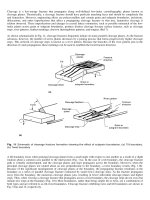
General Contact Analysis. The sliding contact may be considered as two solid bodies, of which one or both move at
uniform speed past a band-shaped heat source (Fig. 1). This source has a heat flux distribution, q, with an average value
of q
av
.

Fig. 1 Schematic showing key parameters that affect heat distribution in an ideal sliding contact model. V
1
and
V
2
, velocities of surface 1 and surface 2, respectively, both velocities being tangential to contact and normal to
contact length; q, heat flux distribution; q
1
and q
2
, portion of heat distribution that penetrates surface 1 and
surface 2, respectively; R
1
and R
2
, radius of curvature of surface 1 and surface 2, respectively; L and w, length
and width, respectively, of heat source
The maximum contact temperature, T
c
, will occur at the surface of either body. It may be simply computed from:

T
c
= T + T

(Eq 7)
where T , the maximum flash temperature of body i (in °C), is superimposed on its respective bulk temperature, T .
Considering that one or both bodies will move relative to the heat source, the maximum flash temperature (in °C) for a
moving surface has been related to the parameters described as:


(Eq 8)
where t represents the time during which any point on the surface is exposed to heat (Ref 5). Variable b denotes a thermal
contact coefficient equal to the square root of the product of the specific heat (c), density ( ), and thermal conductivity (k)
of the material. Coefficient F is dependent on the form of the heat flux distribution, q, over the width of the heat source.
For a square heat source with uniform distribution in which q = q
av
, F is equivalent to 2/(
1/2
) = 1.13, closely
approximating a semielliptical distribution where F = 1.11 (Ref 6). Furthermore, the product · q
av
represents the portion
of heat entering the body where is the heat partition factor. The average total heat flux, q
av
(in W/m
2
), generated by
friction between the two loaded surfaces can be expressed as:
q
av

= · p
av
· V
r


(Eq 9)
where is the coefficient of friction, p
av
is the average pressure according to Hertzian contact theory, and V
r
denotes the
relative sliding velocity between the two surfaces.
Should one of the bodies of Fig. 1 be stationary or moving such that there is sufficient time for the temperature
distribution of a stationary contact to be established, the maximum flash temperature of the body is determined as a
function of its thermal conductivity, k, and the heat flux distribution, q. Table 1 summarizes an assortment of maximum
flash temperature relationships for point and line contacts based on a uniform heat flux distribution, q = q
av
.
Table 1 Selected maximum flash temperature relationships for line and point contacts based on uniform
heat flux distribution

Examples of frictional heating, with both bodies or only one body in motion, are discussed in the sections "Line Contact
Analysis with Two Bodies in Motion" and "Circular Contact Analysis with One Body in Motion" in this article.
Line Contact Analysis with Two Bodies in Motion. Using the model of Fig. 1, the total heat flux developed from
the two moving bodies in line contact must be partitioned (see the section "Heat Partition Factor" in this article). Blok
estimated this by equating the maximum flash temperature of each surface using Eq 8, assuming equivalent bulk
temperatures and a time of contact, t, equal to w/V
i
, where w is the width of the heat source and V

i
is the velocity of body i
(Ref 6). As a result, the portion of heat withdrawn by surface 1 is:


(Eq 10a)
where:


(Eq 10b)
As the two components have equal bulk temperatures T
b
, the contact surface temperature (in °C) of either body can be
simply expressed as:
T
c
= T
f
+ T
b


(Eq 11)
Should both bodies be moving such that the Péclet number of each surface is at least 2, the combination of Eq 8 and 9 for
use in Eq 11 yields T
f
(in °C):


(Eq 12)

where is the coefficient of friction, w is the contact width (in m), L is the contact length (in m), W is the normal contact
load (in N), V
1
and V
2
are velocities (in m/s) of surfaces 1 and 2, tangential to contact and normal to contact length,
respectively, and b
1
and b
2
are thermal contact coefficients of bodies 1 and 2 (W · s
1/2
/m
2
· °C); in which b
i
is:
b
i
= = k
i
/

(Eq 13)
Note that k
i
,
i
, c
i

, and D
i
are the thermal conductivity, density, specific heat per mass, and thermal diffusivity of body i,
respectively. Representative values of common materials are found in Table 2.