Computational Electronics
Semiclassical and Quantum
Device Modeling and Simulation

Dragica Vasileska
Stephen M. Goodnick
Gerhard Klimeck


CRC Press
Taylor & Francis Group
6000 Broken Sound Parkway NW, Suite 300
Boca Raton, FL 33487-2742
© 2010 by Taylor and Francis Group, LLC
CRC Press is an imprint of Taylor & Francis Group, an Informa business
No claim to original U.S. Government works
Printed in the United States of America on acid-free paper
10 9 8 7 6 5 4 3 2 1
International Standard Book Number-13: 978-1-4200-6484-1 (Ebook-PDF)
This book contains information obtained from authentic and highly regarded sources. Reasonable efforts have been made to
publish reliable data and information, but the author and publisher cannot assume responsibility for the validity of all materials
or the consequences of their use. The authors and publishers have attempted to trace the copyright holders of all material reproduced in this publication and apologize to copyright holders if permission to publish in this form has not been obtained. If any
copyright material has not been acknowledged please write and let us know so we may rectify in any future reprint.
Except as permitted under U.S. Copyright Law, no part of this book may be reprinted, reproduced, transmitted, or utilized in any
form by any electronic, mechanical, or other means, now known or hereafter invented, including photocopying, microfilming,
and recording, or in any information storage or retrieval system, without written permission from the publishers.
For permission to photocopy or use material electronically from this work, please access www.copyright.com ( or contact the Copyright Clearance Center, Inc. (CCC), 222 Rosewood Drive, Danvers, MA 01923, 978-750-8400.
CCC is a not-for-profit organization that provides licenses and registration for a variety of users. For organizations that have been
granted a photocopy license by the CCC, a separate system of payment has been arranged.
Trademark Notice: Product or corporate names may be trademarks or registered trademarks, and are used only for identification and explanation without intent to infringe.

Visit the Taylor & Francis Web site at

and the CRC Press Web site at



Contents
Preface.......................................................................................................................................... xiii
Authors ....................................................................................................................................... xvii
1. Introduction to Computational Electronics ...................................................................... 1
1.1 Si-Based Nanoelectronics ............................................................................................ 1
1.1.1 Device Scaling.................................................................................................. 2
1.1.2 Beyond Conventional Silicon ........................................................................ 5
1.1.3 Quantum Transport Effects in Nanoscale Devices .................................... 6
1.2 Heterostructure Devices in III–V or II–VI Technology......................................... 11
1.2.1 Modulation Doping of AlGaAs=GaAs Heterostructures
with In-Plane Transport ............................................................................... 13
1.2.2 Vertical Transport—Resonant Tunneling Devices ................................... 13
1.3 Modeling of Nanoscale Devices............................................................................... 15
1.4 The Content of This Book ......................................................................................... 18
References............................................................................................................................... 20
2. Introductory Concepts......................................................................................................... 23
2.1 Crystal Structure......................................................................................................... 23
2.1.1 Classification of Crystals by Symmetry..................................................... 24
2.1.2 Miller Index.................................................................................................... 26
2.1.3 Reciprocal Space............................................................................................ 29
2.2 Semiconductors........................................................................................................... 32
2.3 Band Structure ............................................................................................................ 36
2.4 Preparation of Semiconductor Materials ................................................................ 40
2.5 Effective Mass ............................................................................................................. 45

2.6 Density of States ......................................................................................................... 54
2.7 Electron Mobility........................................................................................................ 57
2.8 Semiconductor Statistics............................................................................................ 59
2.9 Semiconductor Devices ............................................................................................. 60
2.9.1 Diode............................................................................................................... 62
2.9.2 BJT Transistor ................................................................................................ 65
2.9.3 MOSFET ......................................................................................................... 71
2.9.4 SOI Devices .................................................................................................... 76
2.9.4.1 PD=FD SOI Devices ...................................................................... 76
2.9.5 MESFET .......................................................................................................... 80
2.9.6 HEMTs............................................................................................................ 81
Problems................................................................................................................................. 86
References............................................................................................................................... 94
3. Semiclassical Transport Theory ........................................................................................ 95
3.1 Approximations for the Distribution Function...................................................... 96
3.1.1 Quasi-Fermi Level Concept ......................................................................... 96
3.1.2 Displaced Maxwellian Approximation...................................................... 97
v


vi

Contents

3.2

Boltzmann Transport Equation................................................................................ 98
3.2.1 Scattering Processes .................................................................................... 100
3.3 Relaxation-Time Approximation ........................................................................... 102
3.3.1 Solving the BTE in the Relaxation-Time Approximation ..................... 103

3.4 Rode’s Iterative Method.......................................................................................... 108
3.5 Scattering Mechanisms: Brief Description ............................................................ 111
3.5.1 Phonon Scattering ....................................................................................... 111
3.5.1.1 Acoustic Phonon Scattering ....................................................... 112
3.5.1.2 Nonpolar Optical Phonon Scattering ....................................... 113
3.5.1.3 Polar Optical Phonon Scattering ............................................... 119
3.5.1.4 Piezoelectric Scattering ............................................................... 119
3.5.2 Defect Scattering.......................................................................................... 120
3.5.2.1 Ionized Impurity Scattering ....................................................... 120
3.5.2.2 Neutral Impurity Scattering....................................................... 121
3.5.2.3 Alloy Disorder Scattering........................................................... 121
3.5.3 Electron–Electron Interactions................................................................... 122
3.5.3.1 Electron–Electron Interactions: Binary Collisions................... 122
3.5.3.2 Electron–Plasmon Scattering...................................................... 123
3.5.4 Impact Ionization ........................................................................................ 124
3.6 Implementation of the Rode Method for 6H-SiC Mobility Calculation .......... 125
3.6.1 Relevant Scattering Mechanisms .............................................................. 130
3.6.2 Simulation Results ...................................................................................... 135
3.6.3 Source Code (Provided by Graduate Student Garrick Ng).................. 137
Problems............................................................................................................................... 144
References............................................................................................................................. 147
4. The Drift-Diffusion Equations and Their Numerical Solution ............................... 151
4.1 Drift-Diffusion Model Derivation .......................................................................... 151
4.1.1 Physical Limitations on Numerical Drift-Diffusion Schemes............... 153
4.1.2 Steady-State Solution of the Bipolar Semiconductor Equations .......... 154
4.1.3 Normalization and Scaling ........................................................................ 155
4.1.4 Linearization of Poisson’s Equation ......................................................... 155
4.1.5 Scharfetter–Gummel Discretization of the Continuity Equation ......... 157
4.1.6 Gummel’s Iteration Method ...................................................................... 158
4.1.7 Newton’s Method ....................................................................................... 159

4.1.8 Generation and Recombination ................................................................ 161
4.1.8.1 Carrier Generation Due to Light Absorption.......................... 164
4.1.8.2 Band-to-Band Recombination.................................................... 165
4.1.8.3 Shockley–Read–Hall Generation–Recombination
Mechanism.................................................................................... 165
4.1.8.4 Auger Recombination ................................................................. 166
4.1.8.5 Impact Ionization......................................................................... 167
4.2 Drift-Diffusion Application Examples .................................................................. 168
4.2.1 1D Simulation Example—Modeling of pn-Diode .................................. 168
4.2.2 3D Drift-Diffusion Example: Modeling Threshold Voltage
Fluctuations Due to Discrete Impurities.................................................. 182
Problems............................................................................................................................... 187
References............................................................................................................................. 190


Contents

vii

5. Hydrodynamic Modeling ................................................................................................. 193
5.1 Introduction .............................................................................................................. 193
5.2 Extensions of the Drift-Diffusion Model............................................................... 196
5.3 Stratton’s Approach ................................................................................................. 199
5.4 Hydrodynamic (Balance, Bløtekjær) Equations Model ...................................... 200
5.4.1 Displaced Maxwellian Approximation.................................................... 206
5.4.2 Momentum and Energy Relaxation Rates .............................................. 207
5.4.2.1 Using Drifted-Maxwellian Form for the
Distribution Function.................................................................. 208
5.4.2.2 Using Bulk Monte Carlo Simulations....................................... 209
5.4.3 Simplifications That Lead to the Drift-Diffusion Model ....................... 209

5.4.4 Discretization and Numerical Solution Schemes
for the Hydrodynamic Equations............................................................. 210
5.4.4.1 von Neumann Stability Analysis .............................................. 212
5.4.4.2 Lax Method .................................................................................. 212
5.4.4.3 Other Varieties of Error .............................................................. 214
5.4.4.4 Second-Order Accuracy in Time ............................................... 215
5.4.4.5 Fluid Dynamics with Shocks ..................................................... 218
5.5 The Need for Commercial Semiconductor Device Modeling Tools ................. 219
5.5.1 Key Elements of Physical Device Simulation ......................................... 220
5.5.2 Historical Development of the Physical Device Modeling ................... 220
5.6 State-of-the-Art Commercial Packages ................................................................. 222
5.6.1 Silvaco ATLAS............................................................................................. 222
5.6.2 Synopsys Software ...................................................................................... 225
5.7 The Advantages and Disadvantages of Hydrodynamic Models:
Simulations of Different Generation FD SOI Devices......................................... 227
Problems............................................................................................................................... 234
References............................................................................................................................. 239
6. Particle-Based Device Simulation Methods ................................................................. 241
6.1 Direct Solution of Boltzmann Transport Equation:
Monte Carlo Method ............................................................................................... 242
6.1.1 Free-Flight Generation................................................................................ 243
6.1.2 Final State after Scattering ......................................................................... 244
6.1.3 Ensemble Monte Carlo Simulation........................................................... 245
6.1.4 Scattering Processes .................................................................................... 246
6.1.5 Bulk Monte Carlo Code for GaAs ............................................................ 248
6.2 Multi-Carrier Effects ................................................................................................ 286
6.2.1 Pauli Exclusion Principle ........................................................................... 288
6.2.2 Carrier–Carrier Interactions....................................................................... 288
6.2.3 Band-to-Band Impact Ionization............................................................... 290
6.2.4 Full-Band Particle-Based Simulation........................................................ 291

6.3 Device Simulations................................................................................................... 292
6.3.1 Calculation of the Current ......................................................................... 294
6.3.2 Ohmic Contacts ........................................................................................... 297
6.3.3 Time-Step...................................................................................................... 298
6.3.4 Particle-Mesh Coupling.............................................................................. 299
6.3.5 Source Code for Modeling FD SOI Devices............................................ 301


viii

Contents

6.4

Coulomb Force Treatment within a Particle-Based
Device Simulation Scheme...................................................................................... 306
6.4.1 Particle–Particle–Particle–Mesh Approach.............................................. 311
6.4.2 Corrected Coulomb Scheme ...................................................................... 313
6.4.3 Fast Multipole Method............................................................................... 315
6.4.3.1 Multipole Moment....................................................................... 316
6.4.3.2 Speedup of the FMM Algorithm............................................... 317
6.5 Representative Simulation Results of Multiparticle
and Discrete Impurity Effects................................................................................. 318
6.5.1 The Role of Short-Range e–e and e–i Interactions .................................. 319
6.5.2 Fluctuations in the On-State Currents ..................................................... 322
6.5.3 Current Issues in Novel Devices—Unintentional Dopants .................. 324
Problems............................................................................................................................... 329
References............................................................................................................................. 332
7. Modeling Thermal Effects in Nano-Devices................................................................ 335
7.1 Some General Aspects of Heat Conduction......................................................... 337

7.2 Classical Heat Conduction in Solids ..................................................................... 342
7.3 Form of the Heat Source Term............................................................................... 343
7.4 Modeling Heating Effects with Commercial Simulation Packages .................. 345
7.4.1 Thermal3D Package from Silvaco............................................................. 345
7.4.2 GIGA3D—Non-Isothermal Device Simulator ........................................ 347
7.5 The ASU Particle-Based Approach to Lattice Heating
in Nanoscale Devices ............................................................................................... 349
7.5.1 Electrothermal Particle–Based Device Simulator Description.............. 352
7.5.2 Thermal Degradation with Device Scaling ............................................. 359
7.6 Open Problems ......................................................................................................... 363
Problems............................................................................................................................... 364
References............................................................................................................................. 364
8. Quantum Corrections to Semiclassical Approaches ................................................... 367
8.1 One-Dimensional Quantum-Mechanical Space Quantization........................... 369
8.1.1 Description of SCHRED............................................................................. 370
8.1.1.1 Capacitance Degradation ........................................................... 379
8.1.1.2 Threshold Voltage ....................................................................... 380
8.1.2 Modification of the Effective Mass Schrödinger Equation
for Heterostructures.................................................................................... 381
8.2 Quantum Corrections to Drift-Diffusion and Hydrodynamic Simulators ...... 383
8.2.1 Quantum Correction Approaches ............................................................ 383
8.2.2 Quantum Moment Methods...................................................................... 384
8.3 The Effective Potential Approach in Conjunction
with Particle-Based Simulations............................................................................. 387
8.3.1 Effective Potential Approach..................................................................... 387
8.3.2 Effective Potential from the Wigner–Boltzmann Equation................... 388
8.4 Description of Gate Current Models Used in Device Simulations ................... 394
8.4.1 Oxide Charging and Tunneling ................................................................ 395
8.4.2 Hot Carrier Injection................................................................................... 397
8.4.3 Gate Leakage Calculation in Conjunction with Particle-Based

Device Simulators ....................................................................................... 399


Contents

ix

Monte Carlo—k Á p—1D Schrödinger Solver for Modeling Transport
in p-Channel Strained SiGe Devices ...................................................................... 405
8.5.1 Transport in SiGe p-Channel MOSFETs .................................................. 406
8.5.2 The Six-Band k Á p Model Applied to Valence Band Structure
of Si and Ge ................................................................................................. 411
8.5.2.1 Valence Band Structure in Si Inversion
Layers—2D Dispersion Problem ............................................... 413
8.5.2.2 Valence Band Structure in Strained Layer Heterostructure
MOSFET Inversion Layers ......................................................... 416
8.5.2.3 Valence Band Structure in Inversion Layers—2D
Contour Problem ......................................................................... 420
8.5.2.4 Description of the Self-Consistent Scheme .............................. 422
8.5.2.5 Density of States .......................................................................... 424
8.5.3 Monte Carlo Procedure and Simulation Results .................................... 425
8.5.3.1 Carrier Scattering Rates .............................................................. 425
8.5.3.2 2D $ 3D Transitions .................................................................. 429
8.5.5.3 Simulation Results....................................................................... 429
Problems............................................................................................................................... 436
References............................................................................................................................. 438

8.5

9. Quantum Transport in Semiconductor Systems ......................................................... 445

9.1 Tunneling................................................................................................................... 446
9.2 General Notation ...................................................................................................... 448
9.2.1 Stationary States for a Free Particle.......................................................... 453
9.2.2 Potential Step ............................................................................................... 453
9.2.3 Tunneling through a Single Barrier.......................................................... 458
9.3 Transfer Matrix Approach ...................................................................................... 461
9.3.1 Basic Description of the Method............................................................... 461
9.3.2 Piecewise Constant Potential Barrier Tool .............................................. 462
9.3.2.1 Example for Quantum Mechanical
Reflections..................................................................................... 463
9.3.2.2 Is There Source-to-Drain Tunneling in Nanoscale
MOSFETs? .................................................................................... 464
9.3.2.3 Quasi-Bound States Formation in a Double-Barrier
Structure........................................................................................ 465
9.3.2.4 Formation of Energy Bands ....................................................... 468
9.3.2.5 More Complex PCPBT Capabilities That Utilize
a Tight-Binding Approach ......................................................... 469
9.3.3 Limitations of Transfer Matrix Approach
and Its Alternatives..................................................................................... 470
9.4 Landauer Formula and Usuki Method ................................................................. 471
9.4.1 Landauer–Büttiker Formalism .................................................................. 472
9.4.2 Usuki Iterative Procedure .......................................................................... 473
9.4.2.1 Spin Transport and Spin Filter .................................................. 475
9.4.2.2 Theoretical Modeling of Spin Filters ........................................ 477
9.4.2.3 Simulation Results for Spin Filter ............................................. 479
Problems............................................................................................................................... 484
References............................................................................................................................. 489


x


Contents

10. Far-From-Equilibrium Quantum Transport.................................................................. 493
10.1 Mixed States and Distribution Function............................................................... 493
10.2 Irreversible Processes and MASTER Equations................................................... 495
10.3 The Wigner Distribution Function......................................................................... 496
10.4 Green’s Functions..................................................................................................... 498
10.4.1 Mathematical Physics Formulation of the Green’s
Function Method ......................................................................................... 499
10.4.1.1 Schrodinger, Heisenberg, and Interaction Representation.... 499
10.4.1.2 Wick’s Theorem and Perturbation Series Generation............ 501
10.4.1.3 Dyson Equation for the Retarded Green’s Function.............. 503
10.4.1.4 Equilibrium Properties of a Semiconductor—GW
Approximation............................................................................. 505
10.5 Nonequilibrium Keldysh Green’s Functions........................................................ 506
10.5.1 Need for Approximations to the NEGF Formalism—Application
Targets .......................................................................................................... 512
10.6 Low Field Transport in Strained-Si Inversion Layers......................................... 513
10.6.1 Theoretical Model ....................................................................................... 513
10.6.2 Calculation of the Broadening of the States
and Conductivity=Mobility ....................................................................... 517
10.6.3 Electron Mobility Results—Low Doped Samples .................................. 520
10.6.4 Electron Mobility Results—Highly Doped Samples.............................. 523
10.7 NEGF in a Quasi-1D Formulation ......................................................................... 526
10.7.1 Tight-Binding Hamiltonian ....................................................................... 526
10.7.2 Recursive Green’s Functions Method for the Retarded
Green Function ............................................................................................ 527
10.7.3 Recursive Green’s Functions Method for the Less Than
Green Function ............................................................................................ 529

10.7.4 NEGF with Incoherent Scattering............................................................. 531
10.7.5 Open Boundary Condition Formulation ................................................. 531
10.7.6 1D Effective Mass Hamiltonian and Boundary Conditions ................. 533
10.8 Quantum Transport in 1D—Resonant Tunneling Diodes ................................. 534
10.8.1 RTDs with Linear Potential Drops ........................................................... 535
10.8.2 RTDs with Realistic Doping Profiles........................................................ 542
10.8.3 Resonant Tunneling Diodes with Relaxation in the Reservoirs........... 547
10.8.4 RTDs with Quantum Charge Self-Consistency (Hartree Model) ........ 551
10.8.5 Asymmetric RTDs with Charge Accumulation and Depletion ........... 555
10.8.6 Resonant Tunneling Diode Simulations with Incoherent
Scattering ...................................................................................................... 561
10.8.7 RTD Simulations at Room Temperature with Full
Bandstructure............................................................................................... 565
10.9 Coherent High-Field Transport in 2D and 3D..................................................... 568
10.9.1 Full Atomistic Quantum Transport in OMEN ....................................... 568
10.9.2 2D Effective Mass Hamiltonian and Boundary Conditions ................. 569
10.9.3 High-Field Transport—CBR Algorithm (Denis Mamaluy) .................. 570
10.9.3.1 Bound States Treatment ............................................................. 572
10.9.3.2 CBR Energy Discretization......................................................... 574
10.9.3.3 CBR Self-Consistent Solution..................................................... 574
10.9.3.4 Device Hamiltonian, Algorithm, and Some
Numerical Details........................................................................ 575


Contents

xi

10.9.3.5 CBR Simulation Example—2D Results .................................... 577
10.9.3.6 CBR Simulation Example—3D Results .................................... 580

Problems............................................................................................................................... 592
References............................................................................................................................. 593
11. Conclusions ......................................................................................................................... 599
References............................................................................................................................. 601
Appendix A: Electronic Band Structure Calculation ......................................................... 605
A.1 Spin-Orbit Coupling ................................................................................................ 606
A.2 Rashba and Dresselhaus Spin Splitting ................................................................ 608
A.2.1 Empirical Pseudopotential Method.......................................................... 608
A.2.1.1 Description of the Empirical Pseudopotential Method ......... 611
A.2.1.2 Implementation of the Empirical Pseudopotential
Method for Si and Ge ................................................................. 613
A.2.1.3 Empirical Pseudopotential Method for GaN........................... 615
A.2.2 The Tight-Binding Method ........................................................................ 616
A.2.3 The k Á p Method.......................................................................................... 619
A.2.3.1 k Á p General Description ............................................................ 619
A.2.3.2 k Á p Theory Near the G Point and for Bulk Materials ........... 620
A.2.3.3 Kane’s Theory .............................................................................. 622
A.2.3.4 Coupling with Distant Bands .................................................... 626
A.2.3.5 The Luttinger–Kohn Hamiltonian............................................. 627
A.2.4 Carrier Dynamics ........................................................................................ 630
References............................................................................................................................. 630
Appendix B: Poisson Equation Solvers ................................................................................ 633
B.1 Maxwell’s Equations................................................................................................ 633
B.1.1 Case without Magnetic or Dielectric Materials ...................................... 635
B.1.2 Case of Linear Materials ............................................................................ 635
B.1.3 General Case ................................................................................................ 635
B.2 Gauge Transformations ........................................................................................... 636
B.2.1 Lorenz Gauge .............................................................................................. 637
B.2.2 Coulomb Gauge .......................................................................................... 637
B.3 General Guidelines for Solving Partial Differential Equations.......................... 638

B.4 Finite Difference Discretization of the Poisson Equation................................... 639
B.4.1 Finite Difference Discretization................................................................. 640
B.4.2 Linearization of the Poisson Equation ..................................................... 642
B.4.3 Final Expressions......................................................................................... 642
B.5 Numerical Solution Techniques for 2D=3D Poisson Equation.......................... 644
B.5.1 Direct Methods ............................................................................................ 645
B.5.1.1 Gauss Elimination Method ........................................................ 645
B.5.1.2 The LU Decomposition Method................................................ 646
B.5.2 Iterative Methods ........................................................................................ 648
B.5.2.1 The Gauss–Seidel Method.......................................................... 648
B.5.2.2 The Successive Over-Relaxation Method................................. 649
B.5.2.3 Other Iterative Methods ............................................................. 650
References............................................................................................................................. 670


xii

Contents

Appendix C: Computational Electromagnetics ................................................................... 673
C.1 Introduction .............................................................................................................. 673
C.2 Maxwell’s Equations................................................................................................ 673
C.2.1 Implicit Enforcement of Gauss’ Law........................................................ 674
C.3 Finite-Difference Time Domain Method ............................................................... 676
C.3.1 Accuracy and Numerical Dispersion ....................................................... 680
C.3.2 Stability ......................................................................................................... 681
C.4 Absorbing Boundary Conditions........................................................................... 681
C.4.1 Overview ...................................................................................................... 681
C.4.2 Perfectly Matched Layer ............................................................................ 682
C.4.3 Convolutional Perfectly Matched Layer.................................................. 684

C.4.3.1 Background .................................................................................. 684
C.4.3.2 Stretched-Coordinate Formulation
of Maxwell’s Equations .............................................................. 684
C.4.3.3 General Formulation of the CPML-FDTD
Algorithm ..................................................................................... 686
C.5 Alternate-Direction Implicit-FDTD Method......................................................... 692
C.5.1 Background .................................................................................................. 692
C.5.2 General Formulation of the ADI-FDTD Algorithm ............................... 693
C.5.3 Conventional Split-Field PML Formulation
of the ADI-FDTD Algorithm ..................................................................... 696
C.5.4 CPML Formulation of the ADI-FDTD Algorithm ................................. 697
C.6 Validation of Full-Wave FDTD Solvers ................................................................ 699
C.6.1 Introduction ................................................................................................. 699
C.6.2 Modeling Excitation Sources ..................................................................... 700
C.6.2.1 Hard Sources ................................................................................ 700
C.6.2.2 Soft Sources .................................................................................. 701
C.6.3 Analysis of 3D Planar Microstrip Circuits .............................................. 702
C.6.3.1 Rectangular Patch Antenna ....................................................... 702
C.6.3.2 Low-Pass Filter............................................................................. 705
C.6.4 Photonic Crystals ........................................................................................ 708
C.6.4.1 Simulation of Photonic Crystal Waveguides........................... 709
C.6.5 Summary ...................................................................................................... 713
References............................................................................................................................. 714
Appendix D: Stationary and Time-Dependent Perturbation Theory............................. 717
D.1 Stationary Perturbation Theory.............................................................................. 717
D.1.1 Examples of Stationary Perturbation Theory.......................................... 725
D.1.1.1 The Stark Effect in a Potential Well .......................................... 725
D.1.1.2 Harmonic Oscillator with Linear Perturbation ....................... 727
D.2 Time-Dependent Perturbation Theory .................................................................. 729
D.2.1 Example That Shows the Conditions for the Validity

of Fermi’s Golden Rule .............................................................................. 736
D.2.2 Application of Fermi’s Golden Rule to Elastic Scattering
of Electrons................................................................................................... 738
References............................................................................................................................. 746
Index ............................................................................................................................................ 747


Preface
The purpose of this book is to introduce interested scientists from academia and industry
to advanced simulation methods needed for modeling state-of-the-art nanoscale devices.
The book also serves as a textbook for two graduate-level modeling classes: one devoted to
semiclassical transport modeling and the second dedicated completely to quantum transport modeling.
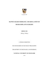
This book provides an overview of the basic techniques used in the field of computational electronics related to device simulation. The multiple scale transport in semiconductors is summarized in Figure 1 in terms of the transport regimes, relative importance of
the scattering mechanisms, length scales such as critical device lengths L, electron wavelength l, electron–electron scattering length le-e, electron–phonon scattering length le-ph, and
possible applications.
We believe that this book has been written at the right time, namely, during an era when
the transistor is reaching its limits, and when new device designs and paradigms of device
operation are being explored.
In the first half of the book, we cover semiclassical methods for semiconductor device
modeling; we begin with the simple drift-diffusion model and then provide a description
of the hydrodynamic and energy balance transport. We conclude the semiclassical transport modeling with a comprehensive discussion on particle-based device simulation
methods. In addition to focusing on the theory, equal emphasis is placed on the numerical
solution approach used for the particular methods that are described. For example, when
talking about the drift-diffusion model and its derivation from the Boltzmann transport
equation, we also discuss the Sharfetter–Gummel discretization scheme that relaxes some

L << le−ph
L<λ

L < le−e


L ~ le−ph

L >> le−ph

L >> le−e

Transport regime

Quantum

Ballistic

Fluid

Scattering

Rare

Rare

e–e (Many), e–ph (Few)

Fluid

Diffusive
Many

Model:
Drift-diffusion

Hydrodynamic

Quantum hydrodynamic

Monte Carlo

Schrödinger equation
Green’s function
Applications

Nanowires,
superlattices

Ballistic
transistor

Present time
ICs

Present time
ICs

Older ICs

FIGURE 1
Relationship between various transport regimes and significant length scales.

xiii



xiv

Preface

constraints on the mesh size and leads to improved convergence of either the Gummel or
the Newton method used for solving the coupled set of Poisson and current continuity
equations. This is what distinguishes this book from other texts in the literature that are
focused only on the theoretical aspect of semiconductor transport. Implementation is
necessary for computer device designs, and this is exactly what this book provides to the
readers: a comprehensive overview of methods for analyzing transport in semiconductor
devices, beginning from the simplest semiclassical approaches and ending with a description of the most complex, fully quantum mechanical methods for quantum transport
analysis of novel state-of-the-art devices.
The second half of the book begins with a discussion highlighting the need for quantum
transport, the description of various quantum effects appearing in current and future
devices that are either being mass-produced or fabricated as a proof of concept. In this
context, we introduce the concept of effective potential used to approximately include
quantum mechanical space-quantization effects within the semiclassical particle-based
device simulation scheme. Moving into the next chapter, where we talk about open
quantum systems, we introduce tunneling as a purely quantum mechanical concept and
we discuss ways of calculating the tunneling coefficient for arbitrary piecewise constants
and piecewise linear potential barriers. The Landauer–Buttiker formula for the calculation
of the conductance is introduced next as a way of studying quantum mechanical systems in
a linear-response (near-equilibrium) regime of operation. The next chapter is dedicated to
the far-from-equilibrium quantum transport. Several methods, with different levels of
complexities and accuracies, are explained in detail when solving the far-from-equilibrium
quantum transport problem, including the Wigner function and Green’s function methods.
Since the emphasis in this book is on Green’s function method for solving the quantum
transport problem, we describe in detail the recursive Green’s function method and its
variant, the Usuki method. Then we describe the contact block reduction method as the
most efficient and most complete way of solving the quantum transport problem since this

method allows one to simultaneously calculate source–drain current and gate leakage,
which is not the case, for example, with the Usuki and the recursive Green’s function
techniques that are in fact quasi-1D in nature for transport through a device. We summarize this book with some open questions related to quantum transport that were not
previously covered here.
Many people have contributed either directly or indirectly to make this book a reality.
The authors would first like to thank Professor David K. Ferry for the many valuable
discussions that they have had with him in the course of the preparation of the material for
this book and before. Many thanks go to Professor Dieter Schroder who has been an
inspiration to Professor Dragica Vasileska not only at the professional level, but on a
personal level as well. Professor Christian Ringhofer has been a very valuable resource
when developing most of the codes that have been implemented at Arizona State University and for the generalization of the effective potential scheme. Other people who have
had a significant impact on the research presented in this book include Dr. Denis Mamaluy;
Dr. Jason Ayobi-Moak (contributed Appendix C—Computational Electromagnetics);
Professors Mark Lundstrom and Supriyo Datta from Purdue University, West Lafayette,
Indiana; and many others from the Center for Solid State Electronics Research at Arizona
State University, Tempe. Dr. Jean Michel Sellier, Dr. Mathieu Luisier, Samarth Agarwal,
and Abhijeet Paul helped at Purdue to shape some of the nanoHUB.org tools that have
been used in this book.
Professor Vasileska wants to take this opportunity to thank her parents, Antigona and
Zdravko Vasileski, for supporting her and being with her always, most importantly in


Preface

xv

difficult times. She would also like to thank her niece, Emili Vasileska, and her nephew,
Zdravko Vasileski, for all their love. Professor Goodnick thanks the invaluable support and
patience of Sara for many late nights involved in the writing and proofing of this text.
Professor Gerhard Klimeck thanks his family, Ginny, George, and Gabrielle, for the love,

support, patience, and acceptance during the times of intense work.



Authors
Dragica Vasileska received her BSEE (diploma) and MSEE from the University Sts. Cyril
and Methodius, Skopje, Republic of Macedonia, in 1985 and 1992, respectively, and her
PhD from Arizona State University, Tempe, in 1995. From 1995 to 1997, she held a faculty
research associate position within the Center of Solid State Electronics Research at Arizona
State University. In the fall of 1997, she joined the faculty of electrical engineering at
Arizona State University. In 2002, she was promoted to associate professor and in 2007
to full professor. Her research interests include semiconductor device physics and semiconductor device modeling, with strong emphasis on quantum transport and Monte Carlo
particle–based simulations. She is a senior member of the Institute of Electrical and
Electronics Engineering (IEEE) and American Physical Society (APS). Dr. Vasileska has
published more than 140 journal publications, over 80 conference proceedings refereed
papers, has given numerous invited talks, and is a coauthor of a book on computational
electronics with Professor S.M. Goodnick. She has many awards including the best student
award from the School of Electrical Engineering in Skopje since its existence (1985, 1990).
She is also a recipient of the 1998 NSF CAREER Award. Her students won the best
paper and the best poster award at the Low Dimensional Structures and Devices (LDSD)
conference in Cancun, 2004.
Stephen M. Goodnick received his BS in engineering science from Trinity University, San
Antonio, Texas, in 1977, and his MS and PhD in electrical engineering from Colorado State
University, Fort Collins, in 1979 and 1983, respectively.
He was an Alexander von Humboldt Fellow with the Technical University of Munich,
Germany, and the University of Modena, Italy, in 1985 and 1986, respectively. He was a
faculty member from 1986 to 1997 with the Department of Electrical and Computer
Engineering at Oregon State University, Corvallis, and served as chair and professor of
electrical engineering with Arizona State University, Tempe, from 1996 to 2005. He served
as deputy dean for the Ira A. Fulton School of Engineering, Tempe, Arizona, during 2005–

2006, and as associate vice president for research for Arizona State University from 2006 to
2008. He is currently the director of the Arizona Initiative for Renewable Energy and the
Arizona Institute for Nanoelectronics, Tempe, Arizona. His main research interests are in
transport in semiconductor devices, computational electronics, quantum and nanostructured devices and device technology, and high-frequency and optical devices. Some of his
main contributions include the analysis of surface roughness at the Si=SiO2 interface,
Monte Carlo simulation of ultrafast carrier relaxation in quantum confined systems, global
modeling of high frequency devices, full-band simulation of semiconductor devices, transport in nanostructures, and fabrication and characterization of nanoscale semiconductor
devices. He has published over 185 refereed journal articles, books, and book chapters and
is a fellow of the IEEE (2004).
Gerhard Klimeck is the director of the Network for Computational Nanotechnology
(NCN), West Lafayette, Indiana, and a professor of electrical and computer engineering
at Purdue University, West Lafayette, Indiana. He guides the developments and strategies
of nanoHUB.org, which served over 89,000 users worldwide with online simulation,
tutorials, and seminars in the year 2008. He served as NCN technical director from 2003
xvii


xviii

Authors

to May 2009. He was the technical group supervisor of the High Performance Computing
Group and a principal scientist at the NASA Jet Propulsion Laboratory (JPL), Pasadena,
California, from 1998 to 2003. Prior to this, he was a member of the technical staff at the
Central Research Lab of Texas Instruments, Dallas, where he served as a manager and
principal architect of the Nanoelectronic Modeling (NEMO 1D) program. NEMO 1D was
the first quantitative simulation tool for resonant tunneling diodes and 1D heterostructures. At JPL and Purdue, Gerhard developed the Nanoelectronic Modeling tool (NEMO 3D)
for multimillion atom electronic structure simulations. NEMO 3D has been used to quantitatively model optical properties of self-assembled quantum dots, disordered Si=SiGe
systems, and single impurities in silicon. At Purdue, his group is developing a new simulation
engine that combines the NEMO 1D and NEMO 3D capabilities into a new code entitled

OMEN. OMEN has demonstrated almost perfect scaling to over 200,000 parallel cores.
Professor Klimeck’s research interest is in the modeling of nanoelectronic devices,
parallel computing, and genetic algorithms. He received his PhD (on quantum transport) in
1994 from Purdue University and his German electrical engineering degree in 1990 from
Ruhr-University Bochum, Germany. Dr. Klimeck’s work is documented in over 130 peerreviewed journals, 120 proceedings publications, and over 120 invited and 270 contributed
conference presentations, and has been cited over 2500 times. He is a senior member of the
IEEE and a member of APS, Eta Kappa Nu (HKN) and Tau Beta Pi (TBP).


1
Introduction to Computational Electronics

1.1 Si-Based Nanoelectronics
The semiconductor device–based electronics industry is the largest industry in the world
with global sales of over $1 trillion since 1998. If current trends continue, the sales volume
of the electronics industry will reach $3 trillion and will constitute about 10% of the gross
world product (GWP) by 2010 [1]. The revolution in the semiconductor industry, a subset
of the electronics industry, began in 1947 with the fabrication of bipolar devices on slabs of
polycrystalline germanium (Ge) [2], as shown in the summary of the major milestones in
the early history of semiconductors in Figure 1.1.
Single-crystal materials were later introduced, making possible the fabrication of epitaxially grown junction transistors. The migration to silicon (Si)-based devices was initially
hindered by the stability of the Si=SiO2 materials system, necessitating a new generation of
crystal pullers with improved environmental controls to prevent SiO2 formation. Later, the
stability and low interface-state density of the Si=SiO2 interface provided passivation of
surfaces and eventually the transition from bipolar devices to field-effect devices in 1960.
By 1968, both complementary metal–oxide–semiconductor devices (CMOS) and polysilicon gate technology, which allowed self-alignment of the gate to the source=drain of the
device, had been developed. These innovations permitted a significant reduction in
power dissipation and a reduction of the device overlap capacitance, improving frequency
performance and resulting in the essential components of the modern CMOS device.
Advances in compound semiconductor heterostructure devices from heterostructure bipolar transistors [3] to lasers* have paved the way for novel heterostructure devices including

those in silicon. The unique properties of the variety of semiconductor materials have
enabled the development of a wide variety of ingenious devices that have literally changed
our world. To date, there are about 60 major devices with over 100 device variations
related to them.
The metal oxide semiconductor field effect transistor (MOSFET) and related integrated
circuits now constitute about 90% of the semiconductor device market. Combining silicon
with the elegance of the field-effect transistor (FET) structure has allowed making devices
smaller, faster, and cheaper. Nowadays, the primary factor driving the continuous
improvement in device performance is the semiconductor industry’s relentless effort to
reduce the cost per function on a chip. This cost reduction is realized by fabricating more
devices on a chip while either reducing manufacturing costs or holding them constant.

* In 1954, Charles Townes and Arthur Schawlow invented the maser. Theodore Maiman invented the ruby laser
considered to be the first successful optical or light laser. Many historians claim that Theodore Maiman invented
the first optical laser, however, there is some controversy that Gordon Gould was the first.

1


2

Computational Electronics

-

Bipolar transistor
Monocrystal germanium
First good BJT
Monocrystal silicon
Oxide mask,

commercial silicon BJT
Transistor with diffused
base
Integrated circuit
Planar transistor
Planar integrated circuit
Epitaxial transistor
MOSFET
Schottky diode
Commercial integrated
circuit (RTL)

1947
1950
1951
1951
1954
1955
1958
1959
1959
1960
1960
1960
1961

-

DTL technology
TTL technology

ECL technology
MOS integrated circuit
CMOS
Linear integrated circuit
MSI circuits
MOS memories
LSI circuits
MOS processor
Microprocessor
I2L
VLSI circuits
Computers using
VLSI technology
- ...

1962
1962
1962
1962
1963
1964
1966
1968
1969
1970
1971
1972
1975
1977


FIGURE 1.1
Some historical dates.

There are three primary methods for reducing the cost per function. The first is transistor
scaling, which involves reducing the transistor size in accordance with some goal, e.g.,
keeping the electric field constant from one generation to the next. Smaller transistors enable
more of them to fit within a given area, while allowing them to operate faster than previous
generations. The second method is circuit cleverness, which is associated with the physical
layout of the transistors with respect to each other. If more functionality can be realized with
fewer transistors, then the computational capability per die is increased. The third method is
to make the die larger. More devices can be fabricated on a larger die. Meanwhile, the
semiconductor industry is constantly looking for technological breakthroughs to decrease
the manufacturing cost. All of these efforts serve to reduce the cost per function on a chip.
1.1.1 Device Scaling
Device engineers are most concerned with methods of size down scaling. The semiconductor industry has been so successful in providing continued system performance
improvement year after year that the Semiconductor Industry Association (SIA) has been
publishing roadmaps for semiconductor technology since 1992. These roadmaps represent
a consensus outlook of industry trends using history as a guide. Recent roadmaps [4]
incorporate participation from the global semiconductor industry, including the United
States, Europe, Japan, Korea, and Taiwan. They basically affirm the desire of the industry
to continue with Moore’s law [5], which is often stated as a doubling of transistor
performance and a quadrupling of the number of devices on a chip every 3 years. The
phenomenal progress signified by Moore’s law has been achieved through the scaling of
the MOSFET from larger to smaller physical dimensions. Scaling of CMOS technology has
progressed relentlessly from a line width of 1 mm to the current 32 nm line width at the
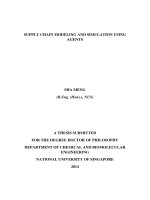
time of publication of this book. Two key features characterize this era. First, slavish
devotion to scaling by constant improvements in lithography (see Figure 1.2, top panel),
as described by Dennard et al. [6]. The second key feature is a minimal rate of introduction
of substantially new materials and structures. Substantial effort is required to introduce
new materials, and great effort is required to ensure that both manufacturability

and reliable integration be attained. Significant efforts currently under way include


3

Introduction to Computational Electronics

1

1000
Wave length
248 nm

OPC

0.1

100

Phase shift
immersion

nm

Microns

193 nm

32 nm
EUV

22 nm
Feature size
15 nm 13.5 nm
0.01
1980

1990

2000
Lithography

2010

10
2020

10
CPU transistor count
2× every 2 years

109

1
Microns

107

0.1

0.01

1970

Feature size
0.7× every 2 years

65 nm
45 nm
32 nm

105

103
2000
2010
2020
1980
1990
Transistor dimensions scale to improve performance,
reduce power and reduce cost per transistor
Scaling trends

FIGURE 1.2
Top panel: Needed improvements in lithography. Bottom panel: Transistor scaling as seen by Intel. (Courtesy of
K. David, Intel Corp. www.intel.com)

identification for a replacement of silicon dioxide as the gate dielectric for MOSFETs and,
recently, announcements regarding the introduction of silicon–germanium in CMOS technology give further evidence of the forces for change.
Regarding conventional silicon MOSFETs, the device size is scaled in all dimensions (see
Figure 1.2, bottom panel) resulting in smaller oxide thickness, junction depth, channel
length, channel width, and isolation spacing. The SIA forecasts that this exponential scaling

of silicon (or silicon-compatible) FETs and integrated circuits will continue at least until the
year 2015, when devices with 10 nm features should become commercially available.
Groups from both Toshiba and Lucent Bell Labs have fabricated n-channel MOSFETs
with effective gate lengths below 25 nm [7,8] and thus demonstrated that these feature
sizes are feasible. An ultrasmall MOSFET with a channel length of 15 nm has been
demonstrated in 2001 [9]. Conventional silicon MOS transistors with a physical gate length


4

Computational Electronics

of 10 nm have been demonstrated by Intel Corporation [10]. These devices can serve as the
basis for the most advanced integrated circuit chips containing over 1 trillion (>1012)
devices. Intel has begun manufacturing some chips based on this new process with gigabit
Ethernet, optical networking, and wireless ICs among the applications. Device miniaturization also reduces the energy used for each switching operation. The energy dissipated
per logic gate has decreased by over 1 million times since 1959. But since more devices are
packed into the same area, operating at increasing frequencies, the actual total energy
consumption per chip has slowly increased over the years to over 100 W per CPU, resulting
in intense heat generation on a very small Si chip.
It is important to point out that the exponential growth in integrated circuit complexity,
which has seen a 100-million-fold increase in transistor count per chip over the past
40 years, is finally facing its limits. Limits projected in the past have seemingly vanished
before the concerted efforts of researchers and technologists, yet this time the limits seem
more real and are already forcing new strategies on the design of future devices. Critical
dimensions, such as transistor gate length and oxide thickness, are reaching physical
lengths of a countable number of atoms. Maintaining dimensional integrity at the limits
of scaling is a challenge. Considering the manufacturing issues, photolithography becomes
difficult as the feature sizes approach the wavelength of ultraviolet light. In addition, it is
difficult to control the oxide thickness when the oxide is made up of just a few atomic

monolayers. Processes will be required that approach atomic-layer precision. Just being
able to model future processes to predict geometries and doping concentrations of future
devices is a challenge that has not been met. The existing empirical techniques will have to
be aided by increasingly sophisticated ab initio calculations in order to reduce the experimental parameter space to manageable proportions.
In addition to the processing issues, there are also some fundamental device issues.
Shrinking the conventional MOSFET beyond the 50 nm technology node requires innovations to circumvent barriers due to the fundamental physics that constrain a conventional
MOSFET. The limits most often cited [11] include: (1) quantum-mechanical tunneling of
carriers through the thin gate oxide; (2) quantum-mechanical tunneling of carriers from
source to drain and from drain to the body of the MOSFET; (3) control of the density and
location of dopant atoms in the MOSFET channel and source=drain region to provide a
high on-off current ratio; (4) control of threshold voltage over the die is another major
scaling challenge; (5) voltage-related effects such as subthreshold swing, built-in voltage,
and minimum logic voltage swing; (6) short-channel effects (SCEs), such as drain-induced
barrier lowering (DIBL) that degrade the device performance; (7) hot carriers that degrade
device reliability; and (8) other application-dependent power-dissipation limits. For
analog=RF applications, additional challenges include sustaining linearity, low noise
figure, power-added efficiency, and transistor matching.
The quickening pace of MOSFET technology scaling is accelerating the introduction of
many new technologies to extend CMOS into nanoscale MOSFET structures heretofore not
thought possible, as shown in Figure 1.3. Optimism is emerging that these new technologies may extend MOSFETs to the 22 nm node (9 nm physical gate length) by 2016 if not by
the end of this decade. These new devices will likely feature several new materials cleverly
incorporated into new nonbulk MOSFET structures. Intrinsic device speeds may be more
than 1 THz and integration densities will exceed 1 billion transistors=cm2. Excessive power
consumption, however, will demand the judicious use of these high-performance devices
only in those critical paths requiring their superior performance. Two or perhaps three
other lower performance, more power-efficient MOSFETs will likely be used to perform
less performance-critical functions on the chip to manage the total power consumption.


5


Introduction to Computational Electronics

65 nm
2005

45 nm
2007

22 nm
2011

32 nm
2009

Manufacturing

16 nm
2013

Development

Research
Nanowire

III-V

3-D

11 nm

2015

S D
S
Computational
lithography G Metal
h-k
Hig

5 nm
Optical
interconnect

Ge
Dense SRAM

CU
barrier

Carbon
nanotube FET

Novel technology options are being explored in the
pipeline to ensure the continuance of Moore’s law

Innovation-enabled technology pipeline
FIGURE 1.3
A view from Intel on future technology nodes. (Courtesy of R. Chau, Intel Corp.)

1.1.2 Beyond Conventional Silicon

For digital circuits, a figure of merit for MOSFETs is CV=I, where C is the gate capacitance,
V is the voltage swing, and I is the current drive of the MOSFET. For loaded circuits, the
current drive of the MOSFET is of paramount importance. Keeping in mind both the CV=I
metric and the benefits of a large current drive, we note that device performance may be
improved [11] by (1) inducing a larger charge density for a given gate voltage drive;
(2) enhancing the carrier transport by improving the mobility, saturation velocity, or
ballistic transport; (3) ensuring device scalability to achieve a shorter channel length;
and (4) reducing parasitic capacitances and parasitic resistances. For capitalizing on these
opportunities, the proposed technology options generally fall into two categories: (1) new
materials and (2) new device structures. In many cases, the introduction of a new material
requires the use of a new device structure or vice versa. To fabricate devices beyond
current scaling limits, IC companies are simultaneously pushing the planar, bulk silicon
CMOS design while exploring alternative gate stack materials (high-k dielectric [12] and
metal gates), band engineering methods (using strained Si [13–15] or SiGe [4]), and
alternative transistor structures. The concept of a band-engineered transistor is to enhance
the mobility of electrons and=or holes in the channel by modifying the band structure of
silicon in the channel in a way such that the physical structure of the transistor remains
substantially unchanged, as illustrated in Figure 1.4. This enhanced mobility increases the
transistor transconductance (gm) and on-drive current (Ion). A SiGe layer or a strainedsilicon on relaxed SiGe layer is used as the enhanced-mobility channel layer. It has already
been demonstrated experimentally that at T ¼ 300 K (room temperature), effective hole
enhancement of about 50% can be achieved using the SiGe technology [16]. Intel has


6

Computational Electronics

High mobility
channels


Gate
n+ poly

Source

Drain

Gate
Source

SiO2
n+

p+

p– relaxed Si1–xGex

n strained Si
Strained Si1–xGex

y=x
n– Si1–yGey graded layer

Si1–yGey graded layer
y = 0.05
p+

p+

n– relaxed Si1–xGex

y=x

p–

Drain

SiO2

p strained Si
n+

n+ poly

Si substrate

(J. Welser, J.L. Hoyt, and
J.F. Gibbons, IEDM, 1992, pp. 1000–1003.)

y = 0.05
n+ Si substrate
(K. Rim, J. Welser, S. Takagi,
J.L. Hoyt, and J.F. Gibbons, IEDM,
1995, pp. 517–520.)

Other, process-induced strain techniques have been utilized recently

FIGURE 1.4
Method I for improving device performance—Introduction of new materials that lead to globally induced
strain. Other methods that lead to locally induced strain have been recently pursued by Intel Corporation.
(Courtesy of J. Hoyt, MIT, Cambridge, MA.)


adopted strained silicon technology for its 65 nm process [17]. The results were nearly
a 20% performance improvement with only a few additional process steps.
The challenge in identifying suitable high-k dielectrics and metal gates for both conventional p-channel MOS (PMOS) and n-channel MOS (NMOS) transistors has led to the early
adoption of alternative transistor designs, as shown in Figure 1.5. These include primarily
partially depleted (PD) and fully depleted (FD) silicon-on-insulator (SOI) devices. Today,
there is also extensive research in double-gate (DG) structures and FinFET transistors [18],
which have better electrostatic integrity and theoretically have better transport properties
than single-gated FETs. A FinFET is a form of double-gate transistor with surface conduction channels on two opposite vertical surfaces and current flow in the horizontal direction.
The channel length is given by the horizontal separation between source and drain and is
usually determined by a lithographic step combined with a side-wall spacer etch process.
Many innovative structures involving structural challenges, such as fabrication on
nanometer-scale fins and nanometer-scale planarization over an entire wafer, are currently
under investigation. Table 1.1 summarizes the advantages and challenges of some of the
above-mentioned device structures [19].
1.1.3 Quantum Transport Effects in Nanoscale Devices
Semiconductor transport in the nanoscale region has approached the regime of quantum
transport. This is suggested by two trends: (1) the de Broglie wavelength for electrons in
semiconductors is on the order of the gate length of nanoscale MOSFETs, thereby
encroaching on the physical optics limit of wave mechanics and (2) the time of flight for
electrons traversing the channel with velocity well in excess of 107 cm=s is in the 10À15 to
10À12 s region—a timescale that is equal to if not less than the momentum and energy


High-k gate dielectric
Strained Si, Ge, SiGe
Channel

Revolutionary


Buried oxide

Channel
Back-gate
Isolation

Top-gate

Double-gate CMOS

FIGURE 1.5
Method II for improving device performance—Introduction of new device structures.

Isolation
Silicon substrate

Buried oxide

Strained Si, Ge, SiGe

Evolutionary

Raised
source/drain

Buried
Hake
oxide
Depletion layer
Isolation

Silicon substrate

Doped channel

Ultrathin SOI

Source

FinFET

Drain

Gate

Introduction to Computational Electronics
7


Improved subthreshold
slope; VT controllability

Si film thickness,
gate stack; worse
SCE than bulk CMOS
Device characterization;
compact model and
parameter extraction

Scaling issues


Design challenges

SiGe or strained Si;
bulk Si or SOI

Band-Engineered
Transistor

Vertical
Transistor

High mobility film
thickness (SOI);
gate stack; integratability
Device characterization

FinFET

Double-Gate

Si film thinness; gate stack;
Gate alignment; Si film thickness; gate stack;
integratability; process
integratability; process complexity; accurate
complexity; accurate TCAD
TCAD
Device characterization; PD versus FD; compact model and parameter extraction;
applicability to mixed signal applications

Higher drive current; improved subthreshold

slope; improved short-channel
effect (SCE)

Double-gate or surround-gate structure

Higher performance, higher transistor density, lower power dissipation
Higher drive current;
Higher drive current;
compatible with bulk
lithography-independent
Si and SOI
gate length

Fully depleted SOI

Ultrathin Body
(UTB) SOI

Advantages

Application=driver

Concept

Device

Nonclassical CMOS Devices

TABLE 1.1


8
Computational Electronics