A Survey on Deep Learning: Algorithms, Techniques,
and Applications
SAMIRA POUYANFAR, Florida International University
SAAD SADIQ and YILIN YAN, University of Miami
HAIMAN TIAN, Florida International University
YUDONG TAO, University of Miami
MARIA PRESA REYES, Florida International University
MEI-LING SHYU, University of Miami
SHU-CHING CHEN and S. S. IYENGAR, Florida International University
The field of machine learning is witnessing its golden era as deep learning slowly becomes the leader in
this domain. Deep learning uses multiple layers to represent the abstractions of data to build computational
models. Some key enabler deep learning algorithms such as generative adversarial networks, convolutional
neural networks, and model transfers have completely changed our perception of information processing.
However, there exists an aperture of understanding behind this tremendously fast-paced domain, because
it was never previously represented from a multiscope perspective. The lack of core understanding renders
these powerful methods as black-box machines that inhibit development at a fundamental level. Moreover,
deep learning has repeatedly been perceived as a silver bullet to all stumbling blocks in machine learning,
which is far from the truth. This article presents a comprehensive review of historical and recent state-of-theart approaches in visual, audio, and text processing; social network analysis; and natural language processing,
followed by the in-depth analysis on pivoting and groundbreaking advances in deep learning applications.
It was also undertaken to review the issues faced in deep learning such as unsupervised learning, black-box
models, and online learning and to illustrate how these challenges can be transformed into prolific future
research avenues.
CCS Concepts: • Computing methodologies → Neural networks; Machine learning algorithms; Parallel algorithms; Distributed algorithms; • Theory of computation → Machine learning theory;
Additional Key Words and Phrases: Deep learning, neural networks, machine learning, distributed processing,
big data, survey
ACM Reference format:
Samira Pouyanfar, Saad Sadiq, Yilin Yan, Haiman Tian, Yudong Tao, Maria Presa Reyes, Mei-Ling Shyu, ShuChing Chen, and S. S. Iyengar. 2018. A Survey on Deep Learning: Algorithms, Techniques, and Applications.
ACM Comput. Surv. 51, 5, Article 92 (September 2018), 36 pages.
/>
Authors’ addresses: S. Pouyanfar, H. Tian, M. P. Reyes, S.-C. Chen, and S. S. Iyengar, School of Computing & Information Sciences, Florida International University, Miami, FL 33199; emails: {spouy001, htian005, mpres029, chens, iyengar}@cs.fiu.edu;
M. S. Sadiq, Y. Yan, Y. Tao, and M.-L. Shyu, Department of Electrical and Computer Engineering, University of Miami, Coral

Gables, FL 33124; emails: {s.sadiq, yxt128, shyu}@miami.edu,
Permission to make digital or hard copies of all or part of this work for personal or classroom use is granted without fee
provided that copies are not made or distributed for profit or commercial advantage and that copies bear this notice and
the full citation on the first page. Copyrights for components of this work owned by others than ACM must be honored.
Abstracting with credit is permitted. To copy otherwise, or republish, to post on servers or to redistribute to lists, requires
prior specific permission and/or a fee. Request permissions from
© 2018 Association for Computing Machinery.
0360-0300/2018/09-ART92 $15.00
/>ACM Computing Surveys, Vol. 51, No. 5, Article 92. Publication date: September 2018.

92


92:2

S. Pouyanfar et al.

1 INTRODUCTION
In recent years, machine learning has become more and more popular in research and has been
incorporated in a large number of applications, including multimedia concept retrieval, image classification, video recommendation, social network analysis, text mining, and so forth. Among various machine-learning algorithms, “deep learning,” also known as representation learning [29], is
widely used in these applications. The explosive growth and availability of data and the remarkable
advancement in hardware technologies have led to the emergence of new studies in distributed and
deep learning. Deep learning, which has its roots from conventional neural networks, significantly
outperforms its predecessors. It utilizes graph technologies with transformations among neurons
to develop many-layered learning models. Many of the latest deep learning techniques have been
presented and have demonstrated promising results across different kinds of applications such
as Natural Language Processing (NLP), visual data processing, speech and audio processing, and
many other well-known applications [169, 170].
Traditionally, the efficiency of machine-learning algorithms highly relied on the goodness of
the representation of the input data. A bad data representation often leads to lower performance

compared to a good data representation. Therefore, feature engineering has been an important
research direction in machine learning for a long time, which focuses on building features from
raw data and has led to lots of research studies. Furthermore, feature engineering is often very
domain specific and requires significant human effort. For example, in computer vision, different
kinds of features have been proposed and compared, including Histogram of Oriented Gradients
(HOG) [27], Scale Invariant Feature Transform (SIFT) [102], and Bag of Words (BoW). Once a
new feature is proposed and performs well, it becomes a trend for years. Similar situations have
happened in other domains including speech recognition and NLP.
Comparatively, deep learning algorithms perform feature extraction in an automated way,
which allows researchers to extract discriminative features with minimal domain knowledge and
human effort [115]. These algorithms include a layered architecture of data representation, where
the high-level features can be extracted from the last layers of the networks while the low-level
features are extracted from the lower layers. These kinds of architectures were originally inspired
by Artificial Intelligence (AI) simulating its process of the key sensorial areas in the human brain.
Our brains can automatically extract data representation from different scenes. The input is the
scene information received from eyes, while the output is the classified objects. This highlights
the major advantage of deep learning—i.e., it mimics how the human brain works.
With great success in many fields, deep learning is now one of the hottest research directions
in the machine-learning society. This survey gives an overview of deep learning from different
perspectives, including history, challenges, opportunities, algorithms, frameworks, applications,
and parallel and distributed computing techniques.
1.1 History
Building a machine that can simulate human brains had been a dream of sages for centuries. The
very beginning of deep learning can be traced back to 300 B.C. when Aristotle proposed “associationism,” which started the history of humans’ ambition in trying to understand the brain, since
such an idea requires the scientists to understand the mechanism of human recognition systems.
The modern history of deep learning started in 1943 when the McCulloch-Pitts (MCP) model was
introduced and became known as the prototype of artificial neural models [107]. They created a
computer model based on the neural networks functionally mimicking neocortex in human brains
[138]. The combination of the algorithms and mathematics called “threshold logic” was used in
their model to mimic the human thought process but not to learn. Since then, deep learning has

evolved steadily with a few significant milestones in its development.
ACM Computing Surveys, Vol. 51, No. 5, Article 92. Publication date: September 2018.


A Survey on Deep Learning: Algorithms, Techniques, and Applications

92:3

After the MCP model, the Hebbian theory, originally used for the biological systems in the natural environment, was implemented [134]. After that, the first electronic device called “perceptron”
within the context of the cognition system was introduced in 1958, though it is different from
typical perceptrons nowadays. The perceptron highly resembles the modern ones that have the
power to substantiate associationism. At the end of the first AI winter, the emergence of “backpropagandists” became another milestone. Werbos introduced backpropagation, the use of errors
in training deep learning models, which opened the gate to modern neural networks. In 1980,
“neocogitron,” which inspired the convolutional neural network, was introduced [40], while Recurrent Neural Networks (RNNs) were proposed in 1986 [73]. Next, LeNet made the Deep Neural
Networks (DNNs) work practically in the 1990s; however, it did not get highly recognized [91].
Due to the hardware limitation, the structure of LeNet is quite naive and cannot be applied to
large datasets.
Around 2006, Deep Belief Networks (DBNs) along with a layer-wise pretraining framework were
developed [62]. Its main idea was to train a simple two-layer unsupervised model like Restricted
Boltzmann Machines (RBMs), freeze all the parameters, stick a new layer on top, and train just
the parameters for the new layer. Researchers were able to train neural networks that were much
deeper than the previous attempts using such a technique, which prompted a rebranding of neural
networks to deep learning. Originally from Artificial Neural Networks (ANNs) and after decades
of development, deep learning now is one of the most efficient tools compared to other machinelearning algorithms with great performance. We have seen a few deep learning methods rooted
from the initial ANNs, including DBNs, RBMs, RNNs, and Convolutional Neural Networks (CNNs)
[77, 86].
While Graphics Processing Units (GPUs) are well known for their performance in computing
large-scale matrices in network architectures on a single machine, a number of distributed deep
learning frameworks have been developed to speed up the training of deep learning models [8,
108, 171]. Because the vast amounts of data come without labels or with noisy labels, some research studies focus more on improving noise robustness of training modules using unsupervised

or semisupervised deep learning techniques. Since most of the current deep learning models only
focus on a single modality, this leads to a limited representation of real-world data. Researchers
are now paying more attention to a cross-modality structure, which may yield a huge step forward
in deep learning [76].
One recent inspirational application of deep learning is Google AlphaGo, which completely
shocked the world at the start of year 2017 [50]. Under the pseudonym name “master,” it won 60
online games in a row against human professional Go players, including three victories over Ke
Jie, from December 29, 2016, to January 4, 2017. AlphaGo is able to defeat world champion Go
players because it uses the modern deep learning algorithms and sufficient hardware resources.
1.2

Research Objectives and Outline

While deep learning is considered a huge research field, this article aims to draw a big picture
and shares research experience with peers. While some previous survey papers only focused on a
certain scope in deep learning [36, 70], the novelty of this article is that it focuses on different
aspects of deep learning by presenting a review of the top-level papers, the authors’ experience,
and the breakthroughs in research on and applications in deep neural networks.
The topmost challenge that deep learning faces today is to train the massive datasets available at hand. As the datasets become bigger, more diverse, and more complex, deep learning has
been in its path to be a critical tool to cater to big data analysis. In our survey, challenges and
opportunities in key areas of deep learning are raised that require first-priority attention including parallelism, scalability, power, and optimization. To solve the aforementioned issues, different
ACM Computing Surveys, Vol. 51, No. 5, Article 92. Publication date: September 2018.


92:4

S. Pouyanfar et al.
Table 1. Summary of the Deep Learning (DL) Networks

DL

Networks
RvNN
RNN

CNN

DBN
DBM
GAN
VAE

Descriptive Key Points
Uses a tree-like structure
Preferred for NLP
Good for sequential information
Preferred for NLP & speech processing
Originally for image recognition
Extended for NLP, speech processing,
and computer vision
Unsupervised learning
Directed connections
Unsupervised learning
Composite model of RBMs Undirected
connections
Unsupervised learning
Game-theoretical framework
Unsupervised learning Probabilistic
graphical model

Papers

Goller et al. 1996 [47],
Socher et al. 2011 [146]
Cho et al. 2014 [20],
Li et al. 2015 [93]
LeCunn et al. 1995 [89],
Krizhevsky et al. 2012 [86],
Kim 2014 [79],
Abdel-Hamid et al. 2014 [2]
Hinton 2009 [61],
Hinton et al. 2012 [60]
Salakhutdinov et al. 2009 [135],
Salakhutdinov et al. 2012 [136]
Goodfellow et al. 2014 [49],
Radford et al. 2015 [130]
Kingma et al. 2013 [81]

kinds of deep networks are introduced in different domains such as RNNs for NLP and CNNs for
image processing. The article also introduces and compares popular deep learning tools including Caffe, DeepLearning4j, TensorFlow, Theano, and Torch and the optimization techniques in
each deep learning tool. In addition, various deep learning applications are reviewed to help other
researchers expand their view in deep learning.
The rest of this article is organized as follows. In Section 2, popular deep learning networks
are briefly presented. Section 3 discusses several algorithms, techniques, and frameworks in deep
learning. As deep learning has been used from NLP to speech and image recognition as well as the
industry-focused applications, a number of deep learning applications are provided in Section 4.
Section 5 points out the challenges and potential research directions in the future. Finally, Section 6
concludes this article.
2

DEEP LEARNING NETWORKS


In this section, several popular deep learning networks such as Recursive Neural Network (RvNN),
RNN, CNN, and deep generative models are discussed. However, since deep learning has been
growing very fast, many new networks and new architectures appear every few months, which is
out of the scope of this article. Table 1 contains a summary of the deep learning networks introduced in this section, their major key points, and the most representative papers.
2.1 Recursive Neural Network (RvNN)
RvNN can make predictions in a hierarchical structure as well as classify the outputs using
compositional vectors. The development of an RvNN was mainly inspired by Recursive Autoassociative Memory (RAAM) [47], an architecture created to process objects that were structured in
an arbitrary shape, such as trees or graphs. The approach was to take a recursive data structure of
variable size and generate a fixed-width distributed representation. The Backpropagation Through
ACM Computing Surveys, Vol. 51, No. 5, Article 92. Publication date: September 2018.


A Survey on Deep Learning: Algorithms, Techniques, and Applications

92:5

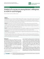
Fig. 1. RvNN, RNN, and CNN architectures.

Structure (BTS) learning scheme was introduced to train the network [47]. BTS follows an approach similar to the standard backpropagation algorithm and is also able to support a tree-like
structure. The network is trained by autoassociation to reproduce the pattern of the input layer
at the output layer.
RvNN has been especially successful in NLP. In 2011, Socher et al. [146] proposed an RvNN
architecture that can handle the inputs of different modalities. [146] shows two examples of using
RvNN to classify natural images and natural language sentences. While an image is separated into
different segments of interest, a sentence is divided into words. RvNN calculates the score of a
possible pair to merge them and build a syntactic tree. For each pair of units, RvNN computes a
score for the plausibility of the merge. The pair with the highest score is then combined into a
compositional vector. After each merge, RvNN will generate (1) a larger region of multiple units,
(2) a compositional vector representing the region, and (3) the class label (e.g., if both units are two
noun words, the class label for the new region would be a noun phrase). The root of the RvNN

tree structure is the compositional vector representation of the entire region. Figure 1(c) shows an
example RvNN tree.
2.2

Recurrent Neural Network (RNN)

Another widely used and popular algorithm in deep learning, especially in NLP and speech processing, is RNN [20]. Unlike traditional neural networks, RNN utilizes the sequential information
in the network. This property is essential in many applications where the embedded structure in
the data sequence conveys useful knowledge. For example, to understand a word in a sentence, it
is necessary to know the context. Therefore, an RNN can be seen as short-term memory units that
include the input layer x, hidden (state) layer s, and output layer y.
Figure 1(b) depicts a typical unfolded RNN diagram for an input sequence. In [124], three deep
RNN approaches including deep “Input-to-Hidden,” “Hidden-to-Output,” and “Hidden-to-Hidden”
are introduced. Based on these three solutions, a deep RNN is proposed that not only takes advantage of a deeper RNN but also reduces the difficult learning in deep networks.
ACM Computing Surveys, Vol. 51, No. 5, Article 92. Publication date: September 2018.


92:6

S. Pouyanfar et al.

One main issue of an RNN is its sensitivity to the vanishing and exploding gradients [46]. In
other words, the gradients might decay or explode exponentially due to the multiplications of lots
of small or big derivatives during the training. This sensitivity reduces over time, which means the
network forgets the initial inputs with the entrance of the new ones. Therefore, Long Short-Term
Memory (LSTM) [93] is utilized to handle this issue by providing memory blocks in its recurrent
connections. Each memory block includes memory cells that store the network temporal states.
Moreover, it includes gated units to control the information flow. Furthermore, residual connections in very deep networks [58] can alleviate the vanishing gradient issue significantly, which is
further discussed in Section 4.2.1.
2.3 Convolutional Neural Network (CNN)

CNN is also a popular and widely used algorithm in deep learning [89]. It has been extensively applied in different applications such as NLP [181], speech processing [26], and computer vision [86],
to name a few. Similar to the traditional neural networks, its structure is inspired by the neurons
in animal and human brains. Specifically, it simulates the visual cortex in a cat’s brain containing
a complex sequence of cells [67]. As described in [48], CNN has three main advantages, namely,
parameter sharing, sparse interactions, and equivalent representations. To fully utilize the twodimensional structure of an input data (e.g., image signal), local connections and shared weights
in the network are utilized, instead of traditional fully connected networks. This process results
in very fewer parameters, which makes the network faster and easier to train. This operation is
similar to the one in the visual cortex cells. These cells are sensitive to small sections of a scene
rather than the whole scene. In other words, the cells operate as local filters over the input and
extract spatially local correlation existing in the data.
In typical CNNs, there are a number of convolutional layers followed by pooling (subsampling)
layers, and in the final stage layers, fully connected layers (identical to Multilayer Perceptron
(MLP)) are usually used. Figure 1(c) shows an example CNN architecture for image classification.
The layers in CNNs have the inputs x arranged in three dimensions, m × m × r , where m refers to
the height and width of the input, and r refers to the depth or the channel numbers (e.g., r = 3 for
an RGB image). In each convolutional layer, there are several filters (kernels) k of size n × n × q.
Here, n should be smaller than the input image, but q can be either smaller or the same size as
r . As mentioned earlier, the filters are the base of local connections that are convolved with the
input and share the same parameters (weight W k and bias b k ) to generate k feature maps (hk ),
each of size m − n − 1. Similar to MLP, the convolutional layer computes a dot product between
the weights and its inputs (as illustrated in Equation (1)), but the inputs are small regions of the
original input volume. Then, an activation function f or a nonlinearity is applied to the output of
the convolutional layers:
hk = f (W k ∗ x + b k ).

(1)

Thereafter, in the subsampling layers, each feature map is downsampled to decrease the parameters in the network, speeds up the training process, and hence controls overfitting. The pooling
operation (e.g., average or max) is done over a p × p (where p is the filter size) contiguous region
for all feature maps. Finally, the final stage layers are usually fully connected as seen in the regular neural networks. These layers take previous low-level and midlevel features and generate the

high-level abstraction from the data. The last layer (e.g., Softmax or SVM) can be used to generate the classification scores, where each score is the probability of a certain class for a given
instance.

ACM Computing Surveys, Vol. 51, No. 5, Article 92. Publication date: September 2018.


A Survey on Deep Learning: Algorithms, Techniques, and Applications

92:7

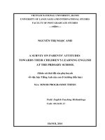
Fig. 2. The structure of generative models.

2.4 Deep Generative Networks
Here, four deep generative networks such as DBN, Deep Boltzmann Machine (DBM), Generative
Adversarial Network (GAN), and Variational Autoencoder (VAE) are discussed. DBN [61] is a hybrid probabilistic generative model in which a typical RBM with undirected connections is formed
by the top two layers, and the lower layers use directed connections to receive inputs from the
layer above. The lowest layer, which is the visible layer, represents the states of the input units as
a data vector. A DBN learns to probabilistically reconstruct its inputs in an unsupervised approach,
while the layers act as the feature detectors on the inputs. Moreover, a further training process in a
supervised way gives the DBN the capacity to perform the classification tasks. The DBN resembles
a composition of several RBMs [144], where each subnetwork’s hidden layer can be viewed as a
visible layer for the next subnetwork. Figure 2(a) illustrates the structure of a DBN.
RBMs are generative stochastic artificial neural networks that output a probability distribution
of learned inputs. An energy configuration is defined in Equation (2) to calculate the probability
distribution based on the connection weights and the unit biases by taking the state vectors v from
the visible layer:
E (v, h) = −aT v − bT h − vT Wh,

(2)


where h is the binary configuration of the hidden layer units, and a and b refer to the biases of
the visible and hidden units, respectively. A matrix W represents the connection weights between
the layers. This energy function provides a probability between each possible visible and hidden
vector pair using Equation (3):
P (v, h) =

e −E (v,h)
,
S

(3)

where S is the partition function defined as the sum of e −E (v,h) over all possible configurations
(generally, a normalizing constant to guarantee the probability distribution aggregated to 1).
The DBN includes a greedy algorithm to improve the generative model by allowing each subnetwork to sequentially receive different representations of the data, since an RBM will not be able
to model the original data ideally. Once the initial weights W0 are learned, the data can be mapped
through the transposed weighing matrix WT0 to create the higher-level “data” for the next layer. As
shown in [62], the log probability of each input data vector is bounded under the approximating
distribution. Furthermore, at each time adding a new layer into the DBN, the variational bounds
on the deeper layer are improved compared to the previous one that initializes the new RBM block
in the right direction.
Like a DBN, the DBM [135] can learn complex internal representations. It is considered as a
robust deep learning model for speech and object recognition tasks. On the other hand, unlike a
DBN, the approximate reasoning procedure allows a DBM to handle ambiguous inputs robustly.
Figure 2(b) presents the architecture of a DBM, which is a composite model of RBMs. It also clearly
ACM Computing Surveys, Vol. 51, No. 5, Article 92. Publication date: September 2018.


92:8


S. Pouyanfar et al.

shows how a DBM differs from a DBN. The lower layers in a DBN build a directed belief network,
instead of the undirected RBMs as in a DBM.
The layer-wise greedy training algorithm for a DBM can be easily calculated by modifying the
procedure in a DBN. A factorial approximation to the posterior can take either the result from
the first RBM or the probability from the second layer. Taking a geometric average of these two
distributions would be a better idea to balance the approximations to the posterior, which uses
1/2 W0 bottom-up and 1/2 W1 (the second layer weights) top-down.
GAN [49] consists of a generative model G and a discriminative model D. While G captures
the distribution pд over the real data t locally, D tries to differentiate a sample that comes from
the modeling data m rather than pд , represented by pm . In every iteration of the backpropagation,
the generator and the discriminator, like in a game of cat and mouse, compete between each
other. While the generator is trying to generate more realistic data to fool and confuse the
discriminator, the latter tries to identify the real data from the fake ones that were generated by
G. The two-player minimax game is established with a value function V (G, D):
min max V (G, D) = Et ∼pdata [loдD (t )] + Em∼pm (m)) [loд(1 − D(G (m)))],
G

D

(4)

where D(t ) represents the probability that t came from the data rather than pд , and pdata is the
distribution of the real-world data. The model is considered to be stable when both reach the
point where none of them can be improved, as pд = pdata . That is, the discriminator can no longer
identify between the two distributions. Figure 2(c) shows a GAN architecture.
Another famous generative model is VAE [81]. An example VAE architecture is given in
Figure 2(d). It utilizes the log-likelihood of the data and leverages the strategy of deriving a lower
bound estimator from the directed graphical models with continuous latent variables. The generative parameters θ in the generative model assist the learning process of the variational parameters

ϕ in the variational approximation model. The Auto-Encoding Variational Bayes (AEVB) algorithm
optimizes the parameters ϕ and θ for the probabilities encoder qϕ (z|x ) in the neural network,
which is an approximation to the generative model pθ (x, z), where z is the latent variable under a
simple distribution, i.e., N (0, I ), and I is the identity matrix. It aims to maximize the probability of
each x in the training set under the entire generative process:
pθ (x ) =

pθ (z)pθ (x |z)dz.

(5)

3 DEEP LEARNING TECHNIQUES AND FRAMEWORKS
Different deep learning algorithms help improve the learning performance, broaden the scopes of
applications, and simplify the calculation process. However, the extremely long training time of the
deep learning models remains a major problem for the researchers. Furthermore, the classification
accuracy can be drastically enhanced by increasing the size of training data and model parameters.
In order to accelerate the deep learning processing, several advanced techniques are proposed in
the literature. Deep learning frameworks combine the implementation of modularized deep learning algorithms, optimization techniques, distribution techniques, and support to infrastructures.
They are developed to simplify the implementation process and boost the system-level development and research. In this section, some of these representative techniques and frameworks are
introduced.
3.1 Unsupervised and Transfer Learning
Contrary to the vast amount of work done in supervised deep learning, very few studies have
addressed the unsupervised learning problem in deep learning. However, in recent years, the
ACM Computing Surveys, Vol. 51, No. 5, Article 92. Publication date: September 2018.


A Survey on Deep Learning: Algorithms, Techniques, and Applications

92:9


benefit of learning reusable features using unsupervised techniques has shown promising results
in different applications. In the last decade, the idea of having a self-taught learning framework
has been widely discussed in the literature [88, 130, 140].
In recent few years, generative models such as GANs and VAEs have become dominant techniques for unsupervised deep learning. For instance, GANs are trained and reused as a fixed feature extractor for supervised tasks in [130]. This network is based on CNNs and has shown its
supremacy as unsupervised learning in visual data analysis. In another work, a deep sparse Autoencoder is trained on a very large-scale image dataset to learn features [88]. This network generates a high-level feature extractor from unlabeled data, which can be used for face detection in an
unsupervised manner. The generated features are also discriminative enough to detect other highlevel objects like animal faces or human bodies. Bengio et al. [11] propose a generative stochastic
network for unsupervised learning as an alternative to the maximum likelihood that is based on
transition operators of Markov chain Monte Carlo.
In practice, very few people have the luxury of accessing very high-speed GPUs and powerful
hardware to train a very deep network from scratch in a reasonable time. Therefore, pretraining a
deep network (e.g., CNN) on large-scale datasets (e.g., ImageNet) is very common. This technique
is also known as transfer learning [157], which can be done by using the pretrained networks
as fixed feature extractors (especially for small new datasets) or fine-tuning the weights of the
pretrained model (especially for large new datasets that are similar to the original one). In the
latter, the model should continue the learning to fine-tune the weights of all or some of the highlevel parts of the deep network. This approach can be considered as a semisupervised learning, in
which the labeled data is insufficient to train a whole deep network.
3.2

Online Learning

Usually, the network topologies and architectures in deep learning are time static (i.e., they are
predefined before the learning starts) and are also time invariant [90]. This restriction on time
complexity poses a serious challenge when the data is streamed online. Online learning previously came into mainstream research [21], but only a modest advancement has been observed in
online deep learning. Conventionally, DNNs are built upon the Stochastic Gradient Descent (SGD)
approach in which the training samples are used individually to update the model parameters with
a known label. The need is that rather than the sequential processing of each sample, the updates
should be applied as batch processing. One approach was presented in [137] where the samples
in each batch are treated as Independent and Identically Distributed (IID). The batch processing
approach proportionally balances the computing resources and execution time.
Another challenge that stacks up on the issue of online learning is high-velocity data with timevarying distributions. This challenge represents the retail and banking data pipelines that hold

tremendous business values. The current premise is that the data is largely close in time to safely
assume piecewise stationarity, thus having a similar distribution. This assumption characterizes
data with a certain degree of correlation and develops the models accordingly, as discussed in
[19]. Unfortunately, these nonstationary data streams are not IID and are often longitudinal data
streams. Moreover, online learning is often memory delimited, is harder to parallelize, and requires
a linear learning rate on each input sample. Developing methods that are capable of online learning
from non-IID data would be a big leap forward for big data deep learning.
3.3 Optimization Techniques in Deep Learning
Training a DNN is an optimization process, i.e., finding the parameters in the network that minimize the loss function. In practice, the SGD method [150] is a fundamental algorithm applied to
deep learning, which iteratively adjusts the parameters based on the gradient for each training
ACM Computing Surveys, Vol. 51, No. 5, Article 92. Publication date: September 2018.


92:10

S. Pouyanfar et al.

sample. The computational complexity of SGD is lower than that of the original gradient descent
method, in which the whole dataset is considered every time the parameters are updated.
In the learning process, the updating speed is controlled by the hyperparameter learning rate.
Lower learning rates will eventually lead to an optimal state after a long time, while higher learning
rates decay the loss faster but may cause fluctuations during the training [128]. In order to control
the oscillation of SGD, the idea of using momentum is introduced. Inspired by Newton’s first law
of motion, this technique gets a faster convergence and a proper momentum that can improve the
optimization results of SGD [150].
On the other hand, several techniques are proposed to determine the proper learning rate. Primitively, weight decay and learning rate decay are introduced to adjust the learning rate and accelerate the convergence. A weight decay works as a penalty coefficient in the cost function to avoid
overfitting, and a learning rate decay can reduce the learning rate dynamically to improve the
performance. Moreover, adapting the learning rate with respect to the gradient of the previous
stages is found helpful to avoid the fluctuation. Adagrad [35] is the first adaptive algorithm successfully used in deep learning. It amplifies the learning rate for infrequently updated parameters
and suppresses the learning rate for the frequently updated parameters by recording the accumulated squared gradients. Since the squared gradients are always positive, the learning rate of

Adagrad can become extremely small and does not optimize the model anymore. To solve this issue, Adadelta [176] is proposed, where a decay fraction β 2 is introduced to limit the accumulation
of the squared gradients as follows:
E[д2 ]t = β 2 E[д2 ]t −1 + (1 − β 2 )дt2 ,

(6)

where E[д2 ]t is the accumulated squared gradient at stage t and дt2 is the squared gradient at stage
t. Later, the Adadelta is further improved by introducing another decay fraction β 1 to record the
accumulation of the gradients [80]. It is shown that Adam performs better in practice than the
other algorithms with an adaptive learning rate. AdaMax is also proposed in the same paper as an
extension of Adam, where the l − 2 norm used in Adam is replaced by the l − inf norm to achieve
a stable algorithm. Adam can also incorporate with Nesterov Accelerated Gradient (NAG), called
NAdam [34]. It shows better convergence speed in some cases.
3.4 Deep Learning in Distributed Systems
The efficiency of model training is limited to a single-machine system, and the distributed deep
learning techniques have been developed to further accelerate the training process. There are
two main approaches to train the model in a distributed system, namely, data parallelism and
model parallelism. For data parallelism, the model is replicated to all the computational nodes and
each model is trained with the assigned subset of data. After a certain period of time, the weight
update needs to be synchronized among the nodes. Comparatively, for model parallelism, all the
data is processed with one model where each node is responsible for the partial estimation of the
parameters in the model.
Among data-parallel approaches, the most straightforward algorithm to combine results from
the slave nodes is parameter averaging [108]. Let Wt,i be the parameter in a neural network on
node i at time t with N slave nodes used for training. At time t, the weight on the master node
is Wt . Then, a copy of the current parameters is distributed to the slave nodes. After the updated
parameters are sent back to the master node, the weight at time t + 1 on the master node will be
Wt +1 =

1

N

N

Wt +1,i .
i=1

ACM Computing Surveys, Vol. 51, No. 5, Article 92. Publication date: September 2018.

(7)


A Survey on Deep Learning: Algorithms, Techniques, and Applications

92:11

Parameter averaging would be identical to single-machine training if parameters are averaged after each minibatch and if each worker processes the same number of data copies. However, the
network communication and synchronization costs can nullify the benefits of extra machines.
Therefore, the averaging process is usually applied after a certain number of minibatches are fed
to each slave node. The frequency of training and the model performance need to be balanced as
required. A more popular approach for data parallelism uses SGD and is known as update-based
data parallelism [149], where the updates of the learning rate decay and momentum are transferred. However, the synchronous weight update is not scalable for a larger cluster. The overhead
of communication increases exponentially with respect to the number of nodes. Therefore, a parameter server framework is proposed by Google to process the training asynchronously [92].
Instead of waiting for the parameter to be updated on the master node, the asynchronous update
allows each node to spend more time on computation. Meanwhile, the network communication
cost can be significantly reduced by decentralization, i.e., transmitting the updates in peer-to-peer
mode instead of master-slave mode.
On the other hand, a model parallelism approach splits the training step across multiple GPUs.
In a straightforward model-parallel strategy, each GPU computes only a subset of the model. For
example, for a model with two LSTM layers, the system with two GPUs can use each of them to

calculate one LSTM layer. The advantage of the model-parallel strategy is that it makes training and
prediction with massive deep neural networks possible [28]. For instance, the COTS HPC system
trained a neural network with more than 11 billion parameters, which requires about 82GB of
memory [24]. It is impossible to fit such a large model into one machine and therefore it needs to be
partitioned using model-parallel strategies. However, since the model is partitioned across nodes,
one drawback of model parallelism is that each node can only compute a subset of results [8] and
synchronization is thus needed to get the full results. The synchronization loss and communication
overhead of model-parallel strategies are more than those of data-parallel strategies since each
node in the former must synchronize both gradients and parameter values on every update step.
In other words, the scalability of model parallelism is inferior. To handle this issue, Google has
proposed an automated device placement framework based on deep reinforcement learning to find
the best scheme of the model partition and placement [110]. The framework takes the embedding
representation of each operation, places the grouped operations to different devices, and shows a
60% performance improvement compared to the human experts.
Both data-parallel and model-parallel strategies have their own limitations. On one hand, if data
parallelism has too many training modules, it has to decrease the learning rate to make the training procedure smooth. On the other hand, if model parallelism has too many segmentations, the
output from the nodes will increase sharply and reduce the efficiency accordingly [168]. Generally
speaking, the larger the dataset is, the more beneficial it is to have data parallelism. The larger the
deep learning model is, the more suitable it is to have model parallelism. Besides, compared to data
parallelism, it is hard to hide the communication needed for synchronization in model parallelism
because only partial information is included in each node for the whole batch, though some advanced frameworks like TensorFlow[1] support asynchronous kernels to save the communication
cost. Thus, it is necessary to wait till the synchronization step finishes before moving forward to
the next layer since the activities are unable to be processed with only partial information. The
two kinds of strategies can also be fused to a hybrid model as discussed in [168].
3.5 Deep Learning Frameworks
Table 2 lists a smattering of popular deep learning frameworks for architecture designs, such
as Caffe [72], DeepLearning4j (DL4j) [143], Torch [25], Neon [69], Theano [5], MXNet [17],
TensorFlow [1], and Microsoft Cognitive Toolkit (CNTK) [173]. In Table 2, the license, core
ACM Computing Surveys, Vol. 51, No. 5, Article 92. Publication date: September 2018.



92:12

S. Pouyanfar et al.
Table 2. The Comparison of Different Deep Learning Frameworks

Framework

License

Core
Language

Caffe [72]

BSD

C++

DL4j [143]

Apache 2.0

Java

Torch [25]

BSD

C & Lua


Neon [69]
Theano [5]

Apache 2.0
BSD

Python
Python

MXNet [17]

Apache 2.0

C++

TensorFlow
[1]

Apache 2.0

C++ &
Python

CNTK [173]

MIT

C++


Interface
Support
Python &
MATLAB
Java, Scala, &
Python
C/C++, Lua, &
Python
Python
Python
C++, Python,
R, Scala, Perl,
Julia, etc.
Python,
C/C++, Java,
& Go
Python, C++,
& BrainScript

CNN & RNN
Support

DBN
Support

Yes

No

Yes


Yes

Yes

Yes

Yes
Yes

Yes
Yes

Yes

Yes

Yes

Yes

Yes

No

language, supported interface language, and framework support of CNN, RNN, and DBN are also
listed.
It can be observed from Table 2 that C++ is usually used for implementation of deep learning
frameworks because it accelerates the speed of training. Since GPU is significantly helpful to speed
up the matrix computation, most of the aforementioned frameworks also support GPU via the interface provided by CuDNN [18]. Meanwhile, Python has become the most common language for

deep learning architecture design since it can make the programming more efficient and easier by
simplifying the programming process. Also, distributed calculation becomes common in some recently released frameworks such as TensorFlow, MXNet, and CNTK. The goal is to further improve
the calculation efficiency for deep learning. Moreover, TensorFlow also includes support for the
customized deep learning Application-Specific Integrated Circuit (ASIC), called Tensor Processing
Unit (TPU), to help increase the efficiency and decrease the power consumption.
Caffe, implemented by Berkeley Vision and Learning Center, is one of the most widely used
frameworks [72]. It supports the most commonly used layers for both CNN and RNN but does not
directly enable the use of DBN. Users of Caffe design their architecture by declaring the structure
of a computation graph, such as convolutional layers. There are pretrained models available for
a wide range of neural networks such as AlexNet [86], GoogleNet [151], and ResNet [58]. Furthermore, Caffe is a single-machine framework. In other words, it does not support multinode
execution while the multi-GPU calculation is supported when there are external offerings like
CaffeOnSpark by Yahoo that integrate Caffe with a big data engine like Spark.
DL4j is the most popular framework implemented in Java, developed and maintained by Skymind since 2014 [143]. Cooperating with Hadoop and Spark, DL4j is capable of distributed computation as well. However, this framework is reported to have a longer training time for similar
architectures benchmarked with other frameworks [84].
Torch was first released in 2002 and extended its deep learning feature in 2011 [25]. Combined
with Facebook’s deep learning CUDA library (fbcunn) [160], Torch can operate model- and
ACM Computing Surveys, Vol. 51, No. 5, Article 92. Publication date: September 2018.


A Survey on Deep Learning: Algorithms, Techniques, and Applications

92:13

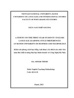
Fig. 3. Some of the popular deep learning applications.

data-level parallel computation. Unlike other frameworks, Torch is built based on a dynamic
graph representation instead of a static graph. The dynamic graph allows the user to update
the computational graph (i.e., to change the model structure) during runtime, while the static
graph uses certain functions to define the graphs in advance. Recently, Torch released its Python
interface, PyTorch, and the usage of this framework has greatly increased due to its flexibility.

Neon [69] and Theano [5] are two frameworks developed in Python by Intel and the University of Montreal, respectively. Both of them perform code optimizations in the system and kernel
level. Therefore, their training speeds usually outperform other frameworks. However, although
only parallelism and multi-GPU are supported, the multinode calculation is not designed in these
frameworks.
MXNet supports several interfaces, including C++, Python, R, Scala, Perl, MATLAB, Javascript,
Go, and Julia [17]. It supports both computation graph declarations and imperative computation
declarations for architecture design. MXNet not only supports data and model parallelism but also
follows parameter server schemes to support distributed calculation as well. MXNet has the most
comprehensive functionality, but the performance is not optimized as much as other state-of-theart frameworks.
TensorFlow is implemented by Google and provides a series of internal functions to help implement any deep neural network based on the static computational graph [1]. Recently, Keras started
to support Tensorflow via a high-level interface and allowed users to design the architecture without worrying about the internal design. The framework provides different levels of parallel and
distributed operations and well-designed fatal tolerance. The robustness of its design attracts a lot
of users and it has become one of the most popular deep learning frameworks since its release.
CNTK, designed by Microsoft, has a specific high-level script language, BrainScript, for neural
network implementation [173]. CNTK models the neural network as a directed graph. Each node
in the graph represents an operation or a filter and each edge refers to the data flow. Instead of
the parameter server model, the Message Passing Interface is applied for distributed calculation
support.
4 VARIOUS APPLICATIONS OF DEEP LEARNING
Nowadays, applications of deep learning include but are not limited to NLP (e.g., sentence classification, translation, etc.), visual data processing (e.g., computer vision, multimedia data analysis,
etc.), speech and audio processing (e.g., enhancement, recognition, etc.), social network analysis,
and healthcare. This section provides details for the different techniques used for each application.
Some of the main deep learning applications are also visualized in Figure 3.
ACM Computing Surveys, Vol. 51, No. 5, Article 92. Publication date: September 2018.


92:14

S. Pouyanfar et al.
Table 3. Popular Deep Learning Methods in NLP


Paper
Socher et al. 2013 [147]

Wehrmann et al. 2017 [164]

NLP Tasks
Sentiment Analysis
Sentiment Analysis,
General Classification
Sentiment Analysis

Bahdanau et al. 2014 [9]

Translation

Cho et al. 2014 [20]

Translation

Wu et al. 2016 [166]

Translation

GNMT

Socher et al. 2011 [145]

Paraphrase Identification
Paraphrase Identification,

Question & Answer
Summarization
Question & Answer
Question & Answer

Unfolding RAE

Kim 2014 [79]

Yin et al. 2015 [172]
Kågebäck et al. 2014 [75]
Dong et al. 2015 [33]
Feng et al. 2015 [39]

Architecture
RNTN

Datasets
SST

CNN

SST

Conv-Char-S
Bidir RNN
EncoderDecoder
RNN EncoderDecoder

MTD


ABCNN
Unfolding RAE
MCCNN
CNN

WMT-14-EF
WMT-14-EF
WMT-14-EF
WMT-14-EG
MSRP
WikiQA
MSRP
OD
WQ
IQA

4.1 Natural Language Processing
NLP is a series of algorithms and techniques that mainly focus on teaching computers to understand the human language. Some NLP tasks include document classification, translation, paraphrase identification, text similarity, summarization, and question answering. NLP development
is challenging due to the complexity and ambiguous structure of the human language. Moreover,
natural language is highly context specific, where literal meanings change based on the form of
words, sarcasm, and domain specificity. Deep learning methods have recently been able to demonstrate several successful attempts in achieving high accuracy in NLP tasks. Table 3 contains a summary for some of the leading deep learning NLP solutions, their architectures, and their datasets.
Most NLP models follow a similar preprocessing step: (1) the input text is broken down into words
through tokenization and then (2) these words are reproduced in the form of vectors, or n-grams.
Representing words in a low dimension is important to create an accurate perception of similarities and differences between various words. The challenge arrives when there is a need to decide
the length of words contained in each n-gram. This procedure is context specific and requires prior
domain knowledge. Some of the highly impactful approaches in solving the most well-known NLP
tasks are presented below.
4.1.1 Sentiment Analysis. This branch of NLP deals with examining a text and classifying the
feeling or opinion of the writer. Most datasets for sentiment analysis are labeled as either positive

or negative, and neutral phrases are removed by subjectivity classification methods. One popular
example is the Standford Sentiment Treebank (SST) [147], a dataset of movie reviews labeled in
five categories (ranging from very negative to very positive). Along with the introduction to SST,
Socher et al. [147] propose a Recursive Neural Tensor Network (RNTN) that utilizes word vectors
and parses a tree to represent a phrase, capturing the interactions between the elements with a
tensor-based composition function. This recursive approach is advantageous when it comes to
sentence-level classification since the grammar often displays a tree-like structure.
ACM Computing Surveys, Vol. 51, No. 5, Article 92. Publication date: September 2018.


A Survey on Deep Learning: Algorithms, Techniques, and Applications

92:15

Kim [79] improves the accuracy for SST by following a different approach. Even though CNN
models were first created with image recognition and classification in mind, their implementation
in NLP has proven to be a success, achieving excellent results. Kim presents a simple CNN model
using one convolution layer on top of trained word2vec vectors in a BoW architecture. The models
were kept relatively simple with a small number of hyperparameters for tuning. By a combination
of low tuning and pretrained task-specific parameters, they managed to achieve high accuracy
on several benchmarks. Social media is a popular source of data when studying sentiments. The
Multilingual Twitter Dataset (MTD) [114] is one of the largest public datasets, containing over
1.6 million manually annotated tweets in 13 languages. Applying sentiment analysis to tweets is
challenging due to the short nature of the text. To address the issue of a multilingual dataset with
a small amount of text, [164] proposes Conv-Char-S, a character-based architecture that is exempt
from dependence on languages. Although the approach was not capable of outperforming wordembedding architectures, the authors argue its simplicity and predictive power consumption to be
a good tradeoff.
4.1.2 Machine Translation. Deep learning has played an important role in the improvements
of traditional automatic translation methods. Cho et al. [20] introduced a novel RNN-based encoding and decoding architecture to train the words in a Neural Machine Translation (NMT).
The RNN Encoder-Decoder framework uses two RNNs: one maps an input sequence into fixedlength vectors, while the other RNN decodes the vector into the target symbols. The downside

to the RNN Encoder-Decoder is the performance deterioration as the input sequence of symbols
becomes larger. Bahdanau et al. [9] address this issue by introducing a dynamic-length vector
and by jointly learning the align and translate procedures. Their approach is to perform a binary
search to look for parts of speech that are most predictive for the translation. Nonetheless, the
recently proposed translation systems are known to be computationally expensive and inefficient
in handling sentences containing rare words. Thus, in [166], Google’s Neural Machine Translation
(GNMT) system is proposed, introducing a balance between the flexibility provided by characterlevel models and the efficiency of word-level models. GNMT is a deep LSTM network that makes
use of eight encoder and eight decoder layers connected using the attention-based mechanism.
The attention-based method was first introduced to improve NMT in general. The model achieved
the state-of-the-art scores in WMT’14 English-to-French and English-to-German benchmarks.
4.1.3 Paraphrase Identification. Paraphrase identification is the process of analyzing two sentences and projecting how similar they are based on their underlying hidden semantics. It is a key
feature that is beneficial for several NLP jobs such as plagiarism detection, answers to questions,
context detection, summarization, and domain identification. Socher et al. [145] propose the use
of unfolding Recursive Autoencoders (RAEs) to measure the similarity of two sentences. Using
syntactic trees to develop the feature space, they measure both word- and phrase-level similarities. Even though it is very similar to RvNN, RAE is useful in unsupervised classification. Unlike
RvNN, RAE computes a reconstruction error instead of a supervised score during the merging of
two vectors into a compositional vector. The paper also introduced a dynamic pooling layer that
can compare and classify two sentences of different sizes as either a paraphrase or not. Several
other notable methods were investigated by [31] for monolingual phrase-level semantic similarity
detection. They also enlist some of the most notable datasets in paraphrase identification, e.g., the
Microsoft Research Paraphrase Corpus (MSRP) and the Topically Clustered News Article dataset.
Attention-Based CNN (ABCNN) is a recently proposed deep learning architecture with the goal of
determining the interdependence between two sentences [172]. Other than paraphrase detection,
it has also been applied to answer selection and textual entailment.

ACM Computing Surveys, Vol. 51, No. 5, Article 92. Publication date: September 2018.


92:16


S. Pouyanfar et al.

4.1.4 Summarization. Automatic summarization can extract the most significant and relevant
information from large text documents. A well-represented summary effectively reduces the size
of text without losing the most important information. This can considerably decrease the time
and computations required to analyze large text-based datasets. Kågebäck et al. [75] propose a
continuous vector representation-based model for the sentences. Their model evaluates multiple
combinations and compositions for meaningful representations. The new vector representation
is tested using RAE compared with simple vector addition. The paper makes use of the ROUGE
benchmarking metrics to evaluate the effectiveness of their summarization framework. Ganesan
et al. [41] utilize a graph-based model that produces brief summaries from the opinion dataset
known as Opinosis Dataset (OD). Their model targets user opinions in terms of feedback, product
reviews, and customer satisfaction reports without losing any educative material.
4.1.5 Question Answering. An automatic question-and-answering system should be able to interpret a natural language question and use reasoning to return an appropriate reply. Modern
knowledge bases, such as the famous FREEBASE dataset, allow this field to flourish and leap out
of the times when features and rule sets were hand-crafted to specific domains. Dong et al. [33]
came up with a multicolumn CNN approach that can analyze a question from several aspects,
i.e., which context to choose, underlying semantic meaning of the answer, and how to form the
answer. They use a multitasking approach that ranks the question-answer pairs and also simultaneously learns the correlations and affiliations of the low-level word semantics. A more general
deep learning architecture that is not limited to any one language is proposed [39]. The Question Answering (QA) framework proposed by the paper is based on CNN and uses a corpus-based
approach to answer questions in the insurance domain. They test many different setups of a CNNbased architecture and compare the results. Berant et al. [12] propose a highly scalable version of
the question-answer model. Their solution to the problem of large datasets is to avoid the logical
forms of text and learn the model solely on question-answer tuples. ABCNN [172] proves its capability in the Question-and-Answering NLP task by ranking the candidate answers based on how
closely they were interdependent to the question. The datasets used by the papers mentioned in
this section are Web Questions (WQ), Insurance Question Answering (IQA), and WikiQA.
4.2 Visual Data Processing
Deep learning techniques have become the main parts of various state-of-the-art multimedia systems and computer vision [54]. More specifically, CNNs have shown significant results in different
real-world tasks, including image processing, object detection, and video processing. This section
discusses more details about the most recent deep learning frameworks and algorithms proposed
over the past few years for visual data processing.

4.2.1 Image Classification. In 1998, LeCun et al. presented the first version of LeNet-5 [91].
LeNet-5 is a conventional CNN that includes two convolutional layers along with a subsampling
layer and finally ending with a full connection in the last layer. Although, since the early 2000s,
LeNet-5 and other CNN techniques were greatly leveraged in different problems, including the
segmentation, detection, and classification of images, they were almost forsaken by data mining
and machine-learning research groups. More than one decade later, the CNN algorithm has started
its prosperity in computer vision communities. Specifically, AlexNet [86] is considered the first
CNN model that substantially improved the image classification results on a very large dataset
(e.g., ImageNet). It was the winner of the ILSVRC 2012 and improved on the best results from the
previous years by almost 10% regarding the top five test error. To improve the efficiency and the
speed of training, a GPU implementation of the CNN is utilized in this network. Data augmentation
and dropout techniques are also used to substantially reduce the overfitting problem.
ACM Computing Surveys, Vol. 51, No. 5, Article 92. Publication date: September 2018.


A Survey on Deep Learning: Algorithms, Techniques, and Applications

92:17

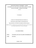
Fig. 4. The network top five errors (%) and layers in the ImageNet classification over time.

Since then, a variety of CNN methods have been developed and submitted to the ILSVRC competition. In 2014, two influential but different models were presented that mostly focused on the depth
of neural networks. The first one, known as VGGNet [142], includes a very simple 19-layer CNN. In
this network, at each layer, the spatial size of the input is reduced, while the depth of the network is
increased to achieve a more effective and efficient model. Although VGGNet was not the winner of
the ILSVRC 2014, it still shows a significant improvement (7.3% top five error) over the previous top
models that came from its two major specifications: simplicity and depth. In contrast to VGGNet,
GoogleNet [151], the winner of this competition (6.7% error), proposed a new complex module
named “Inception,” allowing several operations (pooling, convolutional, etc.) to work in parallel.
The Microsoft deep residual network (known as ResNet) [58] took the lead in the 2015 competitions including ILSVRC 2015 and in COCO detection and segmentation tasks by introducing the

residual connections in CNNs and designing an ultra-deep learning model (50 to 152 layers). This
model achieved an incredible performance (3.6% top five error), which means, for the first time, a
computer model could beat human brains (with 5% to 10% error) in image classification. Contrary
to the extremely deep representation of ResNet, it can handle the vanishing gradients [46] as well
as the degradation problem (saturated accuracy) in deep networks by utilizing residual blocks.
In the last few years, several variations of ResNet have been proposed. The first group of methods
has tried to increase the number of layers more and more. Current CNN models may include more
than 1,000 layers [64]. Finally, in 2017, ResNeXT [167] was proposed as an extension of ResNet
and VGGNet. This simple model includes several branches in a residual block, each performing
a transformation that is finally aggregated by a summation operation. This general model can be
further reshaped by other techniques such as AlexNet. ResNeXT outperforms its original version
(ResNet) using half of the layers and also improves the Inception-v3 as well as Inception-ResNet
networks on the ImageNet dataset. Figure 4 demonstrates the revolution of depth and performance
in image classification (e.g., ImageNet) over time. The problem of supervised image classification
is regarded as “solved” and the ImageNet classification challenge concluded in 2017.
4.2.2 Object Detection and Semantic Segmentation. Deep learning techniques play a major
role in the advancement of object detection in recent years. Before that, the best object detection
performance came from complex systems with several low-level features (e.g., SIFT, HOG, etc.)
and high-level contexts. However, with the advent of new deep learning techniques, object
detection has also reached a new stage of advancement. These advances are driven by successful
methods such as region proposal and Region-based CNN (R-CNN) [45]. R-CNN bridges the
ACM Computing Surveys, Vol. 51, No. 5, Article 92. Publication date: September 2018.


92:18

S. Pouyanfar et al.

gap between the object detection and image classification by introducing region-based object
localization methods using deep networks. In addition, transfer learning and pertaining on a large

dataset (e.g., ImageNet) is utilized since the small object detection datasets (e.g., PASCAL [123])
include insufficient labeled data to train a large CNN network. However, in R-CNN, the training
computational time and memory are very expensive, especially on new ultra-deep networks (e.g.,
VGGNet). Moreover, the object detection step is very slow. Later, this technique is extended to
overcome the aforementioned issues by introducing two successful techniques: Fast R-CNN [44]
and Faster R-CNN [133]. The former leverages sharing computation to speed up the original
R-CNN and train a very deep VGGNet, while the latter proposes a Region Proposal Network
(RPN) that enables almost real-time object detection.
A real-time object detection is called YOLO (You Only Look Once) [132], which contains a single
CNN. The convolutional network performs bounding-box detection and class probability calculation for each box simultaneously. The benefits of YOLO include its fast training and testing (45
frames per second) and its reasonable performance compared to previous real-time systems.
Unlike Fast/Faster R-CNN, a recent method called Region-based Fully Convolutional Networks
(R-FCNs) [95] utilizes a fully convolutional network that shares almost all computations on an
image. This method uses the ResNet classifier as an object detector and achieves a test-time speed
faster than the Faster R-CNN method. Finally, the Single-Shot MultiBox Detector (SSD) [100] is
proposed, which is faster than YOLO, and its performance is as accurate as region-based techniques
such as Faster R-CNN. Its model is based on a single CNN that generates a set of bounding boxes
with fixed sizes as well as the corresponding object scores in the boxes.
Semantic segmentation is the process of understanding an image in pixel level that is necessary
for real-world applications such as autonomous driving, robot vision, and medical systems. Now
the question is how to convert image classification to semantic segmentation. In recent years,
many research studies apply deep learning techniques to classify an image pixel-wise. A deconvolutional network [122], for instance, includes deconvolution and unpooling modules to detect and
classify the segmentation regions. In another work, a Fully Convolutional Network (FCN) [101]
is proposed and utilizes networks such as AlexNet, VGGNet, and GoogleNet. Recently, Mask
R-CNN was proposed by Facebook AI Research (FAIR) [57] for object instance segmentation. It
extends Faster R-CNN by adding a new branch that generates the segmentation mask prediction
for each region of interest at the same time that the bounding box and class label are generated.
This simple and flexible model has shown great performance results in both COCO instance
segmentation and object detection.
4.2.3 Video Processing. Video analytics has attracted considerable attention in the computer

vision community and is considered as a challenging task since it includes both spatial and temporal information. In an early work, large-scale YouTube videos containing 487 sport classes are
used to train a CNN model [77]. The model includes a multiresolution architecture that utilizes the
local motion information in videos and includes context stream (for low-resolution image modeling) and fovea stream (for high-resolution image processing) modules to classify videos. An event
detection from sport videos using deep learning is presented in [159]. In that work, both spatial
and temporal information are encoded using CNNs and feature fusion via regularized Autoencoders. In recent years, a new technique called Recurrent Convolution Networks (RCNs) [32] was
introduced for video processing. It applies CNNs on video frames for visual understanding and
then feeds the frames to RNNs for analyzing temporal information in videos. A new RCN model
proposed in [10] uses RNN on the intermediate layers of CNNs. In addition, a Gated Recurrent
Unit is used to leverage the sparsity and locality in the RNN modules. This model is validated on
the UCF-101 and YouTube2Text datasets.
ACM Computing Surveys, Vol. 51, No. 5, Article 92. Publication date: September 2018.


A Survey on Deep Learning: Algorithms, Techniques, and Applications

92:19

Table 4. Popular Visual Datasets for Deep Learning

Dataset

Data
Type

Num of Num of
Instances Classes

ImageNet [68]

Images


14M

1,000

CIFAR10/100 [22]

Images

60K

10/100

Pascal VOC [123]

Images

46K

20

Microsoft COCO
[96]

Images

2M

80


MNIST [112]

Images

70K

10

100M

8M

8M

4,716

YouTube-8M [4]

Images
Videos
Videos

Trecvid [158]

Videos

Varies

Varies


UCF-101 [148]
Kinetics [78]

Videos
Videos

13K
306K

101
400

YFCC100M [152]

Ground
Truth

Applications

Image classification,
object localization, object
detection, etc.
Yes
Image classification
Image classification,
Yes
object detection, semantic
segmentation
Object detection, semantic
Yes

segmentation
Handwritten digit,
Yes
classification
Video and image,
Partially
understanding
Automatic
Video classification
Video search, event
Partially
detection, localization, etc.
Yes
Human action detection
Yes
Human action detection
Yes

Three-dimensional CNN (C3D) [156] has demonstrated a better performance on video analysis
tasks over the traditional 2D CNNs. It automatically learns spatiotemporal features from video
inputs and models the appearance and motions at the same time. Two-stream networks [38] are
another set of video analysis techniques that model spatial (RGB frame) and temporal information
(optical flow) separately and average the predictions in the last few layers of the network. This
network is extended in a recent work called Inflated 3D ConvNet (I3D), utilizing the idea of C3D. It
is also pretrained on the Kinetics dataset [78]. The proposed approach could significantly enhance
the performance of action recognition in UCF-101 and HMDB-51 datasets.
4.2.4 Visual Datasets. The significant advancements in image and video processing not only
rely on the development of new learning algorithms and utilization of powerful hardware but
also crucially depend on very large-scale public datasets. Several large-scale visual datasets used
to train deep learning algorithms are listed in Table 4. ImageNet [68] can be considered as the

most important and influential dataset in deep learning. It is used to train all popular networks
such as AlexNet, GoogleNet, VGGNet, and ResNet due to its large-scale labeled image collections.
A smaller-scale image dataset that is utilized in many research studies is CIFAR10/100 [22]. This
dataset is also used for evaluating many DNNs in the image classification task. As mentioned
earlier, PASCAL VOC and Microsoft COCO are used for various object detection and semantic
segmentation tasks. Finally, YouTube-8M [4] is a relatively new dataset generated by Google to
play the same role as ImageNet for video processing. It can be utilized as a benchmark dataset for
various video analyses, including event detection, understanding, and classification.
4.3 Speech and Audio Processing
Audio processing is the process that operates directly on electrical or analog audio signals. It is necessary for speech recognition (or speech transcription), speech enhancement, phone classification,
ACM Computing Surveys, Vol. 51, No. 5, Article 92. Publication date: September 2018.


92:20

S. Pouyanfar et al.

and music classification. Speech processing is an active research area because of its importance
in perfect human-computer interaction. From the 1970s till the 21st century, Automatic Speech
Recognition (ASR) [74] technology has risen to an unprecedented level. However, it is still far from
mimicking human-like behavior to communicate with human beings. An ASR system is made up
of many components, including speech signal preprocessing, feature extraction, acoustic modeling, phonetic unit recognition, and language modeling. The traditional ASR systems integrate the
Hidden Markov Models (HMMs) with the Gaussian Mixture Models (GMMs). The HMMs are used
to deal with the variation of speech, which is related to the time space, while the GMMs represent
the acoustic characteristics of sound units. The modeling process is time-consuming and requires
a very large training dataset in order to reach a high accuracy. The ANNs [60] were introduced
during the 1980s, which are composed of many nonlinear computational elements operating in
parallel. However, deeper architectures with multiple layers are needed to settle the limitation of
GMMs on sufficiently representing HMMs. DBN, one of the commonly used deep learning models
in this area, significantly improves the performance of the acoustic models. It models the spectral

variations in speech with RBMs as their building blocks. Seide et al. [139] use pretrained DBNs
and demonstrate the strength of their model on a publicly available benchmark, the Switchboard
phone-call transcription task. They introduce weight sparseness and the related learning strategy
to reduce the recognition error and model size. Followed by the widely studied DBN pretraining
method, Dahl et al. [26] propose a novel acoustic model for Large-Vocabulary-Speech-Recognition
(LVSR). The model integrates a pretrained DNN using a DBN pretraining algorithm and a ContextDependent (CD) hidden Markov model named CD-DNN-HMM. They use the unsupervised DBN as
the pretraining algorithm to activate the training process. Instead of the phoneme benchmark, the
evaluation was performed on LVSR. It was the first application that applied to a large vocabulary
dataset with a pretrained DNN model. Many research studies follow this direction to investigate
the further improvement and evaluate the efficiency.
Different from investigating the strength of DBNs, Graves et al. [51] focus on the exploration
of deep RNNs, which achieves a testing error of 17.7% on the TIMIT phoneme dataset [42]. The
deep LSTM performs better at recognizing long-range context using purpose-built memory cells
to store the information. In recent years, the interests in speech recognition are not restricted
to the improvement of an acoustic model within the ASR system. In [6], a large RNN (including
uni- or bidirectional layers) with multiple convolutional layers was trained end to end using the
Connectionist Temporal Classification (CTC) loss function. The proposed deep RNN architecture,
called Deep Speech 2, takes advantage of the capacity provided by the deep learning systems and
keeps the robustness of the overall network in a noisy environment. Besides, the approach has
shown the capability of quickly applying to new languages with high-performing recognizers.
The scalability of the model deployment on a GPU server is also evaluated and the model achieves
higher efficiency with a low-latency transcription.
A CNN-RNN hybrid model, RCNN, is introduced in [180], which works for LVSR. Originally,
CNNs were introduced into ASR to alleviate the computational problem. However, they tend to
be very challenging to train and slow to converge. The core module inside RCNN is the Recurrent
Convolutional Layer (RCL), whose state evolves over discrete time steps. The comparison is made
with the LSTM on the TIMIT phoneme dataset.
Besides speech recognition tasks, many research studies focus on Speech Emotion Recognition (SER) [36], Speech Enhancement (SE), and Seaker Separation (SS), with the most current approaches summarized in Table 5.
4.3.1 Speech Emotion Recognition (SER). Emotions influence both the voice characteristics and
linguistic content of speech. SER relies heavily on the effectiveness of the speech features used

ACM Computing Surveys, Vol. 51, No. 5, Article 92. Publication date: September 2018.


A Survey on Deep Learning: Algorithms, Techniques, and Applications

92:21

Table 5. Popular Deep Learning Approaches in Audio Processing

Paper
Abel and Tim 2017 [3]
Han et al. 2014 [56]
Huang et al. 2014 [66]
Kolbæk et al. 2017 [82]
Neumann and Vu 2017 [118]
Pascual et al. 2017 [125]
Weng et al. 2015 [165]
Yu et al. 2017 [174]

Tasks
SE
SER
SE
SE
SER
SE
SS
SS

Architecture

Regression-based DNN
ELM
DNN and RNN
DNN
Attentive CNN
GAN
DNN
DNN and CNN

Zhang and Wang 2017 [178]

SS

DNN

Datasets
TIMIT & SDC & NTT
IEMOCAP
TIMIT
IEMOCAP
Voice Bank corpus
BRIR
WSJ0-2mix & Danish-2mix
2006 Speech Separation
Challenge data

for classification and can be classified into two types: (1) global models for High-level Statistical
Functions (HSFs) (e.g., mean, variance, median, linear regression coefficients, etc.) and (2) dynamic
modeling approaches for frame-based dynamic Low-Level Descriptors (LLDs) like Mel Frequency
Cepstral Coefficient (MFCC), voicing probability, harmonics-to-noise ratio, and so forth.

In [56], a newly developed ANN with one hidden layer, called the Extreme Learning Machine
(ELM), is proposed for the utterance-level classification using DNNs. The method is evaluated
using the audio track of the Interactive Emotional Dyadic Motion Capture (IEMOCAP) database,
which contains audiovisual data from 10 actors. The experimental results demonstrate that the
ELM’s performance is enhanced compared to both HMM- and SVM-based approaches.
Besides showing the strength of the attentive CNN model on feature learning, CNN is also
utilized for speech emotion recognition in [118]. That work achieves state-of-the-art performance
results on the improvised IEMOCAP data.
4.3.2 Speech Enhancement (SE). Recently, speech enhancement has aimed to improve the
speech quality by using the deep learning algorithm. In [3], a regression-based DNN Artificial
speech Bandwidth Extension (ABE) framework is proposed to deal with speech enhancement tasks
with narrowband speech signal inputs. The TIMIT database and the Speechdat-Car US (SDC) database are used for training of the DNN model. With pretrained sigmoid units, the improvements
were achieved on the NTT database by more than 1.18dB of the upper band cepstral distance, and
0.23 MOS points improved compared to the HMM/GMM baseline.
Huang et al. [66] study the monaural source separation in deep learning. In their study, a joint
optimization of the DNNs and RNNs with an extra masking layer is proposed and the performance evaluation is compared to the Nonnegative Matrix Factorization (NMF) models using the
TIMIT speech corpus. Pascual et al. [125] also propose SEGAN, which leverages GAN for speech
enhancement.
Speech Separation (SS) can be viewed as a subtask of speech enhancement, which aims to separate reverberant target speech from spatially diffuse background interference [178]. Different from
a single-speaker environment, speaker separation focuses on reconstructing the speech of each
speaker from a mixed speech with more than one speaker talking simultaneously. In the early
stage, several methods, including soft mask, modulation frequency analysis, and sparse decomposition, have been proposed to address the issue of single-channel input. A DNN-based approach is
proposed to attack the single-channel multitalker speech recognition problem in [165]. Their proposed approach showed remarkable noise robustness and outperformed the IBM superhuman system. In [174], the authors implement the speech separation model with the permutation-invariant
training technique. The model includes feed-forward DNN with three hidden layers and one CNN
ACM Computing Surveys, Vol. 51, No. 5, Article 92. Publication date: September 2018.


92:22

S. Pouyanfar et al.


model to generate the separation view instead of multiclass regression or segmentation that was
previously popular.
4.4

Other Applications

Other than all the aforementioned applications, deep learning algorithms are also applied to information retrieval, robotics, transportation prediction, autonomous driving, biomedicine, disaster
management, and so forth. Please note that deep learning has shown its capability to be leveraged
in various applications and only some of the selected applications are introduced in this section.
4.4.1 Social Network Analysis. The popularity of many social networks like Facebook and Twitter has enabled users to share a large amount of information including their pictures, thoughts, and
opinions. Due to the fact that deep learning has shown promising performance on visual data and
NLP, different deep learning approaches have been adopted for social network analysis, including
semantic evaluation [116, 161, 179], link prediction [99, 163], and crisis response [120].
Semantic evaluation is an important field in social network analysis, which aims to help machines understand the semantic meaning of posts in social networks. Although a variety of techniques have been proposed to analyze texts in NLP, these approaches may fail to address several
main challenges in social network analysis, such as spelling errors, abbreviations, special characters, and informal languages [161].
Twitter can be considered as the most commonly used source of sentiment classification for social network analysis. In general, sentiment analysis aims to determine the attitude of reviewers.
For this purpose, SemEval has provided a benchmark dataset based on Twitter and run the sentiment classification task since 2013 [116]. Another similar example is Amazon, which started as
an online bookstore and is now the world’s largest online retailer. With an abundance of purchase
transactions, a vast amount of reviews are created by the customers, making the Amazon dataset
a great source for large-scale sentiment classification [179].
In the field of social networks, link prediction is also commonly used for many scenarios, such as
recommendation, network completion, and social ties prediction. Deep-learning-based approaches
are applied to improve the performance of the prediction and to tackle problems such as scalability and nonlinearity [163]. Since the data in social networks is highly dynamic, the conventional
deep learning algorithm has been modified to adapt this characteristic. Most of the deep learning
approaches use an RBM to perform link prediction since the unknown links between users can be
directly modeled as the hidden layers in an RBM and thus be predicted. Liu et al. propose a supervised DBN approach based on the pretrained RBMs for link prediction [99]. In their approach,
the process is separated into three steps and a pretrained RBM-based DBN is constructed for each
part, where two layers of RMBs are contained in each DBN. The first step is unsupervised link
prediction, where the encoded links are used as the input feature to generate the predicted link in

an unsupervised manner. Next, the representations of the original links will be generated based
on the output of the unsupervised link prediction in the feature representation step, and then the
final step (i.e., link prediction step) is performed, where the link representations will generate the
predicted links in a supervised way.
Different from the tasks of semantic classification and link prediction, crisis response in social
networks requires the immediate detection of natural or man-made disasters. The main goals of
crisis response are to identify informative pieces of posts and classify them into the corresponding topical classes like flood, earthquake, wildfire, and so forth. To address this topic, Nguyen
et al. propose a CNN-based deep learning framework combined with the online learning feature
to automatically detect the possible disasters by tweets at sentence level and identify the types
of detected disasters [120]. The first goal is performed by a binary classification network, using
ACM Computing Surveys, Vol. 51, No. 5, Article 92. Publication date: September 2018.


A Survey on Deep Learning: Algorithms, Techniques, and Applications

92:23

informative and noninformative pieces of posts as the labels. If it is informative, the posts will be
further classified into a specific type.
4.4.2 Information Retrieval. Deep learning has a great impact on information retrieval. DeepStructured Semantic Modeling (DSSM) is proposed for document retrieval and web search [65],
where the latent semantic analysis is conducted by a DNN and the queries along with the clickthrough data are used to determine the results of the retrieval. The encoded queries and clickthrough data are mapped into 30k-dimension by word hashing and a 128-dimension feature space
is generated by the multilayer nonlinear projections. The proposed DNN is trained to bridge the
given queries to its semantic meaning with the help of the click-through data. However, this proposed model treats each word separately and ignores the connection between the words. A representative improved version of this method is Convolutional DSSM [141], where each word in
the sequence is mapped to a 30k-dimension feature space. A convolutional structure is then integrated to generate several 300-dimension feature spaces for the subset of words in the sequence.
At the end, a max-pooling layer and an additional projection layer are used to generate the final
outputs. For a general information retrieval task, Deep Stacking Networks (DSNs) are proposed
in [30]. An atomic module of the DSN is composed of simple classifiers or nonlinear functions. In
each step, all the previous outputs of the module are stacked to the original input to generate the
new results. Using this method, the original high-dimensional input features are represented by
low-dimensional abstract features and thus the retrieval results can be improved.

4.4.3 Transportation Prediction. Transportation prediction is another application of deep learning. Ma et al. [105] propose a deep learning framework based on the RNN-RBM architecture to predict the transportation network congestion evolution due to the congestion in one location. The
congestion status is encoded in a binary representation, and the historical data of transportation
congestion is used as visible units (input sequence) of the model. The proposed method shows at
least a 17.2% improvement in accuracy than the other approaches and takes around 3% of runtime.
However, reasonable accuracy and efficiency are reached at the cost of losing the sensitivity and
specificity of the model. Instead of the real-world traffic, Internet traffic, which is more complex
due to its time-varying property, can be analyzed by the deep learning approach. A traffic matrix
prediction and estimation method for a data center network is proposed based on the RBM-based
DBN [121]. In the prediction module, a logistic regression model is contained in the output layer
to generate the predicted traffic matrix value based on the model trained by the historical data.
In the estimation module, the DBM model is trained by the prior link counts as the input and the
traffic matrix at the same time as the output. Therefore, the current traffic matrix can be estimated
by using the proposed model with link counts, which costs less computational time and resources.
The deep learning approach shows at least improvements of 5.7% on prediction and 23.4% on estimation in comparison to most of the state-of-the-art approaches.
4.4.4 Autonomous Driving. A large number of big companies and unicorn startups including
Google, Tesla, Aurora, and Uber are working on self-driving automotive technologies. Back in
2008, Hadsell et al. used a relatively simple DBN with two convolutional layers and one max subsampling layer to extract deep features [55]. They used a self-supervised learning technique to
long-range vision in the off-road terrain by training a classifier to discriminate the feature vectors.
Recently, autonomous driving systems were categorized into robotics approaches for recognizing
driving-relevant objects and behavioral cloning approaches that learn a direct mapping from the
sensory input to the driving action. The traditional robotics approaches involve recognition of
driving-relevant objects and a combination of sensor fusion, object detection, image classification,
path planning, and control theory. Geiger et al. built a rectified autonomous driving dataset that
ACM Computing Surveys, Vol. 51, No. 5, Article 92. Publication date: September 2018.


92:24

S. Pouyanfar et al.


captures a wide range of interesting scenarios including cars, pedestrians, traffic lanes, road signs,
traffic lights, and so on [43].
The behavioral cloning approaches are often based on deep learning, which involves training
DNNs to take the sensor inputs and then produce steering, throttle, and brake outputs. Koutník
et al. trained fully connected large-scale RNNs using a vision-based reinforcement learning approach [83]. They also used compressed network encoding to reduce the dimensionality of the
search space by utilizing the inherent regularity in the environment. To keep the car on the track,
their networks map the image directly to the steering angles. A recent paper takes advantage of
both approaches [15] by constructing a mapping from an image to several possible affordance indicators of the road situation, e.g., the distance to the lane markings, the angle of the car relative
to the road, and the distance to the cars in the current and adjacent lanes. With such a compact
affordance representation as the perception output, they build an automated CNN-based framework to learn deep learning features from the images for affordance estimation and then make
high-level driving decisions. While the autonomous driving technology is now more mature, it
still has a long way to go to handle unpredictable and complex situations.
4.4.5 Biomedicine. Deep learning is a highly progressive research field, but its reach in the
domain of histopathology is an open opportunity. One of the early attempts includes the sensing of
mitotic figures and determination/division of cells as proposed in [23]. Another method employed
a CNN-based Autoencoder to section basal cell carcinoma in breast cancer [98]. The framework
applies CNNs on the sentinel lymph nodes and tries to accurately detect all clumps of the isolated
tumor cells. However, these methods lag generalizing on large datasets, which makes it harder to
evaluate their real-world relevance. Moreover, several of the studied methods using CNNs train
their models from a single patient care center or lab.
In the treatments of stroke, prostate cancer, and breast cancer, survival and risk prediction procedures are highly relevant. There is a huge gap of deep learning methods in this domain, with only
a few notable papers concentrating on deep survival analysis [97]. Survival analysis is founded
on structured attributes like patient age, marital status, and BMI, but the recent advancements
in medical imaging provide unstructured images to also predict survival probabilities. Conventionally, the features were obtained by human design. However, researchers have challenged that
these features provide limited insight in depicting highly conceptual data [87]. Deep learning models such as CNNs are perfectly suited to represent such conceptual attributes for survival analysis,
and they can successfully outperform the existing Cox hazard-based state-of-the-art frameworks.
Nonetheless, there are still limitations and challenges that require attention from the research
community [131].
With the newest research progress in machine learning, more complicated biomedicine tasks
can be accomplished by the deep learning techniques. The even more fascinating news is that the

machines can now learn and reveal things undetectable by human beings. Recently, a research
team from Google and Stanford [126] used deep learning to discover new knowledge from retinal
fundus images. They can now predict cardiovascular risk factors not previously thought to be
quantifiable or present in retinal images, i.e., beyond current human knowledge.
4.4.6 Disaster Management Systems. Another application is disaster management systems,
which have attracted great attention in the machine-learning community. Disasters affect the community, human lives, and economy structures. A well-built disaster information system can help
the general public and personnel in the Emergency Operations Center (EOC) to be aware of the current hazard situation and to assist in the disaster relief decision-making process [154]. Currently,
the major challenge of applying the deep learning methods to disaster information systems is that
the systems need to deal with the time-sensitive data and provide the most accurate assistance
ACM Computing Surveys, Vol. 51, No. 5, Article 92. Publication date: September 2018.


A Survey on Deep Learning: Algorithms, Techniques, and Applications

92:25

in a nearly real-time manner. When an accident or natural catastrophe suddenly happens, a great
amount of data needs to be collected and analyzed. Tian et al. [153] apply traditional neural networks to build a prototype of a multimedia-aided disaster information system. MLP is integrated
with a feature translation algorithm to perform a multilayer learning structure. Though there are
research studies that utilize deep learning in disaster information management [127, 129], it is still
in its early stages and has great potential in deep learning.
5 DEEP LEARNING CHALLENGES AND FUTURE DIRECTIONS
With the acute development in deep learning and its research venues being in the limelight, deep
learning has gained extraordinary momentum in speech, language, and visual detection systems.
However, several domains are practically still untouched by DNNs due to either their challenging
nature or the lack of data availability for the general public. This creates significant opportunities and fertile ground for rewarding future research avenues. In this section, these domains, key
insights into their challenges, and likely future directions of major deep learning methods are
discussed.
There is a lingering black-box perception of DNNs, meaning that deep learning models can be
assessed based on their final outputs without the understanding of how they get to these decisions.

This weak statistical interpretability has also been identified in [52], especially in applications
where the data is produced not by any type of physical manifestation. Ma et al. explain neural
networks using cell biology from the molecular scale up [104]. They mapped the layers of a neural
network to the components of a yeast cell, starting with the microscopic nucleotides that make
up its DNA, moving upward to larger structures such as ribosomes (which take instructions from
the DNA and make proteins), and finally moving to organelles like the mitochondrion and nucleus
(which runs the cell operations). Since it is a visible neural network, they could easily observe the
changes in cellular mechanisms when the DNA was altered.
One unique technique by Google Brain peers into the synthetic brain of a DNN by a method
called “inceptionism” [113]. It isolates specific parts of the data with each neuron’s estimate about
what it sees and the certainty of the neuron. This process is coupled with the deep dream technique
to map the network’s response to any given image [14]. For instance, with the images of cats
and dogs, the relevant neurons are almost always pretty sure about the dog’s floppy ears and the
cat’s pointy ears, which helps to dissect the datasets and interpret parts of the network. Manning
et al. [106] also talk about similar methods to understand the semantics behind a given dataset by
peeking into various network paths, as activated by parts of the data. However, there is a lack of
attention to this problem, which is largely attributed to the different ways in which the statisticians
and machine-learning professionals use deep learning [37]. The most plausible way forward is to
relate the neural networks to the existing well-known physical or biological phenomenon. This will
aid in developing a metaphysical relationship that can help demystify a DNN brain. Moreover, the
consensus from the literature is that the deep learning researchers need to simplify their interfaces
with low processing overheads so that the models can be analyzed for better understanding.
This leads us to the next challenge, that the most relevant future machine-learning problems
will not have sufficient training samples with labels [90]. Apart from the zettabytes of currently
available data, petabytes of data are added every day. This exponential growth is piling up data
that can never be labeled with human assistance. The current sentiment is in favor of supervised
learning, mostly because of the readily available labels and the small sizes of current datasets [53].
However, with the rapid increases in the size and complexity of data, unsupervised learning will
be the dominant solution in the future [111]. Current deep learning models will also need to adapt
to the rising issues such as data sparsity, missing data, and messy data in order to capture the

approximated information through observations rather than training. Furthermore, incomplete,
ACM Computing Surveys, Vol. 51, No. 5, Article 92. Publication date: September 2018.