- Trang chủ >>
- Khoa Học Tự Nhiên >>
- Vật lý
Tài liệu Open channel hydraulics for engineers. Chapter 7 unsteady flow docx
Bạn đang xem bản rút gọn của tài liệu. Xem và tải ngay bản đầy đủ của tài liệu tại đây (142.56 KB, 17 trang )
OPEN CHANNEL HYDRAULICS FOR ENGINEERS
-----------------------------------------------------------------------------------------------------------------------------------
-----------------------------------------------------------------------------------------------------------------------------------
Chapter 7: UNSTEADY FLOW
130
Chapter
UNSTEADY FLOW
_________________________________________________________________________
7.1. Introduction
7.2. The equations of motion
7.3. Solutions to the unsteady-flow equations
7.4. Positive and negative waves; Surge formation
_________________________________________________________________________
Summary
This chapter introduces issues concerning unsteady flow, i.e. flow situations in which
hydraulic conditions change with time. Many flow phenomena of great importance to the
engineer are unsteady in character, and cannot be reduced to steady flow by changing the
viewpoint of the observer. The equations of motion are formulated and the method of
characteristics is introduced as main part of this chapter. The concept of positive and
negative waves and formation of surges are described. Finally, some solutions to unsteady
flow equations are introduced in their mathematical concepts.
Key words
Unsteady flow; method of characteristics; positive and negative waves; surge; numerical
solution.
_________________________________________________________________________
7.1. INTRODUCTION
In unsteady flow in an open channel, velocities and depths change with time at any
fixed spatial position. Open channel flow in a natural channel almost always is unsteady,
although it often is analyzed in a quasi-steady state, e.g. for channel design or floodplain
mapping. Unsteady flow in open channels by nature is non-uniform as well as unsteady
because of the free surface. Mathematically, this means that the two dependent flow
variables (e.g. velocity and depth or discharge and depth) are functions of both distance
along the channel and time for one-dimensional applications. Problem formulation requires
two partial differential equations representing the continuity and the momentum principle
in the two unknown dependent variables. The full differential forms of the two governing
equations are called the Saint-Venant equations or the dynamic wave equations. Only
through rather severe simplifications of the governing equations analytical solutions are
available for unsteady flow. This situation has led to the extensive development of
appropriate numerical techniques for the solution of the governing equations.
A complete theory of unsteady flow is therefore required, and will be developed in this
chapter. The equations of motion are not soluble in the most general case, but we shall see
that explicit solutions are possible in certain cases which are physically very simple but are
real enough to be of engineering importance. For the less simple cases, approximations and
numerical methods can be developed which yield solutions of satisfactory accuracy.
OPEN CHANNEL HYDRAULICS FOR ENGINEERS
-----------------------------------------------------------------------------------------------------------------------------------
-----------------------------------------------------------------------------------------------------------------------------------
Chapter 7: UNSTEADY FLOW
131
7.2. THE EQUATIONS OF MOTION
7.2.1.
Derivation of Saint-Venant equations
Although the governing equations of conservation of mass and momentum can be
derived in a number of ways, we apply a control volume of small but finite length, x, that
is reduced to zero length in the limit to obtain the final differential equation. The
derivations make use of the following assumptions (Yevjevich, 1975; Chaudhry, 1993):
1. The shallow-water approximations apply, so that vertical accelerations are
negligible, resulting in a vertical pressure distribution that is hydrostatic; and the
depth, h, is small compared to the wavelength, so that the wave celerity c = (gh)
½
.
2. The channel bottom slope is small, so that cos
2
in the hydrostatic pressure force
formulation is approximately unity, and sin tan = i
o
, the channel bed slope,
where is the angle of the channel bed relative to the horizontal.
3. The channel bed is stable, so that the bed elevations do not change with time.
4. The flow can be presented as one-dimensional with a) a horizontal water surface
across any cross section such that transverse velocities are negligible, and b) an
average boundary shear stress that can be applied to the whole cross-section.
5. The frictional bed resistance is the same in unsteady flow as in steady flow, so that
the Manning or Chezy equations can be used to evaluate the mean boundary shear
stress.
Additional simplifying assumptions made subsequently may be true in only certain
instances. The momentum flux correction factor, , for example, will not be assumed to be
unity at first, because it can be significant in river overbank flows.
7.2.2. The equations of motion
We proceed to obtain equations describing unsteady open channel flow. The terms
used are defined in the usual way, and are illustrated in Fig.7.1.
Fig.7.1. Definition sketch for the equations of motion
Consider the channel section shown in Fig. 7.1; assuming that the slopes are small and the
pressure distribution hydrostatic, the pressure difference along any horizontal line drawn
longitudinally through the element has a magnitude of gh, where h is defined as the
amount by which the water surface rises from the upstream to the downstream face of the
element. The total horizontal hydrostatic thrust on the element, taken positive in the
B
P
A
h
H
z
x
2
V
2g
Datum
h
h+h
b
OPEN CHANNEL HYDRAULICS FOR ENGINEERS
-----------------------------------------------------------------------------------------------------------------------------------
-----------------------------------------------------------------------------------------------------------------------------------
Chapter 7: UNSTEADY FLOW
132
downstream direction, is therefore equal to - gbh, if h/h is small. The summation of
this force over the whole cross-section clearly gives the result - gAh, where A is the
cross-sectional area.
The acting shear force is equal to
o
Px, where P is the wetted perimeter of the section and
o
the mean longitudinal shear stress acting over this perimeter. The two forces are not
quite parallel, but it is consistent with our assumption of small slopes to regard the two
forces as parallel. The net force in the direction of flow is therefore equal to:
- gAh -
o
Px (7-1)
We now consider the state of uniform flow, in which the channel slope and the cross
section, as well as the flow depth and the mean velocity, remain constant as we move
downstream. In this state there is no acceleration, and the net force on any element is zero.
Hence from Eq. (7-1):
o o
ô = ñgRi
(7-2)
where R = A/P is termed the hydraulic mean radius and i
o
is the bed slope. i
o
= -dz/dx (in
the limit), which is equal to the water surface slope – dh/dx (in the limit) in the case of
uniform flow. Note that we define these slopes so as to get positive numbers when the
surface concerned is dropping in the downstream direction.
Consider now the more general case in which the flow is non-uniform; the velocity may
therefore be changing in the downstream direction. The force given by Eq. (7-1) is no
longer zero, since the flow is accelerating. We consider steady flow, in which the only
acceleration is convective, and equal to:
V
V
x
The force given by Eq. (7-1) applies to a mass Ax; therefore the equation of motion
becomes:
o
V
-
ñgA h - ô PÄx = ñAV
x
x
i.e. in the limit
2
o
dh V dV d V
ô = - ñgR - ñgR h +
dx g dx dx 2g
o f
ô = ñgRi
(7-3)
where i
f
= - dH/dx, the slope of the total energy-head line, and may be termed the “energy-
head slope” or “friction slope”. We see therefore that for any state of steady flow the shear
stress
o
can be written as:
o
ô =ñgRi
(7-4)
We know that, when the flow is steady, the gradient,
dH
dx
, of the total energy-head line is
equal in magnitude and opposite in sign to the “friction slope”
2
f
2
V
i
C R
. Indeed this
statement was taken as the definition of i
f
; however, in the present context we have to
recognize the two independent definitions:
OPEN CHANNEL HYDRAULICS FOR ENGINEERS
-----------------------------------------------------------------------------------------------------------------------------------
-----------------------------------------------------------------------------------------------------------------------------------
Chapter 7: UNSTEADY FLOW
133
2
o
f
2
ô V
i
ñgR C R
(7-5)
and
2
H V
z h
x x 2g
(7-6)
introducing partial derivative operators, because the quantities involved may now vary
with time as well as with x.
To allow for variation with time, we need only to reproduce, with appropriate extensions,
the argument leading up to Eq. (7-3). The acceleration term VdV/dx in that argument must
now be replaced by the more general expression:
x
dV V V
a V
dt x t
(7-7)
where a
x
is the fluid acceleration in the x direction of flow;
V
t
is the local and
V
V
t
is
the convective acceleration, respectively. The equation of motion therefore becomes:
o
V V
A h P x A x V
x t
(7-8)
i.e. in the limit
o
(z h) V V 1 V
R
x g x g t
(7-9)
so that
o
H 1 V
R
x g t
(7-10)
from Eq. (7-6). Substituting from Eq. (7-5), we now have:
2
2
H 1 V V
0
x g t C R
(7-11)
and this equation may be rewritten
i
e
+ i
a
+ i
f
= 0 (7-12)
naming the three terms of Eq. (7-11) the energy-head slope, the acceleration slope and the
friction slope, respectively.
A more radical restatement of Eq. (7-11) may be made by using Eq. (7-6), and recalling
that the bed slope i
o
is equal to -z/x. We have, from Eq. (7-6):
H z h V V
x x x g x
OPEN CHANNEL HYDRAULICS FOR ENGINEERS
-----------------------------------------------------------------------------------------------------------------------------------
-----------------------------------------------------------------------------------------------------------------------------------
Chapter 7: UNSTEADY FLOW
134
o
H h V V
i
x x g x
f
H 1 V
i
x g t
(7-13)
from Eq. (7-11). Hence, Eq. (7-11) can be written:
2
f o
2
h V V 1 V V
i i
x g x g t C R
(7-14)
this equation being applicable as indicated. This arrangement shows clearly how non-
uniformity and unsteadiness introduce extra terms into the dynamic equation.
Like the steady-flow equations of which they are an extension, Eqs. (7-11) and (7-14) are
true only when the pressure distribution is hydrostatic, i.e., when the vertical components
of acceleration are negligible.
The equation of continuity for unsteady flow can be derived by considering a cross section
of the channel with a very short length x, as shown in Fig.7.2.
Fig. 7.2. Definition sketch for the equation of continuity
In Section 1.1.3, Chapter 1, the equation of continuity is written in the form:
Q
1
= Q
2
= constant
But in this case, the discharges at the two ends are not necessarily the same, but will differ
by the amount:
steady uniform flow
steady non-uniform flow
unsteady non-uniform flow
1
2
h +z
Q
1
Q
2
x
datum
OPEN CHANNEL HYDRAULICS FOR ENGINEERS
-----------------------------------------------------------------------------------------------------------------------------------
-----------------------------------------------------------------------------------------------------------------------------------
Chapter 7: UNSTEADY FLOW
135
2 1
Q
Q Q x
x
and this term gives the rate at which the volume within the region considered is decreasing.
The partial derivative is necessary, because Q may be changing with time as well as the
distance x along the channel.
Now if h + z is the height of the water surface above the datum plane, then the volume of
water between sections 1 and 2 is increasing at the rate:
h
B x
t
(Note that
z
0
t
)
where B is the water-surface width. The two terms derived must therefore be equal in
magnitude but opposite in sign, i.e.
Q h
B 0
x t
(7-15)
When the channel is rectangular in section, the substitution Q = Bq leads to:
q h
0
x t
(7-16)
An alternative form of Eq. (7-15) may be written by expanding the term
Q (AV)
x x
,
leading to:
V A h
A V B 0
x x t
(7-17)
the three terms of which are known as the prism-storage, wedge-storage, and rate-of-rise
term, respectively. The significance of this terminology will become apparent in the
treatment of flood routing problems.
7. 3. SOLUTIONS TO THE UNSTEADY-FLOW EQUATIONS
7.3.1. Characteristic differential equations
The treatment of the method of characteristics dates back from the nineteenth
century. A practical recent account is due to Stoker (1957). It has been further developed
by many other authors, most notably by Lai (1965), McLaughlin et al. (1966), Amein
(1967), Liggett (1967, 1968), Evangelisti (1969) and Strelkoff (1970). Following Courant
and Friedriechs (1954) and Lai (1965), one converts the two partial differential equations
of Saint-Venant into a set of four ordinary differential equations, which are called the
“characteristic differential equations”.
The unsteady flow equations of conservation of momentum, energy and mass were first
developed by Saint-Venant (1871). Keulegan (1942), Liggett (1967, 1975), Ktrelkoff
(1969) and Yen (1973), among others, made them -under several forms- suitable for the
solution of particular problems. General expressions for the continuity equation and the
momentum equation are introduced by Sergio Montes (1997) as: