12
Computerized Optical Processes
12.1 INTRODUCTION
For almost 30 years, the silver halide emulsion has been first choice as the recording
medium for holography, speckle interferometry, speckle photography, moir
´
e and optical
filtering. Materials such as photoresist, photopolymers and thermoplastic film have also
been in use. There are two main reasons for this success. In processes where diffraction is
involved (as in holographic reconstruction), a transparency is needed. The other advantage
of film is its superior resolution. Film has, however, one big disadvantage; it must undergo
some kind of processing. This is time consuming and quite cumbersome, especially in
industrial applications.
Electronic cameras (vidicons) were first used as a recording medium in holography at
the beginning of the 1970s. In this technique, called TV holography or ESPI (electronic
speckle pattern interferometry), the interference fringe pattern is reconstructed electron-
ically. At the beginning of the 1990s, computerized ‘reconstruction’ of the object wave
was first demonstrated. This is, however, not a reconstruction in the ordinary sense,
but it has proven possible to calculate and display the reconstructed field in any plane
by means of a computer. It must be remembered that the electronic camera target can
never act as a diffracting element. The success of the CCD-camera/computer combi-
nation has also prompted the development of speckle methods such as digital speckle
photography (DSP).
The CCD camera has one additional disadvantage compared to silver halide films – its
inferior resolution; the size of a pixel element of a 1317 × 1035 pixel CCD camera target
is 6.8 µm. When used in DSP, the size σ
s
of the speckles imaged onto the target must
be greater than twice the pixel pitch p,i.e.
2p ≤ σ
s

= (1 + m)λF (12.1)
where m is the camera lens magnification and F the aperture number (see Equation (8.9)).
When applied to holography, the distance d between the interference fringes must
according to the Nyquist theorem (see Section 5.8) be greater than 2p:
2p ≤ d =
λ
2sin(α/2)
(12.2)
Optical Metrology. Kjell J. G
˚
asvik
Copyright

2002 John Wiley & Sons, Ltd.
ISBN: 0-470-84300-4
298
COMPUTERIZED OPTICAL PROCESSES
Assuming sin α ≈ α,thisgives
α ≤
λ
2p
(12.3)
where α is the maximum angle between the object and reference waves and λ is the
wavelength. For p = 6.8 µmthisgivesα = 2.7
◦
(λ = 0.6328 µm).
In this chapter we describe the principles of digital holography and digital speckle
photography. We also include the more mature method of TV holography.
12.2 TV HOLOGRAPHY (ESPI)
In this technique (also called electronic speckle pattern interferometry, ESPI) the holo-

graphic film is replaced by a TV camera as the recording medium (Jones and Wykes
1989). Obviously, the target of a TV camera can be used neither as a holographic storage
medium nor for optical reconstruction of a hologram. Therefore the reconstruction process
is performed electronically and the object is imaged onto the TV target. Because of the
rather low resolution of a standard TV target, the angle between the object and reference
waves has to be as small as possible. This means that the reference wave is made in-line
with the object wave. A typical TV holography set-up therefore looks like that given in
Figure 12.1. Here a reference wave modulating mirror (M
1
) and a chopper are included,
which are necessary only for special purposes in vibration analysis (see Section 6.9).
The basic principles of ESPI were developed almost simultaneously by Macovski et al.
(1971) in the USA, Schwomma (1972) in Austria and Butters and Leendertz (1971) in
England. Later the group of Løkberg (1980) in Norway contributed significantly to the
field, especially in vibration analysis (Løkberg and Slettemoen 1987).
When the system in Figure 12.1 is applied to vibration analysis the video store is not
needed. As in the analysis in Section 6.9, assume that the object and reference waves on
the TV target are described by
u
o
= U
o
e
iφ
o
(12.4a)
Laser
Object
Chopper
Mechanical

load, heat...
Vibration,
amplitude
TV monitor
To M
1
Filter/
rectifier
TV camera
BS
2
BS
1
L
M
1
M
2
Video
store
+ / −
Figure 12.1 TV-holography set-up. From Lokberg 1980. (Reproduced by permission of Prof.
O. J. Løkberg, Norwegian Institute of Technology, Trondheim)
TV HOLOGRAPHY (ESPI)
299
and
u = U e
iφ
(12.4b)
respectively. For a harmonically vibrating object we have (see equation (6.47) for g = 2)

φ
0
= 2kD(x) cos ωt (12.5)
where D(x) is the vibration amplitude at the point of spatial coordinates x and ω is the
vibration frequency. The intensity distribution over the TV-target becomes
I(x,t) = U
2
+ U
2
o
+ 2UU
o
cos[φ − 2kD(x) cos ωt] (12.6)
This spatial intensity distribution is converted into a corresponding time-varying video
signal. When the vibration frequency is much higher than the frame frequency of the TV
system (
1
25
s, European standard), the intensity observed on the monitor is proportional
to Equation (12.6) averaged over one vibration period, i.e. (cf. Equation (6.49))
I =
U
2
+ U
2
o
+ 2UU
o
cos φJ
0

(2kD(x)) (12.7)
where J
0
is the zeroth-order Bessel function and the bars denote time average. Before
being displayed on the monitor, the video signal is high-pass filtered and rectified. In
the filtering process, the first two terms of Equation (12.7) are removed. After full-wave
rectifying we thus are left with
I = 2|
UU
o
cos φJ
0
(2kD(x))| (12.8)
Actually, φ represents the phase difference between the reference wave and the wave
scattered from the object in its stationary state. The term UU
o
cos φ therefore repre-
sents a speckle pattern and the J
0
-function is said to modulate this speckle pattern.
Equation (12.8) is quite analogous to Equation (6.51) except that we get a |J
0
|-dependence
instead of a J
2
0
-dependence. The maxima and zeros of the intensity distributions have,
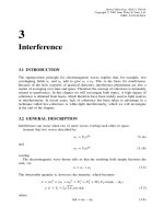
however, the same locations in the two cases. A time-average recording of a vibrating
turbine blade therefore looks like that shown in Figure 12.2(a) when applying ordinary
holography, and that in Figure 12.2(b) when applying TV holography. We see that the

main difference in the two fringe patterns is the speckled appearance of the TV holography
picture.
When applied to static deformations, the video store in Figure 12.1 must be included.
This could be a video tape or disc, or most commonly, a frame grabber (see Section 10.2)
in which case the video signal is digitized by an analogue-to-digital converter. Assume
that the wave scattered from the object in its initial state at a point on the TV target is
described by
u
1
= U
o
e
iφ
o
(12.9)
After deformation, this wave is changed to
u
2
= U
o
e
i(φ
o
+2kd)
(12.10)
300
COMPUTERIZED OPTICAL PROCESSES
Holography ESPI
(a) (b)
Figure 12.2 (a) Ordinary holographic and (b) TV-holographic recording of a vibrating turbine

blade. (Reproduced by permission of Prof. O. J. Løkberg, Norwegian Institute of Technology,
Trondheim)
where d is the out of plane displacement and where we have assumed equal field ampli-
tudes in the two cases. Before deformation, the intensity distribution on the TV target is
given by
I
1
= U
2
+ U
2
o
+ 2UU
o
cos(φ − φ
o
)(12.11)
where U and φ are the amplitude and phase of the reference wave. This distribution is con-
verted into a corresponding video signal and stored in the memory. After the deformation,
the intensity and corresponding video signal is given by
I
2
= U
2
+ U
2
o
+ 2UU
o
cos(φ − φ

0
− 2kd) (12.12)
These two signals are then subtracted in real time and rectified, resulting in an intensity
distribution on the monitor proportional to
I
1
− I
2
= 2UU
0
|[cos(φ − φ
0
) − cos(φ − φ
0
− 2kd)]|
= 4UU
0
| sin(φ − φ
0
− kd)sin(kd)| (12.13)
The difference signal is also high-pass filtered, removing any unwanted background signal
due to slow spatial variations in the reference wave. Apart from the speckle pattern due to
the random phase fluctuations φ − φ
0
between the object and reference fields, this gives
the same fringe patters as when using ordinary holography to static deformations. The
dark and bright fringes are, however, interchanged, for example the zero-order dark fringe
corresponds to zero displacement.
This TV holography system has a lot of advantages. In the first place, the cumbersome,
time-consuming development process of the hologram is omitted. The exposure time is

quite short (
1
25
s), relaxing the stability requirements, and one gets a new hologram
each
1
25
s. Among other things, this means that an unsuccessful recording does not have
the same serious consequences and the set-up can be optimized very quickly. A lot of
DIGITAL HOLOGRAPHY
301
loading conditions can be examined during a relatively short time period. Time-average
recordings of vibrating objects at different excitation levels and different frequencies are
easily performed.
The interferograms can be photographed directly from the monitor screen or recorded
on video tape for later analysis and documentation. TV holography is extremely useful for
applications of the reference wave modulation and stroboscopic holography techniques
mentioned in Section 6.9. In this way, vibration amplitudes down to a couple of angstroms
have been measured. The method has been applied to a lot of different objects varying
from the human ear drum (Løkberg et al. 1979) to car bodies (Malmo and Vikhagen 1988).
When analysing static deformations, the real-time feature of TV holography makes it
possible to compensate for rigid-body movements by tilting mirrors in the illumination
beam path until a minimum number of fringes appear on the monitor.
12.3 DIGITAL HOLOGRAPHY
In ESPI the object was imaged onto the target of the electronic camera and the interference
fringes could be displayed on a monitor. We will now see how the image of the object
can be reconstructed digitally when the unfocused interference (between the object and
reference waves) field is exposed to the camera target. The experimental set-up is therefore
quite similar to standard holography.
The geometry for the description of digital holography is shown in Figure 12.3. We

assume the field amplitude u
o
(x, y) of the object to be existing in the xy-plane. Let the
hologram (the camera target) be in the ξη-plane a distance d from the object. Assume
that a hologram given in the usual way as (cf. Equation (6.1))
I(ξ,η) =|r|
2
+|u
o
|
2
+ ru
∗
o
+ r
∗
u
o
(12.14)
is recorded and stored by the electronic camera. Here u
o
and r are the object and reference
waves respectively. In standard holography the hologram is reconstructed by illuminating
the hologram with the reconstruction wave r. This can of course not be done here. How-
ever, we can simulate r(ξ,η) in the ξη-plane by means of the computer and therefore also
construct the product I(ξ,η)r(ξ,η). In Chapter 4 we learned that if the field amplitude
distribution over a plane is given, then the field amplitude propagated to another point
Hologram ImageObject
y
y

′
x
′
d
′
d
x
h
x
Figure 12.3