Câu hỏi GIS, viễn thám, mô hình toán
Bạn đang xem bản rút gọn của tài liệu. Xem và tải ngay bản đầy đủ của tài liệu tại đây (744.73 KB, 10 trang )
<span class='text_page_counter'>(1)</span><div class='page_container' data-page=1>
RUSLE and SDR Model Based Sediment Yield Assessment in a GIS and
Remote Sensing Environment; A Case Study of Koga Watershed, Upper
Blue Nile Basin, Ethiopia
<b>Habtamu Sewnet Gelagay</b>
<i>Information Network Security Agency, Spatial Data Infrastructure, Addis Ababa, Ethiopia</i>
*<b><sub>Corresponding author:</sub></b><sub> Gelagay HS, Geospatial Data Analyst, Spatial Data Infrastructure Program, Information Network Security Agency, Spatial Data Infrastructure,</sub>
Addis Ababa, Ethiopia, Tel: 251918020778; E-mail:
<b>Rec date: </b>Feb 29, 2016;<b>Acc date: </b>Apr 14, 2016;<b> Pub date: </b>Apr 24, 2016
<b>Copyright:</b>© 2016 Gelagay HS. This is an open-access article distributed under the terms of the Creative Commons Attribution License, which permits unrestricted use,
distribution, and reproduction in any medium, provided the original author and source are credited.
<b>Abstract</b>
Soil erosion and the subsequent sedimentation are the major watershed problems in Ethiopia. Removal of top
fertile soil, siltation of Koga irrigation reservoir, clogging of irrigation canal by sediment and reduction of irrigated land
are the major threat of Koga watershed. Hence, this study was attempted to assess and map the spatial distribution
of sediment yield of Koga watershed in a GIS and remote sensing environment. Sediment yield is dependent on
factors of soil erosion such as rainfall erosivity, soil erodibilty, land use land cover (C and P) and topography (LS)
and sediment delivery ratio of the drainage basin to the total amount of sediment yield by sheet and channel
erosion. RUSLE framed with GIS and Remote sensing technique was therefore employed to assess the amount of
soil loss existed in KW. Main stream channel slope based sediment delivery ratio analysis was also carried out. Soil
map (1:250,000), Aster DEM (30 × 30 m), Thematic Mapper (TM) image (30 m × 30 m) of the year 2013, thirteen
years (2000-2013) rainfall records from four rain gauge stations and topographic map (1:50,000) were the major
data used. The estimated mean annual SY delivered to the out let of KW was found to be 25 t ha-1<sub>year</sub>-1<sub>. Most</sub>
critical sediment source areas are situated in the steepest upper part of the watershed due to very high computed
soil loss and sediment delivery ratio in this part. It could be therefore difficult to attain the intended goal of Koga
irrigation reservoir positioned at lower part of the watershed. Sustainable land management practices have to be
conducted in the upper part of the watershed by taking each stream order as a management unit to increase the
storage capacity, and/or lessen the transportation capacity of the watershed. Proper drainage construction and
stream bank stabilization via vegetative cover have to widely implement to safely dispose the eroded sediment.
<b>Keywords: </b>Sediment yield; RUSLE; SDR; Watershed management;
Koga watershed; Ethiopia
<b>Introduction</b>
Soil erosion and the consequent sedimentation are the major
watershed problems in many developing countries like Ethiopia [1].
Soil erosion and sediment yield from catchments are therefore key
limitations to achieving sustainable land use and maintaining water
quality in streams, lakes and other water bodies [2]. Eroded material
derived from the watershed, riverbed and banks transported with the
flow as sediment transport, either in suspension or as bed load.
Ultimately, this sediment redeposit and often causing problems in
downstream areas. On the other hand, the sediment load passing the
outlet of a catchment forms its sediment yield. Sediment yield can be
emanated from point source discharge (mining and construction
process) and non-point sources (run off from agricultural land and
bank erosion) [3]. Sediment load is reliant on factors of soil loss and
sediment delivery ratio [4].
Many of Ethiopia’s hydroelectric power and irrigation reservoirs
such as Aba-Samuel, Koka, Angerib, Melka Wonka, Borkena, Adarko
and Legedadi has been threatened by the heavy sedimentation. Thus,
these dams have been suffered from reduction in their capacity and life
span, quality of water and require costly operation for removal and
operation and thus these dams loss their intended services [4,5].
Hydrosult Inc. et al. [6] found the Ethiopian Plateau as the main
source of the sediment in the Blue Nile system. FAO [7] estimated 10%
sediment delivery rate to the rivers in Abay basin. It implies that 90%
of sediment remains in the land scape. This estimate is lower than 30%
estimated by Hurni [8]. FAO [7] also gives a range of soil erosion from
2.3 tha-1<sub>year</sub>-1<sub> to 212.9 tha</sub>-1<sub>year</sub>-1<sub> and a sediment load of 19.46 t</sub>
ha-1<sub>year</sub>-1<sub> which translates into 195 t ha</sub>-1<sub>year</sub>-1<sub> of erosion for the basin</sub>
as a whole. This estimate of sediment yield is quite close to 23.5 t
ha-1<sub>year</sub>-1<sub> estimated by Kefenie [9] at Ajenie-Gojjam.</sub>
Awulachew et al. [1] reviewed that sediment transport and
sedimentation are critical problems in the Blue Nile Basin. The
socioeconomic development in the basin particularly in downstream
areas is hampered by sediment deposition. For instances, Gilgel Gibie I
hydroelectric power reservoir situated in Blue Nile basin has been
threatened by sedimentation, hence it loss it’s intended services [4].
Sediment yield to the stream network also poses numerous socio
economic effects such as damage of recreational value of water;
decreased value of water for domestic, industrial, or waste disposal
function; interruptions in stream flow characteristics resulting in
downstream flooding and decreased storage. In addition, excessive
sedimentation clogs stream and irrigation channels and increases costs
for maintaining water conveyances and have a variety of negative
effects on downstream agriculture and fisheries as well as on peoples'
nutritional well-being [10,11].
</div>
<span class='text_page_counter'>(2)</span><div class='page_container' data-page=2>
consequence of high sediment loads [1]. Siltation of water body caused
by sedimentation reduces sunlight penetration and affecting water
temperature, reduces photo synthesis and as a result the survival of
submerged aquatic vegetation, degrades the fish habitat (muddy water
fouls the gills of the fish) and upset the aquatic food chain.
Sedimentation also causes eutrophication (excessive plant growth) due
to excessive load of nutrients such as nitrogen and phosphorus and it’s
deposition at higher level creates an increased level of non-living
periphyton or otherwise degrades water quality [3,12]. This problem
has been recorded in Blue Nile basin particularly at Gilgel Gibie I
[13,14].
Koga watershed (KW), with its outlet to small dam (Koga irrigation
and fishery dam) is threatened by the above problems. Ministry of
Natural Resources and Environmental Protection stipulated that the
rate of soil loss in the furthest upstream portions of the watershed
exceeds the soil formation rate [15]. Similarly, loss of top fertile soil,
sedimentation or siltation of reservoir (Koga irrigation and Fish dam),
clogging of irrigation channels, reduction of irrigated area and
decreases in crop productivity due to reduction in the quality as well as
quantity of irrigation water are the major problems in KW [16]. The
extension of these problems will particularly threaten Koga irrigation
reservoir in particular and jeopardize the farmers’ agricultural
production and productivity of the irrigable land in the watershed.
This problem may make the people in the watershed to be food in
secured. Furthermore, the life supporting system may be worsened and
ultimately reach in an irremediable condition. The generated sediment
yield from the catchment could also affect the ecosystem of Lake Tana.
The quantification of spatially distributed sediment yield and
precise identification of sediment source and erosion vulnerable areas
is noteworthy for watershed conservation prioritization and for
reduction of the socio-economic and environmental cost posed by
sedimentation on various irrigation and hydropower reservoirs,
channels and conservation areas as stated by Tenaw and Awulachew
[17]. Sediment yield information is therefore a critical factor in
identifying non-point source pollution, comprehensive control of small
and medium sized watershed as well as in the design and maintenance
of the construction of hydro structures such as dams and reservoirs.
The knowledge of the quantitative and spatial distribution of soil
erosion and sedimentation is thus required to Control the sediment
load and has important implication for the study of offsite
environmental impact due to exported sedimentation and onsite
erosion control.
Various previous studies have been conducted in Koga irrigation
and watershed management project specifically to know the potential
loss of capacity in the Koga reservoir due to sedimentation over the
design life of the project by employing different bathy metric survey
and empirical and mathematical sediment estimation method. But,
those studies did not consider the spatial patterns of sediment yield
and sediment delivery ratio of the Koga watershed and any one of the
previous study were not simulate sediment yield using GIS and remote
sensing techniques with geospatial processing capabilities. Besides,
Chalachew [18] recommends further detail empirical sediment yield
estimation because of the discrepancy between the measured and
simulated volume of sediment in Koga reservoir. Likewise, Nigusie and
Yared [19] recommend advanced studies to monitor siltation rate in
the watershed. Therefore this study was attempted to assess and map
the spatial distribution of sediment yield using Sediment deliver ratio
(SDR) and Revised Universal Soil Loss Equation (RUSLE) of Koga
watershed in a GIS and remote sensing environment. Specifically, an
effort was made to map and assess the sediment delivery ratio and soil
loss of Koga watershed and to identify sediment hotspot areas for
conservation prioritization.
<b>Research Methods</b>
<b>Study area description</b>
The geographic location of the Koga watershed extends from
11.16N to 11.41N Latitude and 37.03° E to 37.28° E longitude. A total
area of the watershed is about 28,000 hectare (Figure 1). Topography of
the area exhibits distinct variation and contains flat low-laying plains
(0% slope) surrounded by steep hills (70% slopes) and rugged land
features. Thus, Koga catchment can be divided in to a narrow steep
upper catchment draining the flanks of Mount Adama range and the
remainder on relatively flat plateau sloping gently west wards. The
altitude ranges from 1885 to 3131 m.a.s.l. The nature of the
topographical features has made the area very liable to heavy gully
formation and extensive soil erosion. The Koga River is a tributary of
the Gilgel Abay River in the head water of the Blue Nile catchment.
The Gilgel Abay flows in to Lake Tana. The river is 64 km long flowing
into Gilgel Abay River. Koga irrigation and fish reservoir is located in
the north western confluence point of the watershed. Its mean annual
precipitation is 1628.2 mm with a maximum and minimum mean
annual temperature between 17.10C and 28.4C. The area experiences
the main rainy season ‘me her’ which commences in June and extends
to September. There are about seventeen (18) kebeles (smaller
administrative unite) in the watershed. The total population of the
watershed excluding the local capital Merawi town was estimated to be
around 57,155 (33475 male and 23627 female) [20]. Majority of the
population is engaged in agriculture. Koga large scale irrigation and
watershed development project is implemented within this watershed
territory since 2009. The Koga Irrigation and Watershed Development
Project cover about 7,000 ha of irrigable land and 22,000 ha of land
watershed management in the upstream part of the watershed. Only
1,000 ha of the irrigation command area are located within the
catchment territory. The remaining 6,000 ha are irrigation command
area outside of the watershed boundary to the North direction.
Figure 1: Study area map.
<b>Sources and techniques of data collection</b>
</div>
<span class='text_page_counter'>(3)</span><div class='page_container' data-page=3>
lower catchment based on their relative location; primary data such as
ground control points (GCPs) were collected using global positioning
system (GPS) in each strata of the watershed for each major land use
or land cover types to train the image using supervised image
classification and to produce thematic land use land cover map.
Ground control points (GCPs) for each major land use/cover types
were also collected for accuracy validation. Intensive field observation
were concurrently conducted to assess the state of the watershed and to
identify where and what kind of support practice had been constructed
in the watershed (Figure 2).
Likewise, secondary data such as the soil map (1:250,000) obtained
from Nile river basin master plan, Aster Digital Elevation Model (30 m
× 30 m) downloaded from Global land cover facility
(www.landcover.org) which was resampled to 20 × 20 meter spatial
resolution, Thematic Mapper (TM) multi spectral image with spatial
resolution of 30 meter of the year 2013 down loaded from global land
cover facility topographic map (1:50,000) taken from Bureau of
Agriculture and thirteen years (2000-2013) rainfall records from four
rain gauge stations (Merawi, Meshenti and Bahir Dar and Durbetie)
obtained from National Meteorological Agency were used to estimate
the mean annual soil loss, sediment delivery ratio (SDR) and sediment
yield of KW. The Google earth image was also used to digitize and
produce water body (Koga reservoir) map of the study area. Other
published and unpublished materials such as research reports, census
reports and journal obtained from different sources were also
employed.
Figure 2: Mean monthly Rainfall and Temperature of KW.
<b>Method of data analysis</b>
RUSLE parameterization: Revised Universal Soil Loss Equation
(RUSLE), which is an empirical model developed by Renard et al. [21],
framed with GIS and remote sensing techniques were employed to
compute the mean annual soil loss of KW. Laflen and Molden [22]
inveterate the possible application of RUSLE on every continent on
earth where soil loss by water is a problem. Therefore examined the
application of the RUSLE in the Ethiopian highlands (Tigray Region)
after Hurni effort to adopt USLE [23]. Flow convergence and
divergence in a complex terrain were not considered by RUSLE in this
study; however it can be applied in many circumstances even on steep
and undulating terrain. A gain it was conducted at regional scale,
hence didn’t consider the spatial variability of soil loss process at
catchment or watershed level. The study by Zhang et al. [24] and Van
Remortel et al. [25] confirmed the limitation of the USLE and RUSLE
method of soil loss estimation at regional scale in considering the
spatial dynamics of soil loss process and in extracting slope length and
gradient (LS) factor. Thus, here in this paper, RUSLE was employed at
intermediate watershed or catchment level by incorporating the
advanced LS factor computation approach. RUSLE is empirically
expressed as:
SE (metric tons ha-1<sub>year</sub>-1<sub>)=R*K*LS*C*P (1),</sub>
Where SE is the mean annual soil loss (metric tons ha-1<sub>year</sub>-1<sub>); R is</sub>
the rain fall erosivity factor [MJ mm h-1<sub> ha </sub>-1<sub> year</sub>-1<sub>]; K is the soil</sub>
erodibility factor [metric tons ha-1<sub>MJ</sub>-1<sub>mm</sub>-1<sub>]; LS is the slope </sub>
length-steepness factor (dimensionless); C is the cover and management
factor (dimensionless, ranges from zero to one); and P is the erosion
support practice or land management factor (dimensionless and ranges
from zero to one). This model was simulated by GIS and remote
sensing techniques as shown in the Figure 3 below.
Figure 3: Conceptual Frame work of Soil Loss.
As in Figure 3, once all the RUSLE parameter had been surveyed
and calculated, each raster layer of the RUSLE parameter was
discretized to a resampled DEM grid size of 20 m × 20 m resolution.
The layers were then multiplied pixel by pixel using Equation one and
raster calculator geoprocessing tool in Arc GIS 10.1 environment to
compute and map the spatial pattern of the mean annuals soil loss in
KW.
Rainfall erosivity (R) factor: The rainfall erosivity (R) factor
</div>
<span class='text_page_counter'>(4)</span><div class='page_container' data-page=4>
Ethiopian condition is based on the available mean annual rainfall data
and the equation is expressed as;
R=-8.12+(0.562 × P) (2),
where R is rain fall erosivity factor and P is the available mean
annual rain fall data.
Inverse distance weighted (IDW) method was employed to produce
uninterrupted rain fall data from point mean annual rain fall data
obtained from four rainfall station for each grid cell in Arc GIS10.1
environment. From this continuous rainfall data, the R-value of each
grid cell was calculated using Equation (2) and raster calculator
geo-processing tool (Table 1).
<b>No</b> <b>Station<sub>Name</sub></b>
<b>Location</b> <b>Altitude</b>
<b>Mean Annual</b>
<b>Rain fall (mm)</b>
Latitude (Y) Longitude (X)
1 Bahir Dar 11.59 37.388 1800 1371.743
2 Merawi 37.164 2000 2000 1570.87
3 Meshenti 11.5 37.3 1969 1287.74
4 Durbetie 11.359 36.956 1984 1696.74
Table 1: Rain Gauge Stations around the Study Area.
Soil erodibility (K) factor: Soil erodibility is the manifestation of the
inherent resistance of soil particles for the detaching and transporting
power of rain fall [29]. The K-factor is empirically determined for a
particular soil type and reflects the physical and chemical properties of
the soil, which contribute to its erodibility potential [30]. Hurni and
Hellden [23,28] recommended the K values based on easily observable
soil color as an indicator for the erodibility of the soil in the highlands
of Ethiopia. Thus, the soil map of KW was clipped from soil map
(1:250,000) of the Blue Nile river master plan and the soil type of the
watershed were classified based on their color as recommended by
Hurni and Hellden to assign the K-value [23,28]. The water body
(Koga reservoir) map of the study area was clipped from google earth
image and assigned the K-value based on Erdogan et al. [31]
recommendation. Koga soil map was then dissolved with Koga
reservoir map clipped from Google earth image. Finally, once the
vector to raster conversion of soil map of the study area was done, the
grid format was reclassified into K-factor value for each soil class in
Arc GIS 10.1 using reclassification geo processing tools.
Slope length-steepness (LS) factor:The (LS) factor is the ratio of soil
loss per unit area from afield slopes to that from a 22.13 m length of
uniform 9 percent slope under otherwise identical conditions [29].
Slope length (L sub factor) in this case represents the distance between
the source and culmination of inter rill process. The culmination is
either the point where slope decreases and the resultant depositional
process begins or the point where concentration of flow into rill or
other constructed channel such as a terrace or diversion [21,29].
In RUSLE, the three dimensional complex nature of terrain was not
considered in the computation of slope length topographic sub-factor
rather soil loss was tied with only with slope length [32]. However,
other researchers claimed that soil loss does not depend on slope
length for three dimensional complex terrains where there is flow
convergence and divergence. For instance, Zhang et al. [24] condemn
the USLE and RUSLE method of slope length-steepness (LS) factor
calculation and develop advanced LS-tools algorithms which fill the
puzzles of the USLE and (R)USLE method, even though the algorithm
is not presently supported in Arc GIS10.1 environment. Hickey [33]
also postulated that the limitation of slope length computation in
USLE can be resolved by using the cumulative uphill length from each
cell which accounts for convergent flow paths and depositional area.
Similarly, studies by Desmet and Govers [34]; Moore and Burch
[35,36]; Mitas and Mitasova [37]; and Simms et al. [38] indicated that
slope length should be substituted by upslope contributing area. Thus,
it is helpful to consider the three dimensional complex terrain
geometry as well the upslope contributing area to better comprehend
the spatial distribution of soil erosion and deposition process. This
study was therefore employed the following advanced LS factor
computation method based on up slope contributing area suggested by
Desmet and Govers [34]; Moore and Burch [35,36]; Mitasova and
Mitas [39]; and Simms et al. [38].
LS=(As/22.13)0.6(sin B/0.0896)1.3………(3)
Where LS is slope steepness-length factor, As is specific catchment
area, i.e., the upslope contributing area per unit width of contour
drains to a specific point (flow accumulation × cell size) and B is the
slope angel. LS-factor was computed in Arc GIS raster calculator using
the map algebra expression in equation (4) below suggested by
Mitasova and Mitas [39]; and Simms et al. [38].
POW ([flow accumulation]×cell size/22.13, 0.6)×POW (sin ([slope]
×0.01745)/0.0896, 1.3)….(4)
This study was therefore used the above modified and advanced
approach of determining slope length and gradient (LS) factor. The
values of S were directly derived from 20 meter resolution DEM.
Similarly, flow accumulation was derived from the DEM after
conducting Fill and Flow Direction processes in Arc GIS 10.1 in line
with Arc Hydro tool. Flaw accumulation grid represents number of
grid cells that are contributing for down ward flow and cell size
represents 20 m × 20 m contributing area.
Cover and management (C) factor: It represents the ratio of soil loss
from land with specific vegetation to the corresponding soil loss from
continuous fallow [10,29]. Cover and management (C) factor is the
solely factor that easily changed overtime in most cases and it regarded
mostly in developing conservation strategy. Unsupervised
classification was directed to identify the major land use land cover
types in the watershed. Based on the information obtained from
unsupervised classification, supervised classification by the help of
ground control (training) points was conducted to produce thematic
land cover maps of the study area. Ground control points (GCPs)
collected using hand held GPs were also employed to validate the
accuracy of thematic land use land cover classification process. Land
use land cover raster map of KW was then converted to vector format
to assign the corresponding cover and management (C) factor value
obtained from different studies.
Support practice (P) factor:Support practice (P) factor is the ratio of
soil loss with a specific support practice to the corresponding loss with
up and down slope cultivation [29]. This factor considers the erosion
control practices such as contouring, strip cropping and terracing
which reduces the eroding power of rainfall and runoff by their impact
on drainage patterns, runoff concentration and runoff velocity [40].
</div>
<span class='text_page_counter'>(5)</span><div class='page_container' data-page=5>
computed the P-value by categorizing the land in to agricultural land
and other land major kind of land use types (Table 2). Finally, they
sub-divided the agricultural land (cultivated land) in to six slope
classes and assigned p-value for each respective slope class as many
management activities are highly dependent on slope of the area. In
this study, this method of combining general land use type and slope
was therefore adopted. Values for this factor were therefore assigned
considering local management practices along with values suggested in
Wischmeier and Smith [29].
<b>Land use type</b> <b>Slope (%)</b> <b>P-factor</b>
Agricultural land (cultivated land)
0-5 0.1
5-10 0.12
1-10 0.14
20-30 0.19
30-50 0.25
50-100 0.33
Other land All 1
Table 2: P-Value [29].
Water body, grazing, shrub and forest lands were therefore referred
as other land and given the P-value regardless of the slope class they
have but cultivated land of the watershed was categorized into six slope
class and given P-values as discoursed by Wischmeier and Smith [29].
Lastly, the classified land use land cover and slope thematic map has
been converted in to vector format and the corresponding P values
were assigned to the combination of each land use land cover and slope
classes.
Sediment Delivery Ratio (SDR) estimation: Sediment Delivery Ratio
(SDR) is a fraction of gross erosion that is transported from a given
area in a given time interval. It is a measure of sediment transport
efficiency which accounts for the amount of sediment that is actually
transported from the eroding sources to a catchment outlet compared
to the total amount of soil that is detached over the same area above
that point.
The sediment delivery ratio value in a given watershed indicates the
integrated capability of a catchment for storing and transporting the
eroded soil. It compensates for areas of sediment deposition that
become increasingly important with increasing catchment area and
therefore, determines the relative significance of sediment sources and
their delivery [41]. It is affected by many highly variable physical
characteristics of a watershed such as drainage area, slope, relief-length
ratio, runoff-rainfall factors, land use land cover and sediment particle
size [2]. The amount of floodplain sedimentation occurring and the
presence of hydrologically controlled areas such as ponds, reservoirs,
lakes and wetlands also affect the rate of sediment delivery to the
watershed mouth.
Numerous Sediment Delivery Ratio (SDR) relationships have been
developed based on combinations of the variable physical
characteristics of a watershed [42]; but, their application is limited to
only small catchments with adequate data [2]. Williams and Berndt
[43] found that the average stream channel slope is more significant
than other parameters in estimating sediment delivery ratio, which is
expressed as a function of percent slope of main stream channel.
Empirically, Sediment Delivery Ratio in this case is expressed as;
SDR = 0.627 × (SLP) 0.403………
(5),
Where, SLP is percent slope of main stream channel. Onyando et al.
[44] confirmed that Williams and Berndt [43] method of main stream
channel slope gradient based sediment delivery ratio estimation
provides reasonable result in a case of in adequate data. This empirical
equation was therefore used in this intermediate watershed (Koga
watershed) where there is no adequate data as illustrated in the
following diagram (Figure 4).
Figure 4: Diagram of Sediment Delivery Ratio Analysis.
Digital Elevation Model (DEM) was corrected for sink as well grids
of flow direction, flow accumulation and stream network were
determined. After conducting terrain preprocessing, the flow path was
generated using Arc GIS extension of HEc GeoHMS 10.1. By taking
the flow path and raw DEM, the average mainstream channel slope
(SLP) values in percentage for each cell in the flow path was computed
for the estimation of the SDR value for that cell amount upstream from
that cell as indicated in the above diagram. Each cell in the flow path
can be considered as the outlet of its upstream catchment. Therefore,
the SDR value of that cell measures the sediment delivery capacity of
its upstream catchment as stated by Li et al. [45].
</div>
<span class='text_page_counter'>(6)</span><div class='page_container' data-page=6>
measurement in watershed lacking adequate sediment regime like
Koga watershed as stated by Benedict and Andreas [2]; accurate
estimation of sediment delivery ratio is an important and effective
approach. Therefore, for this study sediment yield was computed by
superimposing the raster layer of mean annual soil loss obtained by
RUSLE model analysis and the channel slope based sediment delivery
ratio using equation (6).
Sy =
∑
�= 1
�
��� � �� (6)
Where n is the total number of cells over the catchment, SE is the
amount of soil erosion produced within the ith<sub> cell of the catchment</sub>
estimated using Equation (1) and SDR is the fraction of SE that
ultimately reaches the nearest channel computed by. In a GIS
framework, the raster layer of sediment yield for the watershed (SY)
was estimated by overlaying the raster layer of mean annual soil loss
and sediment delivery ratio using raster calculator geo-processing tools
(Figure 5).
Figure 5: Diagram of Sediment Yield Estimation.
<b>Result and Discussion</b>
<b>RUSLE based soil loss valuation</b>
Rainfall Erosivity (R) factor: Rain fall erosivity (R) value ranges
from 715 (in the outlet part) to 945 (inlet part) were estimated using
equation (2) and raster calculator geo-processing tool. The R-value of
874 at Merawie station (nearest station to watershed) has great weight
to the R-value of the watershed. Thus, the R-value in most part of the
watershed was found to be 874 except a little variation at the lower and
north western part of the watershed. This implies that the influence of
rain fall erosivity is nearly similar in the study area with a little
exception at the lower and north western part of the watershed.
Soil Erodibility (K) factor: Eutric Vertisols (Black), Eutric Regosols
and Haplic Luvisols (Brown), Haplic Nitosols and Ali sols (Red) soil
classes were identified and given the K-value of 0.15, 0.2 and 0.25 for
Black, Brown and Red soil color respectively based on Hurni and
Hellden soil color based K-value recommendation [23,28]. The
K-value of zero [31] was assigned for water body (Koga reservoir). Haplic
Nitosols and Ali sols (0.25), which are highly susceptible for the
eroding power of rain fall, are dominant in the upper part of the
watershed; as a result this part could be seriously affected by soil loss
by water. On the other hand, the lower and middle part of the
watershed are dominated by less erodible (Vertisols) and moderately
erodible (Regosols and Luvisols) soil class, hence this part could have
minimal soil loss contribution.
Slope length-steepness (LS) factor:The slope length-steepness (LS)
value ranges from 0 (flatter lower and middle part) to 109 (steepest
upper part) was estimated using the map algebra expression (equation
4) in raster calculator Arc GIS geo-processing tools. The topographic
(LS) factor of RUSLE has therefore significantinfluence in the upper
part of the watershed and vice versa in the lower and middle part.
Cover and management (C) factor:The C-factor value taken from
different studies were given for the major land use land cover types of
the study area identified by supervised image classification in ERDAS
imagine 10 environments (Table 3).
<b>Land use land cover type C-factor value</b> <b>References</b>
Water body 0 Erdogan et al. [31]
Cultivated land 0.1 Hurni [8,25]
Forest land 0.01 Hurni [8,25]
Shrub land 0.014 Wieshmier and Smith [29]
Grazing land 0.05 Hurni [8,25]
Table 3: C-Factor value of the watershed adopted from different
studies.
Maize and millet are the major crops cultivated in most of the
middle and lower part of the watershed with the cover and
management factor value of 0. The soil loss in the middle and lower
part of the watershed could be therefore high due to the predominance
of cultivated land (maize and Millet).
</div>
<span class='text_page_counter'>(7)</span><div class='page_container' data-page=7>
Finally, each layers of RUSLE parameter was organized in a grid
format with a cell size of 20 m × 20 m and the soil loss map of the
watershed was produced (Figure 6). The computed mean annual soil
loss of the study area was therefore found to be 47.4 ton ha-1<sub>year</sub>-1<sub> with</sub>
a range of 0 (lower par, specifically at Koga reservoir) to 265 ton
ha-1<sub>year</sub>-1<sub>. On annual bases, the total soil loss of the watershed was</sub>
found to be 255283 tones. Topographic (LS) and soil erodibility (K)
factors were found to be the major soil loss parameter.
Figure 6: Soil Loss Rate Map.
<b>Sediment delivery ratio (SDR) assessment</b>
Spatially distributed Sediment Delivery Ratio (SDR) map was
produced by computing the average channel slope value in percent for
each cell in the flow path using HEc GeoHMS 10.1 in a GIS
environment (Figure 7). Hence, as shown in Figure 7 (left) below, main
stream channel slope of Koga watershed ranges from 0.0007 (the lower
catchment) to 0.08 percent (steepest upper catchment).
Figure 7: Stream Channel Slope (left) and Sediment Delivery Ratio
(right) Map.
Figure 8: Main stream Channel Slope Profile.
Lastly, the Sediment Delivery Ratio (SDR) values range from 0.04 to
0.3 was computed using raster calculator geo processing tools and
Equation (3) in ArcGIS10.1 environment. This implies that in Koga
watershed (KW), the eroded materials which passes to the channel
system and contributes to sediment yield ranges from 4.4 to 30
percent. In the steeper, narrower and upper part of the watershed, 30
percent of the eroded soil particles passes to the channel system and
delivered to Koga watershed (KW) out let. It is therefore, this part of
the watershed has high capability to transport the eroded material, but
less storage capacity. Whereas, in the wider, flatter and lower part of
the watershed only 4 percent of the gross soil loss is delivered to the
outlet of Koga watershed (KW). It does mean that 96 percent of the
eroded materials are redeposited in the catchment of the watershed.
Hence, this part of the watershed has excellent storage capacity of the
eroded soil, but streams in this part have less sediment delivery
capacity.
As point up in the Figure 7 (right) and Table 4, first order streams
with very high sediment delivery capacity (> 0.2) are situated in
stepper and narrower parts of the upper catchment. In this part, 24.9
per cent of the eroded soil particles could be transported to the out let
of Koga watershed (KW) annually. While, the second most critical
sediment delivery class (0.15-0.2) are located in the gentle slope lower
parts of the watershed. Fortunately, some of these second vital areas are
found in the lower parts of Koga irrigation reservoir but not all. These
</div>
<span class='text_page_counter'>(8)</span><div class='page_container' data-page=8>
<b>Numeric SDR (Sediment Delivery Ratio class)</b> <b>Sediment delivery capacity class</b> <b>Mean SDR capacity (%)</b>
0.044-0.1 low 7.2
0.1-0.15 moderate 12.5
0.15-0.2 high 17.5
>0.2 Very high 24.85
Table 4: Numeric SDR Class and Contribution to Sediment Yield.
On average, the sediment delivery capacity of KW is about 0.17.
This indicates that a mean of 17% of the eroded soil materials (soil,
nutrient and other pollutant) could be delivered to Koga watershed
(KW) outlet and 82.5% of the eroded soil materials are redeposit in the
catchment of the watershed. But, FAO [7] estimated 10% sediment
delivery rate to the rivers in Abay basin where this study area belongs
to.
Ouyang and Bartholic [42] point out that watersheds with steep
slopes, smaller drainage area and the fields with short distance to the
streams have a higher sediment delivery ratio than a watersheds with
flat and wide valleys, large drainage area and fields with long distance
to streams. In the same way, the result of this study from the above
map showed that the SDR values in the steeper, fields with short
distance to stream and narrower upper catchment of the watershed
(upstream) are greater than those in flatter and wider middle and
lower catchment(near Koga reservoir) of the watershed. This is because
large areas have more chances to trap soil particles. Thus, the chance of
soil particles reaching the water channel system is low. Therefore, more
eroded soil in the upstream areas transported into the channels and
delivered out of the watershed. Ouyang and Bartholic [42] also
stipulated that the amount of floodplain sedimentation occurring and
the presence of hydro logically controlled areas such as ponds,
reservoirs, lakes and wetlands also affect the rate of sediment delivery
to the watershed mouth. Correspondingly, the sediment delivery ratio
values near Koga reservoir is quite smaller (7.2%). Besides the above,
the report of Merawi woreda office of agriculture confirmed that grass
strip development and alteration of the crop land into perennial fruit
tree and forage land has been done around Koga reservoir by Koga
watershed development project and the people jointly. Thus, reduction
in sediment delivery ratio near Koga reservoir could be due to these
vegetation cover increment in Koga reservoir buffer zones.
The SDR map was considered reasonable because it reflects that the
ultimate nature of sediment delivery that erosion occurs in the steeper
location will have more chances to be transported into the channels
than to be deposited down slope.
<b>Sediment yield estimation</b>
Sediment yield was quantified using the channel slope based SDR
model [43], expressed as the percent of annual soil erosion by water
estimated by RUSLE that is delivered to a particular point in the
drainage system. As a result, the mean annual soil loss in Koga
watershed was estimated in the above section (3.1) and found to be
47.4 t ha-1 year-1. Likewise, the sediment delivery ratio was estimated
and discussed in chapter (3.2) by taking main stream channel slope as
a main parameter and on average the sediment delivery rate of 17.05
percent was estimated in Koga watershed. Thus, spatially distributed
map of sediment yield was produced through cell by cell multiplication
of the raster layer of sediment delivery ratio (SDR) and mean annual
soil loss in Arc GIS10.1 environment (Figure 8).
Figure 9: Sediment Loss (SE), Sediment Delivery Ratio (SDR) and
Sediment Yield (SY) Map.
Recall the above figure, the Sediment Yield (SY) of the watershed
ranges from 0 to 51 tone ha-1<sub>year</sub>-1<sub> which has a similar spatial pattern</sub>
with that of soil loss and sediment delivery ratio map. For the purpose
of identifying nonpoint source pollutants and the sediment load at the
end of the slope length, at the outlet of terrace diversion channels, or
sediment basins that are considered by RUSLE, the raster map of
sediment yield was classified into four sediment load class as illustrated
in Figure 9 and Table 5 below. Very high (>20 t ha-1<sub>year</sub>-1<sub>) and high</sub>
(10-20 t ha-1<sub>year</sub>-1<sub>) sediment load classes which accounts 23 and 8</sub>
</div>
<span class='text_page_counter'>(9)</span><div class='page_container' data-page=9>
and lower part of the watershed. This could be due to the presence of
hydrological controlled area (Koga irrigation reservoir) in the lower
part of the watershed. The presence of such hydrologically controlled
area could there for reduce the sediment delivery rate and thus the
sediment load as sediment load from the upper part of the watershed
could be enter in to the reservoir. Besides this, the reduction of
sediment yield in this part could also be due to the alteration of the
land use land cover from cultivation to protected forage land and
perennial crop land along with the development of grass strip around
the buffer zone of the reservoir for the past six years.
<b>Numeric range of SY (t</b>
<b>ha</b>-1<b><sub>year</sub></b>-1<b><sub>)</sub></b> <b><sub>ha</sub>Mean </b>-1<b><sub>year</sub></b>-1<b><sub>)</sub>SY </b> <b>(t</b> <b>Sediment load class</b> <b>Area (ha)</b> <b>Percent of total area</b> <b>Total annual SY</b> <b>% of total annual<sub>SY</sub></b>
0-5 2.5 Low 1172 90.4 2930 58.7
5-10 7.5 moderate 64 4.9 480 9.6
10-20 15 High 27 2.08 405 8.12
>20 35.5 Very high 33 2.54 1171.5 23.5
Table 5: Numeric Sediment Yield Range and Sediment Load Class.
Figure 9 and statistical Table 5 informed that, the total annual
sediment yield of Koga watershed was 4986 tone. The estimated mean
annual SY delivered to the out let of KW was found to be 25 t
ha-1<sub>year</sub>-1<sub> which is reasonable and realistic weigh against the </sub><sub>findings</sub>
of the previous studies. For case in point that the mean annual
sediment yield of 25 t ha-1<sub>year</sub>-1<sub> was measured in Anjeni-Gojjam</sub>
station by Kefeni [9]. FAO [7] also estimated a sediment load of 19 t
ha-1<sub>year</sub>-1<sub> for the Abbay river basin as a whole. But, is quite far from</sub>
140 kg ha-1<sub>year</sub>-1<sub> which is equivalent to 1.8 t ha</sub>-1<sub>year</sub>-1<sub> estimated by</sub>
Nigusie and Yared [19] using SWAT model.
<b>Conclusion</b>
Thefindings of this study demonstrate the simulation of sediment
yield in a GIS and remote sensing environment in areas where there is
no sufficient sediment regime like Koga watershed. It also shows how
the use of spatially capable technologies like remote sensing and GIS
helps in handling spatially dynamic data easily and efficiently. The
estimation of SY by integrating SDR and annual soil loss computed
from RUSLE could be replicated in other part of the upper Blue Nile
basin where sheet and rill erosion are dominant. Sediment yield
estimation in this study therefore plays a vital role for Koga large scale
irrigation reservoir in particular and for the watershed as a whole in
identifying non-point source pollution, critical sediment source areas
and to take site specific measures such as different drainage and water
harvesting structures. An accurate prediction of SDR is also important
in controlling sediments for sustainable natural resources development
and environmental protection.
Nature of the watershed (steepness, drainage area and distance to
stream), hydrologically controlled area (reservoir), land use land cover,
channel slope and soil factors were found to be determinant for
sediment yield assessment in Koga watershed.
Very high sediment load class was computed in the steeper upper
part of the watershed. It could be therefore disastrous due to the fact
that Koga irrigation and fishery reservoir which irrigate 7000 hectare is
positioned at the outlet of the watershed, thus the aforementioned
sediment load could cause siltation of the reservoir, clogging of
irrigation canal, even in reduction of the quality of irrigation water. It
is difficult therefore to attain the implied goal of Koga irrigation
reservoir. Siltation of the reservoir also could cause reduction in crop
productivity and finallyaffects the livelihood of the community who
depend on irrigation activities.
Hence, intensive sustainable soil and water conservation practices
should be carried out by taking each stream order as management unit
especially in the upper part where most critical sediment source areas
are situated. Each stream order should be treated uniquely and
conservation prioritization should be directed from first order streams
to highest order streams. In view of the fact that sedimentation could
affects Koga irrigation reservoirs and channel, proper drainage
construction and stream bank stabilization via vegetative cover have to
widely implemented. The report of Merawi office of agriculture and
field observation confirmed that soil and water conservation activities
were better implemented in the buffer zone of the reservoir irrespective
of watershed logic. But, conservation activities must be conducted
starting from the most upper catchment of the watershed by respecting
watershed logic and potential.
<b>References</b>
1. Awulachew SB, McCartney M, Steenhuis TS, Ahmed AA (2008) A review
of hydrology, sediment and water resource use in the Blue Nile Basin.
Colombo, Sri Lanka: International Water Management Institute.
2. Benedict MM, Andreas K (2006) Estimating Spatial Sediment Delivery
Ratio on large Rural Catchment. Journal of spatial hydrology 6: 1.
3. Klco B (2008) Effect of sediment loading on primary productivity and
Brachycerntridae survival in a third-order stream in Montana. BIO 35:
502-601.
4. Kebede W (2012) Watershed management: An option to sustain dams
and reserviours function in Ethiopia. Journal of environmental science
and technology 5: 262-273.
5. Adefemi OS, Olaofe O, Asaolu SS (2007) Seasonal variation in heavy
metal distribution in the sediment of major dams in ekiti-state. Pak J Nutr
6: 705-707.
6. Hydrosult Inc. Tecsult DHV (2006) Trans-Boundary Analysis: Abay-Blue
Nile Sub-basin. NBI-ENTRO (Nile Basin Initiative-Eastern Nile
Technical Regional Organization).
7. FAO (1986) Ethiopian Highlands Reclamation Study. 12 Rome.
8. Hurni H (1985) Erosion-productivity-conservation systems in Ethiopia.
In Proceedings of paper presented at the 4th international conference on
soil conservation, Maracay, Venezuela.
9. Kefeni K (1995) Soil Erosion and Conservation in Ethiopia. Paper
presented at the workshop on coffee and other crops in coffee growing
areas, Addis Ababa, Ethiopia.
</div>
<span class='text_page_counter'>(10)</span><div class='page_container' data-page=10>
11. BCEOM (2006) A bay River Basin Integrated development Master Plan
Project. Data Collection and Site investigation Survey and analysis on
Environment and Soil Conservation.
12. Brady NC, Weil RR (2002) The Nature and properties of Soil. 13th edn.
Prentice Hall, New Jersey, USA, p: 960.
13. Amare A (2005) Study of Sediment yield from the watershed of angereb
reservoir. Master’s Thesis, Department of Agricultural Engineering,
Alemaya University, Ethiopia.
14. Gessese A (2008) Prediction of sediment inflow for legedadie reservoir
(using SWAT watershed and CCHE1D sediment transport models).
Master’s Thesis, Faculty of Technology, Addis Ababa University, Ethiopia.
15. Ministry of Natural Resources and Environmental Protection, Water
Resource Development Authority (1995) Feasibility Study of Birr and
Koga Irrigation Project: Koga Catchment and Irrigation Study, Anex L,
Soil Conservation, Acres International Limited, Canada in Association
with Shawel Consult International, Ethiopia.
16. Gebreyohannis G, Taye SA, Bishop K (2009) Forest Cover and Stream
Flow in a Headwater of the Blue Nile: Complementing Observational
Data Analysis with Community Perception. Royal Swedish Academy of
Sciences.
17. Tenaw M, Awulachew BS (2009) Soil and Water Assessment Tool
(SWAT)- Based Runoff and Sediment Yield Modeling: A Case of the
Gumera Watershed in Lake Tana Sub basin. Intermediate Results
Dissemination Workshop on “Improved Water and Land Management in
the Ethiopian Highlands: Its Impact on Downstream Stakeholders
Dependent on the Blue Nile” IWMI Subregional Office for East Africa
and Nile Basin.
18. Chalachew A (2012) Analysis of reservoir sedimentation process using
DELFT-3D: Case study of Koga irrigation & watershed management
project; Ethiopia. Proceedings of the 2nd National Workshop of 2012 on
“Challenges and Opportunities of Water Resources Management in Tana
Basin” Upper Blue Nile Basin, Ethiopia. Bahirdar, Ethiopia: Blue Nile
Water Institute Bahir Dar University (BNWI-BDU).
19. Nigusie N, Yared TA (2010) Effect of Land Use/Land Cover Management
on Koga Reservior Sedimentation. Cairo: Nile Basin Capacity Building
network (NBCBN_SEC). Hydraulics research institute.
20. Central Statistical Agency (2007) Statistical Abstract of Ethiopia. Addis
Ababa: CSA.
21. Renard KG, Foster GR, Weesies GA, McCool DK, Yoder DC (1997)
Predicting soil erosion by water: a guide to conservation planning with
the revised universal soil loss equation (RUSLE). US Department of
Agriculture, Agriculture Handbook No. 703.
22. Laflen JM, Moldenhauer WC (2003) Pioneering Soil Erosion Prediction:
The USLE Story. World Association of Soil and Water Conservation,
Beijing, China, p: 54.
23. Hurni H (1985) Soil Conservation Manual for Ethiopia. Ministry of
Agriculture: Addis Ababa, Ethiopia.
24. Zhang HM, Yang QK, Li R, Lir QR, Moore D, et al. (2013) Extension of a
GIS procedure for calculating the RUSLE equation LS factor. Journal of
Computers Geosciences 52: 177-188.
25. VanRemortel RD, Maichle RW, Hickey RJ (2004) Computing the LS
factor for the revised universal soil loss equation through array-based
slope processing of digital elevation data using a C++ executable. Journal
of Computers Geosciences 30: 1043-1053.
26. Xu Y, Shao X, Kong X, Peng J, Cai Y (2008) Adapting the RUSLE and GIS
to model soil erosion risk in a mountain skarst watershed, Guizhou
Province, China. Environmental Monitoring and Assessment 141:
275-286.
27. FES (2009) Assessment of soil erosion in selected micro-watersheds in
Koraput district, Orissa. Anand, India: Foundation for Ecological
Security Report.
28. Helden U (1987) An Assessment of Woody Biomass, Community Forests,
Land Use and Soil Erosion in Ethiopia. Lund University Press.
29. Wischmeier WH, Smith DD (1978) Predicting rainfall erosion losses- A
guide to conservation planning. Series: Agriculture Handbook No. 537.
USDA, Washington DC, pp: 3-4.
30. Animka S, Tirkey P, Nathawat S (2013) Use of satellite data, GIS and
RUSLE for estimation of average annual soil loss in Daltonganj watershed
of Jharkhand (India). Journal of Remote Sensing Technology 1: 1.
31. Erdogan HE, Erpul G, Bayramin I (2006) Use of USLE/GIS Methodology
for Predicting Soil Loss in a Semi-arid Agricultural Watershed,
Department of Soil Science, University of Ankara, Turkey.
32. Robert PS, Hilborn D (2000) Factsheet: universal soil loss equation
(USLE). Queen's printer for Ontario.
33. Hickey R (2000) Slope angle and slope length solutions for GIS. Journal of
Cartography 29: 1-8.
34. Desmet PJJ, Govers G (1996) A GIS procedure for automatically
calculating the USLE LS factor on topographically complex land scape
units. Journal of Soil and Water Conservation 51: 427-433.
35. Moore ID, Burch GJ (1986) Modeling erosion and deposition:
topographic effects. Transactions of the Asae 26: 1624-1630.
36. Moore ID, Burch GJ (1986) Physical Basis of the length slope factor in the
universal soil loss equation. Soil Science Society of America Journal 50:
1294-1298.
37. Mitas Z, Mitasova H (1996) Modelling topographic potential for erosion
and deposition using GIS. International Journal of GIS 10: 629-641.
38. Simms AD, Woodroffe CD, Jones BG (2003) Application of RUSLE for
erosion management in a coastal catchment, Southern NSW. Proceedings
of the International Congress on Modeling and Simulation: Integrative
Modeling of Biophysical, Social and Economic Systems for Resource
Management Solutions, Townsville, Australia, pp: 678-680.
39. Mitasova H, Mitas Z (1999) Modeling soil detachment with RUSLE 3D
using GIS. champaign: University of Illinois at Urbana-champaign.
40. Hyeon SK, Pierre YJ (2006) Soil erosion modelling using RUSLE and GIS
on the IMHA watershed. Water Engineering Research 7.
41. Lu H, Moran CJ, Prosser IP, Raupach MR, Olley J, et al. (2003) Hillslope
erosion and Sediment delivery: A basin wide estimation at medium
catchment scale. Technical Report.
42. Ouyang D, Bartholic J (1997) Predicting Sediment Delivery ratio in
Saginaw bay Watershed. The 22nd National Association of
Environmental Professionals Conference Proceedings, pp: 659-671.
43. Williams JR, Berndt HD (1974) Sediment Yield Computed with Universal
Equation.
44. Onyando JO, Kisoyan K, Chemelil E (2005) Estimation of Potential Soil
Erosion for River Perkerra Catchment in Kenya. Water Resour Manage
19: 133-143.
45. Li X, Zhu J, Xiao Y, Wang R (2010) A Model Based Observation Thinning
Scheme For The Assimilation Of High-Resolution SST In The Shelf And
Coastal Seas Around China. Journal of Atmospheric and Oceanic
Technology 27: 1044-1058.
46. Hovius N, Stark CP, Tutton MA, Abbott LD (1998) Landslide-driven
drainage network evolution in a pre-steady state mountain belt: Finisterre
Mountains, Papua New Guinea. Geology 26: 1071-1074.
</div>
<!--links-->
Nâng cao chất lượng lĩnh hội kiến thức vật lí thông qua việc xây dựng và sử dụng hệ thống câu hỏi có tính chất mở để tổng kết, hệ thống hoá kiến thức phần quang hình học vật lí lớp 11 trung học phổ thông
- 91
- 825
- 1


 Landslide-drivendrainage network evolution in a pre-steady state mountain belt: Finisterre</a> <br /> </p><!-- <p class="text-xl pb-40 overlay-read-more absolute bottom-0 left-0 w-full text-center bg-gradient-to-t from-white to-transparent">--><!----><!-- </p>--><!-- </div>--><!-- <a href="javascript:" class="bg-secondary px-6 py-2 rounded text-white absolute bottom-0 left-1/2 mb-4 transform -translate-x-1/2" id="showmore">Xem Thêm</a>--> </div> <div style="position: relative;" class="col-span-3 hidden md:block px-1 text-center"> <div style="position: sticky;top: 10px;width: 300px; height: 600px;"> <ins class="adsbygoogle" style="display:inline-block;width:300px;height:600px" data-ad-client="ca-pub-2979760623205174" data-ad-slot="8377321249"></ins><script defer>(adsbygoogle = window.adsbygoogle || []).push({});</script> </div> </div> </div> <div class="vf_link_relate px-2 my-2"> <h2 class="vf_doc_relate text-2xl font-bold my-4">Tài liệu liên quan</h2> <ul class="grid grid-cols-12 gap-2"> <li class="col-span-6 md:col-span-2"> <div class="card-doc " onclick="actionDocRelated(this)"> <a class="card-doc-img" href="https://text.123docz.com/document/901128-nang-cao-chat-luong-linh-hoi-kien-thuc-vat-li-thong-qua-viec-xay-dung-va-su-dung-he-thong-cau-hoi-co-tinh-chat-mo-de-tong-ket-he-thong-hoa-kien-thuc-phan-quang-hinh-hoc-vat-li-lop-11-trung-hoc-pho-thong.htm" title="Nâng cao chất lượng lĩnh hội kiến thức vật lí thông qua việc xây dựng và sử dụng hệ thống câu hỏi có tính chất mở để tổng kết, hệ thống hoá kiến thức phần quang hình học vật lí lớp 11 trung học phổ thông "> <i class="icon i_type_doc i_type_doc1"></i> <img class="lazy" src="data:image/gif;base64,R0lGODlhAQABAIAAAP///wAAACH5BAEAAAAALAAAAAABAAEAAAICRAEAOw==" data-src="https://media.store123doc.com/images/document/13/ce/un/medium_O0wJlOELM6.jpg" width="124" height="179" alt="Nâng cao chất lượng lĩnh hội kiến thức vật lí thông qua việc xây dựng và sử dụng hệ thống câu hỏi có tính chất mở để tổng kết, hệ thống hoá kiến thức phần quang hình học vật lí lớp 11 trung học phổ thông " onerror="this.src=)