- Trang chủ >>
- Công nghệ thông tin >>
- Web
De thi vat li quoc te IPHO nam 20042
Bạn đang xem bản rút gọn của tài liệu. Xem và tải ngay bản đầy đủ của tài liệu tại đây (173.05 KB, 11 trang )
<span class='text_page_counter'>(1)</span><div class='page_container' data-page=1>
<b>Solutions </b>
<i><b>PART-A </b></i>
<b>Product of the mass and the position of the ball (</b>
<i><b>m</b></i>
×
<i><b>l</b></i>
<b> )</b>
<b>(4.0 points)</b>
1. Suggest and justify, by using equations, a method allowing to obtain <i>m</i>×<i>l</i>. (2.0
points)
<i>m</i>×<i>l </i>= (<i>M</i> + <i>m</i>)×<i>l</i>cm
(Explanation) The lever rule is applied to the Mechanical “Black Box”, shown in Fig.
A-1, once the position of the center of mass of the whole system is found.
Fig. A-1 Experimental setup
2. Experimentally determine the value of <i>m</i>×<i>l</i>. (2.0 points)
<i>m</i>×<i>l</i> = 2.96×10⁻³kg⋅m
(Explanation) The measured quantities are
<i>M </i>+ <i>m</i> = (1.411±0.0005)×10-1kg
and
<i>l</i>cm = (2.1±0.06)×10-2m or 21±0.6 mm.
Therefore
<i>m</i>×<i>l</i> = (<i>M </i>+ <i>m</i>)×<i>l</i>cm
</div>
<span class='text_page_counter'>(2)</span><div class='page_container' data-page=2>
<i><b>PART-B </b></i>
<b> The mass </b>
<i><b>m</b></i>
<b> of the ball (10.0 points)</b>
1. Measure <i>v </i>for various values of <i>h</i>. Plot the data on a graph paper in a form that
is suitable to find the value of <i>m</i>. Identify the slow rotation region and the fast
rotation region on the graph. (4.0 points)
2. Show from your measurements that <i>h </i>= <i>C v</i>2 in the slow rotation region, and <i>h </i>=
<i>Av</i>2<i>+B</i> in the fast rotation region.(1.0 points)
0 200 400 600 800
0
10
20
30
40
50
<i>h</i>
(c
m
)
<i>v</i>2 (cm2/s2)
Fig. B-1 Experimental data
(Explanation) The measured data are
<i>h</i>1(×10- 2 m)a) ∆<i>t</i>(ms) <i>h</i>(×10- 2 m)b) <i>v</i>(×10- 2 m/s)c) <i>v</i>2(×10- 4 m2/s2)
1 25.5±0.1 269.4±0.05 1.8±0.1 8.75±0.02 76.6±0.2
2 26.5±0.1 235.7±0.05 2.8±0.1 11.12±0.02 123.7±0.3
3 27.5±0.1 197.9±0.05 3.8±0.1 13.24±0.03 175.3±0.6
4 28.5±0.1 176.0±0.05 4.8±0.1 14.89±0.03 221.7±0.6
5 29.5±0.1 161.8±0.05 5.8±0.1 16.19±0.03 262.1±0.7
6 30.5±0.1 151.4±0.05 6.8±0.1 17.31±0.03 299.6±0.7
7 31.5±0.1 141.8±0.05 7.8±0.1 18.48±0.04 342±1
8 32.5±0.1 142.9±0.05 8.8±0.1 18.33±0.04 336±1
fast
( ×10- 4 m2/s2 )
<i>h</i>
(
×<sub>10</sub>
-2
</div>
<span class='text_page_counter'>(3)</span><div class='page_container' data-page=3></div>
<span class='text_page_counter'>(4)</span><div class='page_container' data-page=4>
where a)<i>h</i>1 is the reading of the top position of the weight before it starts to fall,
b)<i>h</i> is the distance of fall of the weight which is obtained by <i>h</i> = <i>h</i>1 – <i>h</i>2 + <i>d</i>/2,
<i>h</i>2 (= (25±0.05)×10-2 m) is the top position of the weight at the start of
blocking of the photogate,
<i>d</i> (= (2.62±0.005) ×10-2 m) is the length of the weight, and
c)<i><sub>v</sub></i><sub> is obtained from </sub><i><sub>v</sub></i><sub> = </sub><i><sub>d</sub></i><sub>/</sub><sub>∆</sub><i><sub>t</sub></i><sub>. </sub>
3. Relate the coefficient <i>C</i> to the parameters of the MBB. (1.0 points)
<i>h</i> = <i>Cv</i>2, where <i>C</i> = {<i>m</i>o + <i>I</i>/<i>R</i>2 + <i>m</i>(<i>l</i>2 + 2/5 <i>r</i>2)/<i>R</i>2}/2<i>m</i>o<i>g</i>
(Explanation) The ball is at static equilibrium (<i>x</i> = <i>l</i>). When the speed of the weight is
<i>v</i>, the increase in kinetic energy of the whole system is given by
∆<i>K</i> = 1/2 <i>m</i>o<i>v</i>2 + 1/2 <i>I</i>ω2 + 1/2 <i>m</i>(<i>l</i>2 + 2/5 <i>r</i>2)ω2
<b> </b>= 1/2 {<i>m</i>o + <i>I</i>/<i>R</i>2 + <i>m</i>(<i>l</i>2 + 2/5 <i>r</i>2)/<i>R</i>2}<i>v</i>2,
where ω (= <i>v</i>/<i>R</i>) is the angular velocity of the Mechanical “Black Box” and <i>I</i> is the
<i>effective</i> moment of inertia of the whole system except the ball. Since the decrease in
gravitational potential energy of the weight is
∆<i>U</i> = - <i>m</i>o<i>gh</i> ,
the energy conservation (∆<i>K</i> + ∆<i>U</i> = 0) gives
<i>h</i> = 1/2 {<i>m</i>o + <i>I</i>/<i>R</i>2 + <i>m</i>(<i>l</i>2 + 2/5 <i>r</i>2)/R2}<i>v</i>2/<i>m</i>o<i>g </i>
=<i> Cv</i>2, where <i>C=</i> {<i>m</i>o + <i>I</i>/<i>R</i>2 + <i>m</i>(<i>l</i>2 + 2/5 <i>r</i>2)/R2}/2<i>m</i>o<i>g </i>
4. Relate the coefficients <i>A</i> and <i>B</i> to the parameters of the MBB. (1.0 points)
<i>h</i> = <i>Av</i>2 + <i>B</i>, where <i>A</i> = [<i>m</i>o + <i>I</i>/<i>R</i>2 + <i>m</i>{(<i>L</i>/2 −δ−<i>r</i>)2 + 2/5 <i>r</i>2}/<i>R</i>2]/2<i>m</i>o<i>g</i>
and <i>B</i> = [ – <i>k</i>1(<i> L</i>/2 – <i>l</i> – δ – <i>r</i>)2
+ <i>k</i>2{(<i>L</i> – 2δ – 2<i>r</i>)2 – (<i>L</i>/2 + <i>l</i> – δ – <i>r</i>)2}] /2<i>m</i>o<i>g </i>
</div>
<span class='text_page_counter'>(5)</span><div class='page_container' data-page=5>
<i>K</i> = 1/2 [<i>m</i>o + <i>I</i>/<i>R</i>2 + <i>m</i>{(<i>L</i>/2 −δ−<i>r</i>)2 + 2/5 <i>r</i>2}/<i>R</i>2]<i>v</i>2.
Since the increase in elastic potential energy of the springs is
∆<i>U</i>e = 1/2 [ – <i>k</i>1(<i> L</i>/2 – <i>l</i> – δ – <i>r</i>)2
+ <i>k</i>2{(<i>L</i> – 2δ – 2<i>r</i>)2 – (<i>L</i>/2 + <i>l</i> – δ – <i>r</i>)2}] ,
the energy conservation (<i>K</i> + ∆<i>U</i> + ∆<i>U</i>e = 0) gives
<i>h</i> = 1/2 [<i>m</i>o + <i>I</i>/<i>R</i>2 + <i>m</i>{(<i>L</i>/2 −δ−<i>r</i>)2 + 2/5 <i>r</i>2}/<i>R</i>2]<i>v</i>2/<i>m</i>o<i>g</i> + ∆<i>U</i>e/<i>m</i>o<i>g </i>
<b> = </b>
<i>Av</i>2 + <i>B</i>,where
<i>A</i> = [<i>m</i>o + <i>I</i>/<i>R</i>2 + <i>m</i>{(<i>L</i>/2 −δ−<i>r</i>)2 + 2/5 <i>r</i>2}/<i>R</i>2]/2<i>m</i>o<i>g</i>
and
<i>B</i> = [ – <i>k</i>1(<i> L</i>/2 – <i>l</i> – δ – <i>r</i>)2
+ <i>k</i>2{(<i>L</i> – 2δ – 2<i>r</i>)2 – (<i>L</i>/2 + <i>l</i> – δ – <i>r</i>)2}] /2<i>m</i>o<i>g</i>.
5. Determine the value of <i>m</i> from your measurements and the results obtained in
<i><b>PART-A</b></i>. (3.0 points)
<i>m</i> = 6.2×10⁻² kg
(Explanation) From the results obtained in <i><b>PART-B</b></i> 3 and 4 we get
<i>A</i>– <i>C</i>
{
( <sub>2</sub> )}
.2
2
2
2 <i>L</i> <i>r</i> <i>l</i>
<i>R</i>
<i>gm</i>
<i>m</i>
<i>o</i>
−
−
−
= δ
The measured values are <i>L</i> = (40.0±0.05)×10-2 m
<i>m</i>o = (100.4±0.05<b>)</b>×10-3 kg
2<i>R</i> = (3.91±0.005)×10-2 m
Therefore,
(<i>L</i>/2 - δ - <i>r</i>)2 = {(20.0±0.03) – 0.5 – 1.1}2×10⁻⁴ m2 = (338.6±0.8)×10-4 m2
and
2<i>gm</i>o<i>R</i>2 = 2×980×(100.4±0.05)×(1.955±0.003)2×10⁻⁶kg⋅m3/s2
</div>
<span class='text_page_counter'>(6)</span><div class='page_container' data-page=6>
The slopes of the two straight lines in the graph (Fig. B-1) of <i><b>PART-B</b></i> 1 are
<i>A</i> = 5.0±0.1s2/m and <i>C</i> = 2.4±0.1s2/m,
respectively, and
<i>A</i> - <i>C</i> = 2.6±0.1s2/m.
Since we already obtained <i>m</i>×<i>l</i> = (<i>M </i>+ <i>m</i>)×<i>l</i>cm = 2.96×10⁻³kg⋅m from <i><b>PART-A</b></i>,
the equation
(338.6±0.8)<i>m</i>2 – (752±2)×103×(0.026±0.001)<i>m </i>– (296±8)2 = 0
or
(338.6±0.8)<i>m</i>2 – (19600±800)<i>m </i>– (88000±3000)= 0
is resulted, where <i>m</i> is expressed in the unit of g.
The roots of this equation are
(
) (
) (
) (
)
(
338.6 0.8)
.3000
88000
8
.
0
6
.
338
400
9800
400
9800 2
±
±
×
±
+
±
±
±
=
<i>m</i>
The physically meaningful positive root is
(
) (
)
(
338.6 0.8)
6000000
126000000
400
9800
±
±
+
±
=
<i>m</i> =
(
62±2)
g<sub>=</sub>(
<sub>6.2 0.2</sub><sub>±</sub>)
<sub>×</sub><sub>10</sub>−2<sub>kg. </sub><i><b>PART-C </b></i>
<b> The spring constants</b>
<i><b> k</b></i>
<b>1 </b><i><b>and k</b></i>
<b>2</b><b> (6.0 points)</b>
1. Measure the periods <i>T</i>1and <i>T</i>2 of small oscillation shown in Figs. 3 (1) and (2)
and write down their values, respectively. (1.0 points)
</div>
<span class='text_page_counter'>(7)</span><div class='page_container' data-page=7>
(Explanation)
(1) (2)
Fig. C-1 Small oscillation experimental set up
The measured periods are
<i>T</i>1 (s) <i>T</i>2 (s)
1 1.1085±0.00005 1 1.0194±0.00005
2 1.1092±0.00005 2 1.0194±0.00005
3 1.1089±0.00005 3 1.0193±0.00005
4 1.1085±0.00005 4 1.0191±0.00005
5 1.1094±0.00005 5 1.0192±0.00005
6 1.1090±0.00005 6 1.0194±0.00005
7 1.1088±0.00005 7 1.0194±0.00005
8 1.1090±0.00005 8 1.0191±0.00005
9 1.1092±0.00005 9 1.0192±0.00005
10 1.1094±0.00005 10 1.0193±0.00005
By averaging the10 measurements for each configuration, respectively, we get
<i>T</i>1 = 1.1090±0.0003s and <i>T</i>2 = 1.0193±0.0001s.
2. Explain, by using equations, why the angular frequencies ω1 and ω2 of small
</div>
<span class='text_page_counter'>(8)</span><div class='page_container' data-page=8>
(
)
(
)
<sub>+</sub> <sub>+</sub><sub>∆</sub> <sub>+</sub>
+
∆
+
+
+
=
2
2
1
5
2
2
2
2
<i>r</i>
<i>l</i>
<i>l</i>
<i>L</i>
<i>m</i>
<i>I</i>
<i>l</i>
<i>l</i>
<i>L</i>
<i>mg</i>
<i>L</i>
<i>Mg</i>
<i>o</i>
ω
(
)
(
)
<sub>−</sub> <sub>+</sub><sub>∆</sub> <sub>+</sub>
+
∆
+
−
+
=
2
2
2
5
2
2
2
2
<i>r</i>
<i>l</i>
<i>l</i>
<i>L</i>
<i>m</i>
<i>I</i>
<i>l</i>
<i>l</i>
<i>L</i>
<i>mg</i>
<i>L</i>
<i>Mg</i>
<i>o</i>
ω
(Explanation) The moment of inertia of the Mechanical “Black Box” with respect to
the pivot at the top of the tube is
(
)
<sub>+</sub> <sub>+</sub><sub>∆</sub> <sub>+</sub>
+
= 2 2
1
5
2
2 <i>l</i> <i>l</i> <i>r</i>
<i>L</i>
<i>m</i>
<i>I</i>
<i>I</i> <i><sub>o</sub></i> or
(
)
<sub>−</sub> <sub>+</sub><sub>∆</sub> <sub>+</sub>
+
= 2 2
2
5
2
2 <i>l</i> <i>l</i> <i>r</i>
<i>L</i>
<i>m</i>
<i>I</i>
<i>I</i> <i><sub>o</sub></i>
depending on the orientation of the MBB as shown in Figs. C-1(1) and (2),
respectively.
When the MBB is slightly tilted by an angle θ from vertical, the torque applied by the
gravity is
( )
θ(
)
θ{
( ) (
)
}
θτ<sub>1</sub> =<i>Mg</i> <i>L</i><sub>2</sub> sin +<i>mg</i> <i>L</i><sub>2</sub>+<i>l</i>+∆<i>l</i> sin ≈ <i>Mg</i> <i>L</i><sub>2</sub> +<i>mg</i> <i>L</i><sub>2</sub>+<i>l</i>+∆<i>l</i>
or
( )
θ(
)
θ{
( ) (
)
}
θτ<sub>2</sub> = <i>Mg</i> <i>L</i><sub>2</sub> sin +<i>mg</i> <i>L</i><sub>2</sub>−<i>l</i>+∆<i>l</i> sin ≈ <i>Mg</i> <i>L</i><sub>2</sub> +<i>mg</i> <i>L</i><sub>2</sub>−<i>l</i>+∆<i>l</i>
depending on the orientation.
Therefore, the angular frequencies of oscillation become
(
)
(
)
<sub>+</sub> <sub>+</sub><sub>∆</sub> <sub>+</sub>
+
∆
+
+
+
=
=
2
2
1
1
1
5
2
2
2
2
<i>r</i>
<i>l</i>
<i>l</i>
<i>L</i>
<i>m</i>
<i>I</i>
<i>l</i>
<i>l</i>
<i>L</i>
<i>mg</i>
<i>L</i>
<i>Mg</i>
<i>I</i>
<i>o</i>
θ
τ
ω
and
(
)
(
)
<sub>5</sub>2 .</div>
<span class='text_page_counter'>(9)</span><div class='page_container' data-page=9>
3. Evaluate ∆<i>l</i> by eliminating<i> I</i>o from the previous results. (1.0 points)
(
7.2 0.9)
<i>l</i>
∆ = ± cm<sub>=</sub>
(
<sub>7.2 0.9</sub><sub>±</sub>)
<sub>×</sub><sub>10</sub>−2<sub>m </sub>(Explanation) By rewriting the two expressions for the angular frequencies ω1 and ω2
as
(
)
(
)
<sub>+</sub> <sub>+</sub><sub>∆</sub> <sub>+</sub>
+
=
∆
+
+
+ 2 2 2
1
2
1
5
2
2
2
2 <i>mg</i> <i>L</i> <i>l</i> <i>l</i> <i>I</i> <i>m</i> <i>L</i> <i>l</i> <i>l</i> <i>r</i>
<i>L</i>
<i>Mg</i> <i><sub>o</sub></i>ω ω
and
(
)
(
)
<sub>−</sub> <sub>+</sub><sub>∆</sub> <sub>+</sub>
+
=
∆
+
−
+ 2 2 2
2
2
2
5
2
2
2
2 <i>mg</i> <i>L</i> <i>l</i> <i>l</i> <i>I</i> <i>m</i> <i>L</i> <i>l</i> <i>l</i> <i>r</i>
<i>L</i>
<i>Mg</i> <i><sub>o</sub></i>ω ω
one can eliminate the unknown moment of inertia <i>I</i>o of the MBB without the ball.
By eliminating the <i>I</i>o one gets the equation for ∆<i>l</i>
(
)
(
)
(
)
(
2)( )
2 .2
2
2
2
1
2
2
2
1
2
1
2
2 <i>mg</i> <i>l</i> <i>mgl</i> <i>m</i> <i>L</i> <i>l</i> <i>l</i>
<i>gL</i>
<i>m</i>
<i>M</i> <sub>+</sub> <sub>+</sub> <sub>=</sub> <sub>+</sub> <sub>∆</sub>
+ <sub>+</sub> <sub>∆</sub>
−ω ω ω ω ω
ω
From the measured or given values we get,
(
)
−
=
−
2
1
2
2
2
1
2
2
2
2
<i>T</i>
<i>T</i>
π
π
ω
ω 2 2
0003
.
0
1090
.
1
2832
.
6
0001
.
0
0193
.
1
2832
.
6
±
−
±
=
= 5.90±0.01s-2
(
)
(
141.1 0.05)
980(
40.0 0.05<sub>) (</sub>
<sub>27.66 0.04</sub><sub>)</sub>
<sub>10</sub> 22 2
<i>M</i> +<i>m gL</i> ± × × ± <sub>−</sub>
= = ± × kg⋅m2/s2
(
)
(
<i>M</i> <i>m</i>)
<i>l</i> <i>g</i><i>T</i>
<i>T</i>
<i>mgl</i> + <i><sub>cm</sub></i>
+
=
+
2
2
2
1
2
2
2
1
2
2π π
ω
ω
(
296 8)
9800001
.
0
0193
.
1
2832
.
6
0003
.
0
1090
.
1
2832
.
6 2 2 <sub>×</sub> <sub>±</sub> <sub>×</sub>
</div>
<span class='text_page_counter'>(10)</span><div class='page_container' data-page=10>
(
<sub>203 5 10</sub>)
−2= ± × kg⋅m2/s4
(
<i>M</i> <i>m</i>)
<i>lcm</i><i>T</i>
<i>T</i>
<i>ml</i> <sub></sub> +
=
2
2
2
1
2
2
2
1
2
2π π
ω
ω
(
3.6 0.1)
= ± kg⋅m/s4.
Therefore, the equation we obtained in <i><b>PART-C</b></i> 3 becomes
(
<sub>5</sub><sub>.</sub><sub>90</sub><sub>±</sub><sub>0</sub><sub>.</sub><sub>01</sub>) (
{
<sub>27</sub><sub>.</sub><sub>66</sub><sub>±</sub><sub>0</sub><sub>.</sub><sub>04</sub>)
<sub>×</sub><sub>10</sub>5 <sub>+</sub>(
<sub>62</sub><sub>±</sub><sub>2</sub>)
<sub>×</sub><sub>980</sub><sub>×</sub><sub>∆</sub><i><sub>l</sub></i>}
<sub>+</sub>(
<sub>203</sub><sub>±</sub><sub>5</sub>)
<sub>×</sub><sub>10</sub>5<sub> </sub>(
7.2<sub>±</sub>0.2)
<sub>×</sub>105<sub>×</sub>{
(
40.0<sub>±</sub>0.05)
<sub>+</sub>2<sub>∆</sub><i><sub>l</sub></i>}
,=
where ∆<i>l</i> is expressed in the unit of cm. By solving the equation we get
(
7.2 0.9)
<i>l</i>
∆ = ± cm<sub>=</sub>
(
<sub>7.2 0.9</sub><sub>±</sub>)
<sub>×</sub><sub>10</sub>−2<sub>m </sub>4. Write down the value of the effective total spring constant <i>k</i>of the two-spring
system. (2.0 points)
<i>k</i> = 9 N/m
(Explanation) The effective total spring constant is
(
)
<sub>9000</sub> <sub>1000</sub>9
.
0
2
.
7
980
2
62
±
=
±
×
±
=
∆
≡
<i>l</i>
<i>mg</i>
<i>k</i> dyne/cm or 9±1N/m.
5. Obtain the respective values of <i>k</i>1 and <i>k</i>2. Write down their values. (1.0 point)
<i>k</i>1 = 5.7 N/m
<i>k</i>2 = 3 N/m
(
296 8)
0001
.
0
0193
.
1
2832
.
6
0003
.
0
1090
.
1
2832
.
6 2 2 <sub>×</sub> <sub>±</sub>
±
</div>
<span class='text_page_counter'>(11)</span><div class='page_container' data-page=11>
(Explanation) When the MBB is in equilibrium on a horizontal plane the force
balance condition for the ball is that
.
2
2
1
2
2
1
<i>k</i>
<i>k</i>
<i>N</i>
<i>N</i>
<i>r</i>
<i>l</i>
<i>L</i>
<i>r</i>
<i>l</i>
<i>L</i>
=
=
−
−
+
−
−
−
δ
δ
Since <i>k</i> =<i>k</i>1 +<i>k</i>2, we get
<i>k</i>
<i>r</i>
<i>L</i>
<i>r</i>
<i>l</i>
<i>L</i>
<i>r</i>
<i>l</i>
<i>L</i>
<i>r</i>
<i>l</i>
<i>L</i>
<i>k</i>
<i>k</i>
2
2
2
1
2
2
1
−
−
−
−
+
=
+
−
−
+
−
−
−
=
δ
δ
δ
δ
and
.
2
2
2
1
2 <i><sub>L</sub></i> <i><sub>r</sub></i> <i>k</i>
<i>r</i>
<i>l</i>
<i>L</i>
<i>k</i>
<i>k</i>
<i>k</i>
−
−
−
−
−
=
−
=
δ
δ
From the measured or given values
(
)
(
40.0 0.05)
1.0 2.2 0.63 0.005.1
.
1
5
.
0
2
62
8
296
03
.
0
0
.
20
2
2
2 <sub>=</sub> <sub>±</sub>
−
−
±
−
−
±
±
+
±
=
−
−
−
−
+
<i>r</i>
<i>L</i>
<i>r</i>
<i>l</i>
<i>L</i>
δ
δ
Therefore,
(
0.63 0.005) (
9000 1000)
5700 6001 = ± × ± = ±
<i>k</i> dyne/cm or 5.7±0.6N/m,
and
(
9000 1000) (
5700 600)
3000 10002 = ± − ± = ±
</div>
<!--links-->