Sets+ combinatorics
Bạn đang xem bản rút gọn của tài liệu. Xem và tải ngay bản đầy đủ của tài liệu tại đây (319.98 KB, 60 trang )
Lecture notes Sets and Combinatorics
These lecture notes are based on earlier texts by Marcel van de Vel, Andr´e Ran,
Wouter Kager, and other staff members of the Department of Mathematics at the
Vrije Universiteit Amsterdam.
Contents
1
1.1
1.2
1.3
1.4
Basic concepts of set theory
Principles of set theory
Fundamental set operations
The algebra of sets
Collections of sets
1
1
4
7
11
2
2.1
2.2
2.3
2.4
2.5
Standard sample spaces
Sets in probability theory
Draws without replacement / with order
Draws without replacement / without order
Draws with replacement / with order
Draws with replacement / without order
15
15
17
20
22
24
3
3.1
3.2
3.3
Combinatorial analysis
The principle of mathematical induction
The binomial and multinomial theorems
Combinatorial principles of counting
29
29
32
37
4
4.1
4.2
4.3
4.4
Functions and cardinality
Product sets
Functions and graphs
Equipotence and cardinality
Countable and uncountable sets
40
40
43
48
50
Answers to selected assignments
55
Index
57
1
Basic concepts of set theory
1.1 Principles of set theory
In mathematics, a set is an (unordered) collection of elements, such as the collection
of all integers greater than 0 and less than 10, or that of all even numbers. Such
a set is often indicated by a listing of the elements inside curly brackets, with the
elements being separated by commas. Thus we can write the above two sets as
{1, 2, 3, . . . , 9}
and
{2, 4, 6, . . . }.
In accordance with good practice, we are using “. . . ” here to indicate that the
listing of the foregoing elements is to be continued in the same pattern. We agree
that in such lists, the ellipsis (the three dots) represents all intermediate integers,
unless the (partial) listing which precedes the ellipsis makes it clear that some other
continuation is intended. By {1, . . . , 6} we thus mean all integers from 1 through 6,
but by {0, 2, 4, . . . , 12} only the even numbers from 0 through 12.
The following sets are assumed to be known from Pre-University Education:
•
•
•
•
N = {1, 2, 3, . . . }
Z = {. . . , −2, −1, 0, 1, 2, . . . }
Q
R
the set of natural numbers;
the set of integers;
the set of rational numbers (the fractions);
the set of real numbers.
Note that here we do not consider 0 as belonging to the natural numbers. There is
no general consensus about this: some textbooks do and others do not include 0 in
the set of natural numbers. To designate the set of non-negative integers {0, 1, 2, . . . },
we will use the notation N0 or, alternatively, Z+ :
•
•
N0 := {0, 1, 2, . . . }
Z+ := {0, 1, 2, . . . }
the set of non-negative integers;
the set of non-negative integers.
The assignment symbol := indicates that the expression to the left of the symbol (on
the side of the colon) is defined by the expression on the right side (the side of the
equal sign).
1
Basic concepts of set theory
2
In our examples so far, the elements of our sets have always been numbers, but
that need not necessarily be so. The elements of a set can be anything, for example,
vectors or (ordered) sequences of numbers, matrices, operators, functions, . . . . What
is more, they may even be sets themselves, resulting in a set of sets, et cetera. A set
can generally be conceived of as an (imaginary) totality of elements. That a is an
element of V is expressed by the notation a ∈ V. If a is not an element of V then we
write a V. For example,
2 ∈ {1, 2, 3}
0
N
10 ∈ R
− 10 ∈ Z.
If we have a series of data such as a ∈ Z, b ∈ Z, c ∈ Z, then to save space, this can
be represented as a, b, c ∈ Z.
A second, common way to designate a set makes use of a description, like this:
{prototype : description}
or
{prototype| description}.
(1.1)
You can read such an expression as “the set of all elements of the form prototype, for
which it holds that description”. This can best be clarified with a few examples.
•
•
•
N0 = {z ∈ Z : z ≥ 0}. The prototype here is z ∈ Z and the description is “z ≥ 0”:
it is the set of all numbers z in Z, for which it holds that z ≥ 0.
The set of even natural numbers is {n ∈ N : n is even}. The prototype is a
number n ∈ N and the description is “n is even”: it is the set of all numbers n
in N, for which it holds that n is even.
An alternative representation of the previous set is {2k : k ∈ N}. The prototype
is now a number of the form 2k with description “k ∈ N”: it is the set of all
numbers of the form 2k for which it holds that k is in N.
The last two examples show that in general, there is more than one way to specify
a given set using a description.
Two sets V and W are termed equal, notation V = W, if they contain exactly the
same elements, more precisely: if each element of V is also in W, and each element
of W is also in V. Take for example V = {1, 1, 2, 3} and W = {3, 1, 2}. Then each
element of V is also in W, and each element of W is also in V (verify this), so V = W.
It follows that it does not matter in what order the elements of a set are listed, or
how often each element appears in the listing.
A set W is a subset of V if each element of W is also in V. We write this as W ⊂ V,
which you can read as “W is contained in V”. An alternative way of writing this is
V ⊃ W, read as “V contains W”. For example,
{1, 2, 3} ⊂ N
Q ⊃ Z.
Note: the statement “V = W” is equivalent to the statement “V ⊂ W and W ⊂ V”. If
W is not a subset of V, then we can write that as W V. The set W is called a proper
subset of V if W is a subset of V (W ⊂ V), but V and W are not equal (W V). Thus,
for example, the set {3, 1, 2, 3} is a proper subset of {1, 2, 3, 4}.
A set which has no elements is called an empty set. For two empty sets, the
statement “if x is in one set, then x is also in the other set” is (vacuously) true,
1.1
Principles of set theory
3
because the premise is always false. Two empty sets are thus equal. Hence there
exists just one empty set, which we call the empty set and denote by ∅. Note that
∅ = { } (a set formed by an empty listing).
We conclude this section with the notations commonly used in mathematics
for the intervals of the real line:
(a, b) := {x ∈ R : a < x < b}
(a, ∞) := {x ∈ R : x > a}
[a, b) := {x ∈ R : a ≤ x < b}
(−∞, b) := {x ∈ R : x < b}
(a, b] := {x ∈ R : a < x ≤ b}
[a, b] := {x ∈ R : a ≤ x ≤ b}
[a, ∞) := {x ∈ R : x ≥ a}
(−∞, b] := {x ∈ R : x ≤ b}
The set consisting of the non-negative real numbers is also written as
R+ := [0, ∞).
Assignments
1.
2.
We have two real intervals V := (1, 3) and W := [1, π). Check which of the
following statements are true and which are not:
(a) 1 ∈ V;
(b) 1 ∈ W;
(c) 0 V;
(d) π ∈ V;
(e) π ∈ W;
( f ) V ⊂ W;
(g) W ⊂ V.
The sets A, B and V are defined as follows:
A := {x ∈ Z : x is even};
B := {x ∈ Z : x is a multiple of three};
V := {x ∈ Z : x is odd or x is a multiple of three}.
3.
Check which of the following statements are true and which are not:
(a) 0 ∈ V;
(b) −111 ∈ V;
(c) 110 ∈ V;
(d) 31 ∈ V;
(e) A ⊂ V;
( f ) B ⊂ V;
(g) Z ⊂ V.
Represent the following sets in the format using a prototype and a description
as in the formula (1.1):
(a) The set of all negative integers;
(b) The set of all irrational (real) numbers;
(c) The set of all integers which are divisible by 7;
(d) The set of all positive irrational numbers;
(e) The set of all real roots of the polynomial x3 − 6x2 + 11x − 6.
1
Basic concepts of set theory
4.
5.
6.
7.
4
Let A := (0, 10), B := {x ∈ R : x2 + x + 1 = 0} and C := {x ∈ R : x3 − 1 = 0}.
Formulate each of the following statements in English, and check whether the
statement is true or not:
(a) A ⊂ B;
(b) B ⊂ C;
(c) C ⊂ A.
For each of the following statements, introduce appropriate sets A and B, and
then formulate the statement in the form “A ⊂ B”:
(a) Every integer that is divisible by 21, is also divisible by 7.
(b) All real solutions of the equation x2 − x + 3 = 0 lie between 0 and 10.
(c) The polynomial x3 − 6x2 + 11x − 6 has no positive roots.
Write down all the subsets of the sets V := {1} and W := {1, 2}.
Determine the total number of subsets of V := {1, 2, 3, 4}.
1.2 Fundamental set operations
In what follows, we consider all the sets we are talking about as subsets of a special
set U, which we call the universe. This universe determines the context in which we
work, for example U = R if we only want to discuss sets of real numbers. Given two
sets A and B in a universe U, we can construct new sets in the following manner:
A ∩ B := {x ∈ U : x ∈ A and x ∈ B}
the intersection of A and B;
A \ B := {x ∈ U : x ∈ A and x
the set-theoretic difference of A and B, or
A ∪ B := {x ∈ U : x ∈ A or x ∈ B}
B}
the union of A and B;
the relative complement of B in A.
In words:
•
•
•
A ∩ B is the set of all elements of U which are both in A and in B;
A ∪ B is the set of all elements of U which are in at least one of the sets A and B;
A \ B is the set of all elements of U which are in A but not in B.
Note that we can also write A ∩ B = {x ∈ A : x ∈ B} or A ∩ B = {x ∈ B : x ∈ A} and
A \ B = {x ∈ A : x B}. Thus, strictly speaking, we do not need the universe in order
to define the intersection and the relative complement of two sets.
To visualize these sets, it is often convenient to use so-called Venn diagrams1 .
In these diagrams, by convention we represent the universe as a rectangular frame,
and subsets thereof as portions of the rectangle demarcated by an ellipse. Various
basic properties of sets can be visualised using such a diagram. See for example the
illustration at the top of the next page.
Example 1 (Throwing a die). To mathematically describe throwing a die, we want
to work within a universe that describes all possible outcomes of the throw. For this
purpose, we can take U := {1, . . . , 6}, where each number represents the number of
1
John Venn, English logician and mathematician, 1834–1923.
1.2
Fundamental set operations
A
5
B
A
Intersection
Union
A
B
B
A
Symmetric difference
A
Relative complement
A
Complement
B
B
(A ∪ B)c = Ac ∩ Bc
dots thrown. The subsets A := {2, 4, 6} and B := {5, 6} contain, respectively, the even
outcomes of U, and the outcomes greater than 4. Then
A ∩ B = {6},
A ∪ B = {2, 4, 5, 6},
A \ B = {2, 4} and B \ A = {5}.
These sets consist successively of the outcomes which are even and greater than 4,
the outcomes that are even or greater than 4, the outcomes that are even but not
greater than 4, and the outcomes that are greater than 4 but not even.
If A ∩ B = ∅, then we call A and B disjoint. In words: A and B are disjoint if they
have no common element at all. We further define
Ac := U \ A = {x ∈ U : x
A}
the complement of A.
Note that although Ac depends on the universe U, this is not expressed in the
notation. Thus, it is implicitly assumed that complements are always taken with
respect to U.
Note that we can now also write the relative complement A \ B as
A \ B = A ∩ Bc .
It is not difficult to see that in general A \ B B \ A (see example 1). In other words,
the operation \ is not commutative. Therefore one sometimes uses the symmetric
difference A B of two sets A and B:
A
B := (A \ B) ∪ (B \ A)
The equality A
B=B
the symmetric difference of A and B.
A does always hold true.
The fundamental set operations can be combined. For example, if we have
three sets A, B and C, we can first remove the elements of B that lie in C, and then
take the intersection with A to obtain the set A ∩ (B \ C). Alternatively, we could
1
Basic concepts of set theory
A
B
6
A
B
A
B
C
C
C
B\C
A ∩ (B \ C) = (A ∩ B) \ C
A∩B
have first taken the intersection of A and B, and then removed the elements that lie
in C: it turns out that the two results are always the same. That is, the equality
A ∩ (B \ C) = (A ∩ B) \ C
holds true for all choices of the sets A, B and C. Equalities like this one can be
verified using Venn diagrams; see the illustration at the top of this page.
In drawing such Venn diagrams for three sets, we have to take care that all
possible overlaps between the sets A, B and C are represented. Thus there should
be 8 different regions: one region of points that lie in all three sets, three regions of
points that lie in exactly two of the sets, but not in the third, three regions of points
that lie in exactly one of the three sets, and one region of points that lie in none
of the three sets. Depending on A, B and C, any of these regions could of course
be empty, but it would be wrong to draw conclusions from a Venn diagram about
arbitrary A, B and C if any of these regions was omitted at the outset.
Assignments
1.
2.
3.
4.
5.
Express in words (as on page 4) what elements of A and B generally constitute
the set A B.
Determine the symmetric difference A B of the sets in example 1.
Check, using Venn diagrams, that the following equations are correct:
(a) A B = B A.
(b) A B = (A ∪ B) \ (A ∩ B).
Check, using Venn diagrams, whether the following expressions are correct.
The possible answers are “yes”, “no” or “maybe, but it depends on A and B”.
If the last is the case, give an example of sets A and B for which the expression
is true, and an example for which the expression is not true:
(a) U = A ∪ Ac .
(b) A = (B ∩ A) ∪ (Bc ∩ A).
(c) U = (B \ A) ∪ (A \ B).
For problems involving real numbers, Venn diagrams are often less appropriate
as an aid. In this assignment, we will instead use a representation with the aid
of a coordinate system. The following sets are given:
A = {(x, y) : x, y ∈ R, x + y ≤ 1};
B = {(x, y) : x, y ∈ R, x2 + y2 ≤ 1}.
1.3
The algebra of sets
6.
7.
8.
7
(a) Draw the sets A and B in an (x, y) system of coordinates.
(b) Indicate in the drawing the sets A ∪ B, A ∩ B, A \ B and B \ A.
Write each of the sets described below as an intersection, union or relative
complement of the two given sets A and B:
(a) The set of all x ∈ R with 0 ≤ x ≤ 1 or 2 ≤ x ≤ 3. Use A = [0, 1], B = [2, 3].
(b) The set of all integers which are divisible by 7, but not by 11. Use A =
{7n : n ∈ Z}, B = {11n : n ∈ Z}.
√
(c) The set of all real √
numbers x such that x2 > 2. Use A = {x ∈ R : x > 2},
B = {x ∈ R : x < − 2}.
(d) The set of all non-negative, irrational numbers. Use A = R+ , B = Q.
(e) The set of all negative rational numbers. Use A = R+ , B = Q.
Using Venn diagrams, check whether the expression is true or false:
(a) A ∪ (B \ C) = (A ∪ B) \ C.
(b) (A \ B) ∪ (A \ C) ⊃ A \ (B ∪ C).
(c) (A \ B) ∪ (A \ C) ⊂ A \ (B ∪ C).
Check using Venn diagrams that in general:
(a) A \ B B \ A.
(b) (A \ B) \ C A \ (B \ C).
(c) A \ (B \ C) (A ∪ C) \ B.
1.3 The algebra of sets
In the previous section we used Venn diagrams to check equalities and inclusions
between sets. In this section we provide more targeted methods for dealing with
such comparisons. The first method is an algebraic method, whereby a complex
formula is analysed in terms of a limited number of fundamental sub-formulas. We
can organize the fundamental sub-formulas into three groups:
Basic laws of the algebra of sets
A∩B=B∩A
A∪B=B∪A
commutativity of ∩
commutativity of ∪
A ∩ (B ∪ C) = (A ∩ B) ∪ (A ∩ C)
A ∪ (B ∩ C) = (A ∪ B) ∩ (A ∪ C)
distributivity of ∩ over ∪
distributivity of ∪ over ∩
A ∩ Ac = ∅
A ∪ Ac = U
complement law for ∩
complement law for ∪
A ∩ (B ∩ C) = (A ∩ B) ∩ C
A ∪ (B ∪ C) = (A ∪ B) ∪ C
A∩U =A
A∪∅=A
associativity of ∩
associativity of ∪
identity law for ∩
identity law for ∪
Laws that follow from the basic laws
A∩A=A
A∪A=A
idempotency of ∩
idempotency of ∪
1
Basic concepts of set theory
8
A∩∅=∅
A∪U =U
domination law for ∩
domination law for ∪
(Ac )c = A
involution of complement
(A ∩ B)c = Ac ∪ Bc
(A ∪ B)c = Ac ∩ Bc
De Morgan’s law for ∩
De Morgan’s law for ∪
c
2
complement law for ∅
complement law for U
∅ =U
Uc = ∅
Definitions
A \ B = A ∩ Bc
A B = (A ∪ B) ∩ (A ∩ B)c
definition of \
definition of
Remark: Since ∩ and ∪ are associative, we can henceforth simply write A ∩ B ∩ C
and A ∪ B ∪ C (i.e. without using parentheses), without giving rise to confusion
about what we mean. Moreover, since ∩ and ∪ are also commutative, it is also clear
that the order in which we write the sets A, B and C in these expressions does not
matter: A ∪ B ∪ C = A ∪ C ∪ B = B ∪ A ∪ C, et cetera. However, in a formula in which
both ∩ and ∪ appear, it is necessary to use parentheses and heed the order!
We will treat the above equalities as axioms from which we can discover new
formulas by means of calculation. This gives rise to a real algebra of sets. By the
remark above, in using this algebra, we can freely omit parentheses and change the
order of the sets A, B and C in expressions such as A ∪ B ∪ C and A ∩ B ∩ C.
Example 2. This example is similar to the familiar “banana formula” for the product
(a + b)(c + d):
(A ∪ B) ∩ (C ∪ D) = (A ∪ B) ∩ C ∪ (A ∪ B) ∩ D
= (A ∩ C) ∪ (B ∩ C) ∪ (A ∩ D) ∪ (B ∩ D)
= (A ∩ C) ∪ (B ∩ C) ∪ (A ∩ D) ∪ (B ∩ D).
On the second line, the parts (A ∪ B) ∩ C and (A ∪ B) ∩ D were replaced by equivalent parts according to the distributive laws. On the third line, we have used the
associativity of ∪ to get rid of the outermost parentheses.
Example 3. Show that
A \ (B ∩ C) = (A \ B) ∪ (A \ C).
Solution. According to the definition of \ and De Morgan’s first law, it holds that
A \ (B ∩ C) = A ∩ (B ∩ C)c = A ∩ (Bc ∪ Cc ).
Next, we use the distributivity of ∩ over ∪ to see that
A ∩ (Bc ∪ Cc ) = (A ∩ Bc ) ∪ (A ∩ Cc ) = (A \ B) ∪ (A \ C).
2
Augustus De Morgan, British mathematician and logician, 1806–1871.
1.3
The algebra of sets
9
We now come to the second method for proving equalities and inclusions
between sets: logical reasoning. Especially in more complex cases, this is sometimes
the only navigable route. The basic idea of the method is this: if you need to show
that A ⊂ B, then you take x to denote an arbitrary element of A, and reason that
this x must necessarily also be in B. Since x was arbitrary, this shows that every
element of A is an element of B, and hence A ⊂ B. In order to prove that A = B, you
must carry out such a reasoning in both directions. After all, showing that A = B is
the same as showing that A ⊂ B and B ⊂ A. We illustrate this with several examples.
Example 4. Show that {x ∈ R : x2 < 4} ⊂ [−3, 3].
Solution. Suppose that x is an element of R with the property x2 < 4. Then, it
follows that −2 < x < 2 and thus −3 ≤ x ≤ 3. We conclude that x ∈ [−3, 3].
Example 5. Show that if A ⊂ B, then Ac ⊃ Bc .
Solution. Assume that A ⊂ B, and let x be an element of Bc . Then it holds that x B.
But the assumption that A ⊂ B says that every element of A is also in B, from which
it follows that x cannot be in A. Hence x ∈ Ac . It follows that Bc ⊂ Ac .
Example 6 (An alternative for example 3). Show that
A \ (B ∩ C) = (A \ B) ∪ (A \ C).
Solution. The proof consists of two steps:
1.
Suppose that x ∈ A \ (B ∩ C). Then x is in A but not in both B and C. There are
thus two possibilities: x is in A but not in B, or otherwise x must be in A and
in B, but not in C. In the first case x is in A \ B, and in the second case in A \ C.
Hence x ∈ (A \ B) ∪ (A \ C) in both cases. From this we conclude that
A \ (B ∩ C) ⊂ (A \ B) ∪ (A \ C).
2.
Suppose that x ∈ (A \ B) ∪ (A \ C). Then it may be that x is in A \ B, and if not,
then x is in A \ C. In the first case, x is in A but not in B, and thus x is in A but
not in B ∩ C. And in the second case, x is in A but not in C, and thus x is in A
but not in B ∩ C. In both cases, it holds that x ∈ A \ (B ∩ C), from which we
conclude that
(A \ B) ∪ (A \ C) ⊂ A \ (B ∩ C).
The fundamental sub-formulas of the algebra of sets can of course be proved
formally by logical reasoning only, but most of them are rather obvious. We prove
one of the less trivial ones in the next example.
Example 7 (De Morgan’s first law). Show that (A ∩ B)c = Ac ∪ Bc .
Solution. The proof again consists of two steps:
1.
Assume that x ∈ (A ∩ B)c . Then x is not in both A and B. It follows from this
that x A or x B. But then it holds that x ∈ Ac or x ∈ Bc , thus x ∈ Ac ∪ Bc . We
conclude that (A ∩ B)c ⊂ Ac ∪ Bc .
1
Basic concepts of set theory
2.
10
Now assume that x ∈ Ac ∪ Bc . Then x is in Ac or in Bc , and therefore x A or
x B. In other words, if x is in A, then x is not in B, from which it follows that
x cannot be both in A and in B: x A ∩ B. Thus x ∈ (A ∩ B)c , from which we
conclude that Ac ∪ Bc ⊂ (A ∩ B)c .
Assignments
1.
2.
3.
4.
5.
6.
Verify using Venn diagrams:
(a) The distributive law A ∩ (B ∪ C) = (A ∩ B) ∪ (A ∩ C).
(b) The distributive law A ∪ (B ∩ C) = (A ∪ B) ∩ (A ∪ C).
(c) De Morgan’s law (A ∩ B)c = Ac ∪ Bc .
(d) De Morgan’s law (A ∪ B)c = Ac ∩ Bc .
The purpose of this assignment is to show that the laws in the second group
of the algebra of sets can all be derived from the basic laws in the first group.
First, using only the basic laws of the algebra of sets, derive
(a) the idempotency laws A ∩ A = A and A ∪ A = A, and
(b) the complement lemma: if A ∩ Bc = ∅ and A ∪ Bc = U, then A = B.
Next, using the basic laws plus the idempotency laws, derive
(c) the domination laws A ∩ ∅ = ∅ and A ∪ U = U,
and using the basic laws plus the complement lemma, prove
(d) the involution law (Ac )c = A.
We now have the idempotency laws, the domination laws, the involution law
and the complement lemma at our disposal, in addition to the basic laws of the
algebra of sets. Using these laws, prove
(e) De Morgan’s law (A ∩ B)c = Ac ∪ Bc (hint: let Ac ∪ Bc play the role of A in
the complement lemma above, and let (A ∩ B)c play the role of B);
( f ) De Morgan’s law (A ∪ B)c = Ac ∩ Bc (hint: let Ac ∩ Bc play the role of A in
the complement lemma above, and let (A ∪ B)c play the role of B).
Finally, use De Morgan’s laws, the involution law and the basic laws to derive
(g) the complement laws ∅c = U and Uc = ∅.
Confirm using the algebra of sets:
(a) (A ∩ B) \ C = (A \ C) ∩ (B \ C).
(b) (A ∪ B) \ C = (A \ C) ∪ (B \ C).
(c) A \ (B ∪ C) = (A \ B) ∩ (A \ C).
Prove or disprove the inclusion A ⊂ B by logical reasoning:
(a) A := {21n : n ∈ N}, B := {3n : n ∈ N}.
(b) A := {1, 2, 3}, B := {x ∈ R : x3 − 6x2 + 11x − 6 = 0}.
(c) A := {x ∈ R : |x| > 1}, B := {x ∈ R : x2 − x > 0}.
First verify the expression using a Venn diagram, and then give a formal proof:
(a) If A ⊂ B, then A ∪ B = B.
(b) If A ⊂ B, then A ∩ B = A.
(c) A ∩ B ⊂ A and A ∩ B ⊂ B.
(d) If A ⊂ B, then A \ B = ∅.
Refute:
(a) (A ∩ B) \ (C ∩ D) = (A \ C) ∩ (B \ D).
(b) (A ∪ B) \ (C ∪ D) = (A \ C) ∪ (B \ D).
1.4
Collections of sets
7.
8.
Prove, using an appropriate strategy:
(a) If C ⊂ A then A ∩ (B ∪ C) = (A ∩ B) ∪ C.
(b) If A ∩ C = ∅ then A ∪ (B \ C) = (A ∪ B) \ C.
Hint: A ∩ C = ∅ implies that if x ∈ A, then x C.
Prove (of course, U is the universe):
(a) Ac Bc = A B.
(b) (A B) ∪ (A Bc ) = U.
(c) (tricky) The associative property of the symmetric difference:
(A
9.
11
B)
C=A
(B
C).
(tricky) Let A, B and C be the following subsets of R2 :
A := {(x, y) : x, y ∈ R, x2 + y2 ≤ 1};
B := {(x, y) : x, y ∈ R, |x| + |y| ≤ 1};
C := {(x, y) : x, y ∈ R, |x| ≤ 1, |y| ≤ 1}.
Prove or disprove the following statements:
(a) A ⊂ B,
A ⊂ C,
B ⊂ A.
(b) B ⊂ C,
C ⊂ A,
C ⊂ B.
Hint: First make a sketch, from which it is geometrically evident which inclusions apply and which do not. Then use formal reasoning to prove the correct
inclusions, and provide concrete points in the plane that refute the erroneous
inclusions.
1.4 Collections of sets
With a little mathematical skill, we are now also able to deal with more advanced
concepts in set theory. The first subject that we will deal with displays an analogy
with the notations known from calculus for sums and products. Given n numbers
a1 , a2 , . . . , an we can write
n
i=1
n
ai := a1 + a2 + · · · + an
and
i=1
ai := a1 · a2 · · · · · an .
In set theory, given n sets A1 , A2 , . . . , An , we can in principle do the same thing with
the operations of taking unions and intersections:
n
i=1
n
Ai := A1 ∪ A2 ∪ · · · ∪ An
and
i=1
Ai := A1 ∩ A2 ∩ · · · ∩ An .
We can easily generalise this idea by letting I be an arbitrary set and defining
i∈I
i∈I
Ai := {x ∈ U : there is an i ∈ I for which x ∈ Ai };
Ai := {x ∈ U : for all i ∈ I it holds that x ∈ Ai }.
1
Basic concepts of set theory
12
Thus, i∈I Ai consists of all the elements of the universe that belong to at least one
of the sets Ai , with i ∈ I. i∈I Ai consists of all elements which are common to all
sets Ai , with i ∈ I. It is immediately clear that ni=1 Ai = i∈I Ai and ni=1 Ai = i∈I Ai
if we take I := {1, . . . , n}.
Example 8. Take U := R, I := {1, 2, . . . , 10} and Ai := [i, i + 1] (the closed interval
with end points i and i + 1). Then it follows that A1 = [1, 2], A2 = [2, 3], and so on.
It is not difficult to see that in this case i∈I Ai = [1, 11], after all, i∈I Ai is the set
consisting of the real numbers that are in at least one of the intervals [i, i + 1], with
i ∈ {1, 2, . . . , 10}.
Example 9. Take U := R, I := {1, 2, . . . , 5} and Ai := [−i, 5 − i]. Thus A1 = [−1, 4],
A2 = [−2, 3], and so on. Then i∈I Ai = [−1, 0].
We call the set I the index set. The use of such an index set is not just convenient
in terms of notation. An additional advantage is that the aforementioned definitions
of i∈I Ai and i∈I Ai are meaningful for every arbitrary (non-empty) collection I.
In particular, if we let I := N, then this yields
∞
i=1
∞
Ai :=
i∈N
Ai :=
i=1
i∈N
Ai = {x ∈ U : there is an i ∈ N for which x ∈ Ai };
Ai = {x ∈ U : for all i ∈ N it holds that x ∈ Ai }.
In this manner we define infinite unions and intersections of sets.
Example 10. Again, let U := R and Ai := [i, i + 1], but this time let the index set be
I := N. Then it holds that ∞
i=1 Ai = [1, ∞). Proof: every number x ∈ R with x ≥ 1
is an element of at least one of the intervals [i, i + 1], and vice-versa, every element
of such an interval is a real number greater than or equal to 1. It thus indeed holds
∞
that ∞
i=1 Ai ⊂ [1, ∞) and [1, ∞) ⊂
i=1 Ai .
We say that the sets Ai with index set I := N form an increasing sequence if
A1 ⊂ A2 ⊂ A3 ⊂ · · · . In that case we define the limit of the sequence as limi→∞ Ai :=
∞
i=1 Ai . Similarly, we speak of a decreasing sequence if A1 ⊃ A2 ⊃ A3 ⊃ · · · , and we
define the limit of such a decreasing sequence as limi→∞ Ai := ∞
i=1 Ai .
We can now also generalise De Morgan’s laws and the distributive laws to
unions and intersections over an index set I. The generalised De Morgan’s laws are
Ai
i∈I
Ai
i∈I
c
=
Aci
(not in all = outside of at least one);
Aci
(not in at least one = outside of all).
i∈I
c
=
i∈I
Proof. We will only prove De Morgan’s first law; the proof of the second one is an
assignment. The proof consists of two steps:
1.4
Collections of sets
1.
2.
13
Suppose x
A j.
i∈I Ai . That means that there is at least one j ∈ I, such that x
So x ∈ Acj , from which it follows that x ∈ i∈I Aci . Thus ( i∈I Ai )c ⊂ i∈I Aci .
Suppose x ∈ i∈I Aci . Then there is a j ∈ I for which x ∈ Acj , and thus x A j . But
c
c
that means that x
i∈I Ai . It therefore holds that
i∈I Ai ⊂ ( i∈I Ai ) .
The generalised distributive laws are as follows:
A∩
Ai =
i∈I
i∈Ai
(A ∩ Ai )
and
A∪
Ai =
i∈I
i∈Ai
(A ∪ Ai ).
Example 11. Let U := (0, 2) and let Ai := ( 21 , 1 + 1i ) for i ∈ N. Note that the Ai
constitute a decreasing sequence of sets: A1 ⊃ A2 ⊃ · · · . The set limi→∞ Ai = ∞
i=1 Ai
consists of the real numbers that are in all the sets Ai . That means that such a
number must be greater than 21 , but may not be greater than 1. It follows that
c
limi→∞ Ai = ( 21 , 1]. In order to determine (for example) ∞
i=1 Ai one can apply one of
∞
1
c
De Morgan’s laws with the result that i=1 Ai = (0, 2 ]. Note moreover that the Aci
constitute an increasing sequence of sets: each of these sets contains its predecessor.
∞
1
c
c
c
Hence limi→∞ Aci = ∞
i=1 Ai = ( i=1 Ai ) = (limi→∞ Ai ) = (0, 2 ] ∪ (1, 2).
In the foregoing situations, we used an index set I and for each i ∈ I we had a
set Ai at our disposal. It is therefore logical to also look at the set
{Ai : i ∈ I}.
There is no limitation on the objects that we may wish to collect in a set; so why not
collect sets? In such a context, we prefer to speak of a family or a collection of sets
instead of a set of sets, and we often use calligraphic capital letters like F and C to
designate such collections.
The collection of all subsets of a set S is called the power set of S, and is written
as P(S). Thus,
P(S) := {A : A ⊂ S}.
Example 12 (Power set). If we take for example S := {1, 2}, we can write down the
power set of S explicitly by listing its elements:
P(S) = ∅, {1}, {2}, {1, 2}
Explicit listing is usually not an option: power sets have a way of soon becoming
gigantically large. They well and truly deserve their name.
When U is used as the universe, any collection C := {Ai : i ∈ I} is a sub-collection
of P(U): every element of C is, after all, a subset of U, and thus an element of P(U).
In applications, it is often natural to consider a specific type of collection of sets
called a partition. These are divisions of a given set A into so-called parts, comparable
to how we divide the days of the year into different months, and the days of the
week into workdays and the weekend. Mathematically, we say that a collection P
of subsets Ai of A is a partition of A with parts Ai (for i ∈ I with a certain index set I)
if three conditions are met:
1
Basic concepts of set theory
14
P1 The parts are not empty: Ai ∅ for all i ∈ I;
P2 The parts are (pairwise) disjoint: Ai ∩ A j = ∅ for all i, j ∈ I with i
P3 The parts together cover all of A: i∈I Ai = A.
j;
Example 13. A simple design of a partition of the universe U is this: take a subset A
of U with A ∅ and A U. Now form the collection P := {A, Ac }.
Assignments
1.
2.
3.
4.
5.
6.
7.
c
c
Prove De Morgan’s second law:
i∈I Ai =
i∈I Ai for a general index set I.
Let A, B ⊂ U. Assume that A ∩ B ∅, A \ B ∅ and B \ A ∅. Prove:
(a) {A ∩ B, A \ B} is a partition of A.
(b) {A ∩ B, A \ B, B \ A} is a partition of A ∪ B.
(c) If, moreover, A ∪ B U, then {A ∩ B, A \ B, B \ A, Ac ∩ Bc } is a partition of U.
Let An := [1, n] ⊂ R and Bn := [n, n + 1] ⊂ R, n ∈ Z.
10
(a) Represent the sets 10
n=1 An and
n=1 An explicitly.
5
(b) Represent the sets n=1 Bn and n∈Z Bn explicitly.
Let U := {1, 2, 3}.
(a) Describe the power set of U by listing.
(b) Give all partitions that divide U into two parts.
Give an example of a strictly increasing sequence of sets An in the universe R.
∞
∞
1 1
Determine in R: ∞
n=1 [−n, n].
n=1 [n, ∞),
n=1 [− n , n ] and
Take the universe U := [0, 2] containing the subsets A1 , A2 , . . . , where
An :=
8.
1
1
, 1 + 2−n = x ∈ U :
< x < 1 + 2−n
n+1
n+1
(n ∈ N)
(a) Determine A1 ∩ A2 , A1 ∩ A2 ∩ A3 , A1 ∪ A2 and A1 ∪ A2 ∪ A3 .
∞
∞
∞
c
c
(b) Determine ∞
n=1 An ,
n=1 An ,
n=1 An and
n=1 An .
For n ∈ N, let the set An ⊂ (0, 1] be given by An := (2−n , 21−n ]. For example,
A1 = ( 21 , 1]. Show that P := {A1 , A2 , . . . } is a partition of (0, 1].
2
Standard sample spaces
2.1 Sets in probability theory
One of the sources of inspiration for this chapter is the role that sets play in (discrete)
probability theory. In probability theory, one studies experiments in which chance
plays a role. Such experiments can be described mathematically by assigning a
probability (a number between 0 and 1) to every possible outcome of the experiment.
It is therefore important to know at the outset what the set of all possible results of
the experiment is. We call that set the sample space, and it constitutes our universe U
for describing the experiment.
In probability theory, a subset of U is called an event. The probability P(A) of the
event A ⊂ U is defined as the sum of the probabilities of those outcomes of U, which
are elements of A. We say that the event A occurs if the outcome of the experiment
lies in the set A.
Example 14 (Throwing a die, continued). In example 1 we looked at throwing a
die, for which we took the sample space to be U = {1, . . . , 6}, where each number
stands for the number of dots that are thrown. The subset A = {2, 4, 6} describes the
event of an even number being thrown. We write this as
A = {2, 4, 6} = {an even number of dots has been thrown},
where the notation indicates that on the right side, we mean the set consisting of
those outcomes in U that correspond to the description given between the curly
brackets. In the same way, we have
B = {5, 6} = {more than 4 dots have been thrown}.
Example 15 (Throwing 5 dice). In the game Yahtzee, one throws 5 dice at the same
time. How can we set up a sample space for this experiment? Well, imagine that the
dice are numbered from 1 through 5. You can then write the outcome of the throw
with the dice by first writing the number of dots for die number 1, then that for
2
Standard sample spaces
16
die number 2, and so on up to and including die number 5. In this way, you get a
sequence of five numbers with each number being between 1 and 6.
In mathematics, we write such an ordered sequence by writing the numbers,
separated by commas, between two parentheses, for example, (1, 5, 5, 2, 6). Note that
this is something very different from {1, 5, 5, 2, 6} (a set consisting of 4 elements)!
Mathematically we can thus write the sample space for throwing 5 dice as
U = {(x1 , x2 , . . . , x5 ) : x1 , x2 , . . . , x5 ∈ {1, . . . , 6}}.
This is the set of all sequences of 5 numbers with the property that each number is
between 1 and 6. We can express the event
{5 different numbers of dots were cast}
as a subset of U as
{(x1 , . . . , x5 ) ∈ U : xi
x j for all i
j}.
The prototype here consists of all sequences with a length of 5 that are in U; the
description specifies that all numbers in the sequence must be different. In the description we do not say explicitly that i and j themselves have to be in {1, . . . , 5},
because that is already sufficiently clear from the context.
It can sometimes be quite a challenge to find a suitable sample space for a
given experiment. Many experiments, however, can be compared with pulling
(numbered) balls out of an urn. In this chapter we will look at the different ways in
which you can pull balls out of an urn. This leads to the formulation of a number
of standard sample spaces, that are not only applicable to pulling balls out of an urn,
but also to many other experiments in probability theory. Those standard sample
spaces all make use of ordered sequences, just as in the previous example.
Example 16 (Throwing a die three times). What possible outcomes are there when
throwing a die three times? You can simulate this experiment by taking a ball out
of a supply of 6 numbered balls three times. Because the same number of dots can
appear several times, you have to put each ball drawn out back into the urn before
you draw the next ball.
Example 17 (Bridge). What possibilities are there in bridge for distributing the
52 playing cards among the 4 players? You can simulate this by drawing balls one
by one from a stock of 52 numbered balls. Imagine that each player has 13 empty
slots into which cards can be placed. Each ball stands for one of the 52 slots. The
first ball drawn determines the slot into which the first card of the deck is placed,
the second ball where the second card of the deck goes, and so on. In this example,
you must not replace each ball drawn before you take the next ball (why?).
We speak of draws with replacement and draws without replacement. Furthermore,
we need to agree on whether or not we pay attention to the order in which the balls
are drawn. When dealing playing cards it usually doesn’t matter in what order the
players have received the cards, but it only matters which cards they have received.
And in most games with dice, you throw the dice simultaneously and you do not
2.2
Draws without replacement / with order
17
pay attention to the order. However, one can certainly think of situations in which
the order does matter. We therefore also distinguish draws with and draws without
(taking into account the) order.
Thus, there are four types of draws. We will present a standard manner to set up
the sample space for each of them. In doing this, we will assume an urn containing
b balls that are numbered from 1 through b, from which we draw n balls in all.
We determine the exact number of elements of each sample space, and illustrate
with examples how you can express events as subsets of the sample space. We also
illustrate how you can calculate the probability of these events. To this end, we
make use of the fact that (in most cases) every possible outcome of the experiment
is equally probable—in this case we speak of a homogeneous probability model.
In this chapter, we will try to proceed as intuitively as possible. In chapter 4,
we will see that the sample spaces that we construct here are actually (subsets of)
so-called product sets. In chapter 3, we will elaborate on the calculation of the size of
sets, and formulate formal combinatorial principles which you can use to do that.
The intuitive approach in this chapter already points ahead to those chapters.
Assignments
1.
2.
3.
Let A and B be events for a certain experiment. Then A ∩ B is also an event: it
is the event that occurs if and only if both A and B occur. Give corresponding
interpretations of the events
(a) A ∪ B;
(b) A \ B;
(c) A B;
(d) Ac .
In American roulette, there are 18 numbered black pockets, 18 numbered red
pockets, and 2 green pockets into which the ball can fall. What kind of draw
corresponds to playing American roulette?
For of a group of 20 people you want to set up a model for the days of the year
on which they celebrate their birthdays. In doing so, assume that everyone’s
birthday is on a random day of the year, and ignore leap years.
(a) What kind of draw would be a model for the possible birthdays of the
20 people?
(b) Suppose you know that all 20 people have their birthdays on different days.
What kind of draw would be a model for what their possible birthdays
may turn out to be?
2.2 Draws without replacement / with order
Drawing without replacement and taking the order into account is perhaps the
most obvious method to perform a draw. With this method, you draw a ball at
random from the urn, and note the number that is on the ball. Then you pick
another random ball from the urn, and note its number behind that of the last ball
drawn. You continue in this way until you have drawn n balls in all. As a result,
2
Standard sample spaces
18
you get a sequence of n numbers drawn. Note that necessarily n ≤ b, with b being
the total number of balls in the urn at the outset.
A draw without replacement / with order thus yields an (ordered) sequence
of n different numbers. Formulated mathematically, this gives us the following
standard sample space for this experiment:
U = {(x1 , x2 , . . . , xn ) : x1 , x2 , . . . , xn ∈ {1, 2, . . . , b}, xi
x j if i
j}.
Here xi represents the number on the ith ball drawn. What is the number of elements
in U now? In section 3.3 we will introduce combinatorial principles with which you
can determine the size of sets in a formal manner, but here we will first show a more
intuitive, graphic way to see what the number of elements in U is.
Consider the interval (0, 1] and look at the first draw. There are b possible balls
that you can draw. Divide the interval (0, 1] into b equal parts, and associate each
part with one of the b possible draws. That is step 1. Now look at the second draw.
At each of the foregoing b possible draws, there are still b − 1 balls left in the urn.
Divide each interval from the previous step into b − 1 equal parts, and associate
each part with one of the possible b − 1 draws for the second ball. That is step 2.
It is clear that after this second step, we have b · (b − 1) intervals, because each of
the b intervals from step 1 was divided into b − 1 parts. Each of these intervals
corresponds to a unique way to draw two balls out of the urn. Carry on in the same
way for the third draw, the fourth draw, and so on.
Example 18. For a draw without replacement / with order of 3 balls from an urn
containing a total of 4 balls we get the following representation, where the number
above each interval corresponds to the ball that is drawn:
step 1:
0
step 2:
0
step 3:
0
1
2
3
2
4
1
3
3
4
1
2
4
4
1
2
1
3
3 4 2 4 2 3 3 4 1 2 1 3 2 4 1 4 1 2 2 3 1 3 1 2
1
1
(3, 1, 4)
The arrow in this illustration passes through the interval that corresponds to the
draw (3, 1, 4). Note that each draw corresponds to a unique interval. Moreover, the
length of an interval is precisely the probability of the corresponding draw.
From the graphical construction, it follows that after step k the number of
intervals obtained is given by b · (b − 1) · (b − 2) · · · (b − k + 1). Since the intervals after
step k correspond exactly with all ways of taking the first k balls, it follows from
this (by letting k = n) that the total number of elements in the sample space U is
#U = b · (b − 1) · · · (b − n + 1).
We can also write this as
#U =
b · (b − 1) · · · 1
b!
=
(b − n) · (b − n − 1) · · · 1 (b − n)!
2.2
Draws without replacement / with order
19
where m! (pronounced “m factorial”) is defined as
m · (m − 1) · (m − 2) · · · 1 for m ∈ N;
m! :=
1
for m = 0.
Note in particular that #U = b! if we take all the balls out of the urn one by one, i.e.,
if we take n = b. Therefore, the number of orderings in which you can lay down
b balls is b!. We also call this the number of permutations of b elements.
Normally speaking, every possible outcome for a draw without replacement /
with order is equally probable. We can then work with the homogeneous probability
model in which every outcome in U has the probability 1/#U = (b − n)!/b!.
Example 19. Take an urn with b = 20 balls, and draw n = 5 balls from it without
replacement and taking account of the order. Consider the events
A = {only balls with a number less than 11 are drawn};
B = {the numbers are drawn in ascending order}.
Event A occurs if the 5 balls drawn are selected from the 10 balls with numbers 1
through 10. As a subset of U, A is thus described by
A = {(x1 , x2 , . . . , x5 ) ∈ U : x1 , x2 , . . . , x5 ∈ {1, 2, . . . , 10}}
with
U = {(x1 , x2 , . . . , x5 ) : x1 , x2 , . . . , x5 ∈ {1, 2, . . . , 20}, xi
x j if i
j}.
Note that in the description of event A we no longer have to mention that xi x j for
i j, because this already follows from the fact that the elements of A come from
the set U.
To calculate P(A), we have to determine #A. But this corresponds exactly with
the number of ways in which you can draw 5 balls from an urn containing a total
of 10 balls, without replacement / with order. So #A = 10!
5! and from that it follows
(in the homogeneous probability model) that
P(A) =
#A
=
#U
10!
5!
20!
15!
=
15! · 10!
21
=
.
20! · 5!
1292
Next look at the event A ∩ B. Now the order in which the balls are drawn is
fixed. We have explained above that there are 5! orderings in which you can lay
down 5 different balls. For each sequence in A, there are thus 5! − 1 other sequences
in A consisting of the same numbers. Exactly one of those 5! sequences is in ascending
10!
, and thus
order. It follows from this that #(A ∩ B) = 5!·5!
P(A ∩ B) =
#(A ∩ B)
=
#U
10!
5!·5!
20!
15!
=
10! 15!
7
·
=
.
5!5! 20! 51 680
2
Standard sample spaces
20
Assignments
1.
2.
3.
4.
5.
Express the event A ∩ B from example 19 as a subset of U.
A local telephone number consists of seven digits and cannot begin with a 0.
How many local telephone numbers are there in which
(a) all the digits are different?
(b) all the digits are in ascending order?
(c) (tricky) the last six digits are in ascending order?
Suppose that the number plate of a car can consist either of 4 letters followed
by 2 numbers, or of 2 numbers followed by 4 letters. How many number plates
are there that do not have the same symbols (digits or letters) twice?
How many sequences of the numbers 1, 2, . . . , n are there
(a) in which the 1 is immediately followed by the 2?
(b) if we require that a fixed block of numbers with a length of k ≤ n is in it?
In bridge, 52 cards are distributed among 4 players, who are called North, East,
South and West. We model this as described in example 17.
(a) In how many ways can the cards be distributed?
(b) (tricky) In how many ways can you distribute the cards so that North and
South together have all the spades?
2.3 Draws without replacement / without order
Sometimes, when drawing without replacing, you are not interested in the order in
which the balls are drawn, but you only want to know which balls are drawn (as in
event A in example 19 above). In that case you could just as well grab n balls from
the urn in one handful. We call this a draw without replacement / without order.
To write down the outcome of such a draw, you could do the following: beforehand, you write the numbers 1 through b in a row, and after the draw you strike
through the numbers that appear on the balls drawn. Afterwards you can only
use this result to trace which balls have been drawn, but you know nothing about
the order, irrespective of whether the balls have been drawn one by one or in a
single grab. To write down the result of the draw mathematically, we can now pass
along the numbers 1, 2, 3, . . . , b we have written down, and write down only the
numbers that have been struck through one after the other as an ordered sequence.
The sample space then gets the form
U = {(x1 , x2 , . . . , xn ) : x1 , x2 , . . . , xn ∈ {1, 2, . . . , b}, x1 < x2 < · · · < xn }.
After all, every outcome of the experiment leads to an ordered sequence consisting
of the numbers of the balls drawn, noted down in ascending order.
In the previous section, we saw that the number of possible outcomes for a
draw of n out of b balls without replacement / with order is given by b!/(b − n)!.
Moreover, we have seen that the number of orderings in which you can lay down
n balls is given by n!. It follows that exactly 1 of the n! orderings in which you can
2.3
Draws without replacement / without order
21
write down n different numbers is an ascending order. Therefore the number of
elements of U (for a draw without replacement / without order) is given by
#U =
where
b
n
b!
b
,
=
n! · (b − n)!
n
(pronounce this “b choose n”) is defined by
b!
if n ∈ {0, 1, . . . , b};
b
n! · (b − n)!
:=
n
0
otherwise.
This binomial coefficient nb gives the number of ways in which you can choose n
objects out of a set of b objects. We also speak of the number of combinations of n
from b objects. We will be returning to this in section 3.2.
Once again, the homogeneous probability model for the type of draw considered here will be the natural choice, because every grab of n balls from the urn has
the same probability. Every outcome thus has probability 1/#U = 1/ nb .
Example 20. Once again, consider an urn containing b = 20 balls, but now draw
n = 5 balls in one grab. Again consider event A from example 19:
A = {only balls with a number less than 11 are drawn}.
Event A occurs if the 5 balls are chosen from the balls with numbers 1 through 10.
This event can now be written as a subset of U as
A = {(x1 , x2 , . . . , x5 ) ∈ U : x1 , x2 , . . . , x5 ∈ {1, 2, . . . , 10}}
where
U = {(x1 , x2 , . . . , x5 ) : x1 , x2 , . . . , x5 ∈ {1, 2, . . . , 20}, x1 < x2 < · · · < x5 }.
Because there are
P(A) =
#A
=
#U
10
5
10
5
20
5
possible choices for the 5 balls drawn, we get
=
10!
5!·5!
20!
15!·5!
=
10! · 15!
21
=
.
20! · 5!
1292
Compare this with the situation when drawing without replacement / with order:
the answer found is the same, but the descriptions of A and the calculations are
slightly different.
There is yet another way to formulate the sample space for a draw without
replacement / without order mathematically. If you simulate the draw by striking
out the numbers drawn, as described at the beginning of this section, then viewed
mathematically, this also corresponds in a natural way with the sample space
U = {(y1 , y2 , . . . , yb ) : y1 , y2 , . . . , yb ∈ {0, 1}, y1 + y2 + · · · + yb = n},
where yi = 0 means that ball i was not drawn (not struck through) and yi = 1 that
ball i was drawn (struck through). Because in total n balls are drawn, it must be
true that y1 + y2 + · · · + yb = n, where n ≤ b, of course.
Note that the difference between U and U is only a question of how you wish
to write down an outcome; every outcome in U corresponds in a natural manner
with exactly one outcome in U (assignment 1). So in particular, #U = #U .
2
Standard sample spaces
22
Assignments
1.
2.
3.
4.
5.
Explain in what way the two representations U and U correspond with each
other, i.e., explain how an element of U should be written as an element of U
and vice-versa (you might want to read section 2.5 before answering this).
Express event A from example 20 as a subset of U , and calculate P(A) in this
representation.
(tricky) You could say that in the sample space U, the draws are taken as a point
of departure, and in the sample space U , by contrast, the balls: in U, we record
for the n draws which numbers have been drawn, and in U we record for the
b balls whether or not they have been drawn. Now similarly, for draws without
replacement / with order, provide an alternative sample space U in which the
balls are taken as the point of departure, by recording for each ball the number
of the draw at which it was drawn.
In bridge you can view the cards that are dealt to player North as a grab
(without order) of 13 out of 52 cards. How many outcomes are there in all for
the cards that are dealt to North, and how many of these outcomes are such
that North receives 5 hearts and 8 spades?
An urn contains 5 red and 10 green balls, numbered from 1 through 15. We
draw 4 balls out of the urn in one go and write down the numbers drawn in
ascending order. How many outcomes are there
(a) in total?
(b) that correspond to drawing 2 red and 2 green balls?
2.4 Draws with replacement / with order
When drawing with replacement, each ball drawn is replaced in the urn before
the next ball is drawn. This differs in two important ways from drawing without
replacement: the same ball can be drawn several times, and the number of balls
drawn (n) can be greater than the total number of balls in the urn (b). Just as in
drawing without replacement, the obvious thing to do again is to draw the balls
one by one, and record the numbers of the balls drawn in the order in which they
were drawn. That gives rise to the standard sample space
U = {(x1 , x2 , . . . , xn ) : x1 , x2 , . . . , xn ∈ {1, 2, . . . , b}}.
Compare this with the sample space for drawing without replacement / with order:
the restriction that the xi ’s must be different no longer applies now! Moreover, n
can now be greater than b.
Because, in this experiment, there are b options for each ball drawn, the number
of possible outcomes is given by
#U = b · b · · · b = bn .
n factors
Again, this is not difficult to see with a graphical method as explained in section 2.2
(exercise 1). Yet again, we have a situation in which, normally, every possible
2.4
Draws with replacement / with order
23
outcome for this manner of drawing is equally probable, so that we can work with
the homogeneous probability model with sample space U. Every outcome has the
probability 1/#U = b−n .
Example 21. Again, let b = 20, n = 5. Draw n balls one by one with replacement
from an urn containing a total of b balls, and consider the events
A = {only balls with a number less than 11 are drawn};
B = {the numbers are drawn in ascending order}.
In event A, every ball drawn has a number between 1 and 10. This event is described
as a subset of U by
A = {(x1 , x2 , . . . , x5 ) ∈ U : x1 , x2 , . . . , x5 ∈ {1, 2, . . . , 10}}
with
U = {(x2 , x2 , . . . , x5 ) : x1 , x2 , . . . , x5 ∈ {1, 2, . . . , 20}}.
It is immediately clear that #A = 105 and so
P(A) =
105
1
#A
= 5 =
#U 20
2
5
=
1
.
32
In the event A ∩ B, the balls drawn must have 5 different numbers between 1 and 10,
and these numbers must moreover be drawn in ascending order. As a subset of U,
this becomes
A ∩ B = {(x1 , x2 , . . . , x5 ) ∈ U : x1 , x2 , . . . , x5 ∈ {1, 2, . . . , 10}, x1 < x2 < · · · < x5 }.
Note that this is the same set as set A in example 20. From example 20 we know
that this set has 10
5 elements. It therefore holds that
10
P(A ∩ B) =
#(A ∩ B)
10!
63
= 55 =
=
.
#U
800 000
20
5! · 5! · 205
Assignments
1.
2.
3.
Look at the draw from example 18. Now suppose that, in that example, you
would be drawing with replacement instead of without replacement. Create the
graphical representation for that situation and use it to verify that the number
of elements in the sample space is indeed given by bn .
In examples 19, 20 and 21 we looked each time at the same event A, but for
different types of draw. We got two different outcomes for the probability P(A).
Explain why we got the same outcome twice, and yet the third time, we found
a greater probability of A.
Compare the outcomes for the probability P(A ∩ B) from examples 19 and 21
with each other and give an explanation for the difference.