- Trang chủ >>
- Đại cương >>
- Kinh tế vĩ mô
Aggregate expenditure and fiscal policy (KINH tế vĩ mô 1)
Bạn đang xem bản rút gọn của tài liệu. Xem và tải ngay bản đầy đủ của tài liệu tại đây (1.5 MB, 37 trang )
Chapter 7 - Aggregate
expenditure and fiscal policy
Content
I Aggregate expenditure model (Keynesian
cross point model)
1 Introduction to aggregate expenditure
model
2 Mathematical form of aggregate
expenditure model
3 Aggregate expenditure model and
aggregate demand
II Fiscal policy
1 What is fiscal policy
2 Effects of fiscal policy on the economy
Personal and marital life of Keynes
●Born at 6 Harvey Road, Cambridge, John
Maynard Keynes was the son of John Neville
Keynes, an economics lecturer at Cambridge
University, and Florence Ada Brown, a
successful author and a social reformist. His
younger brother Geoffrey Keynes (1887–1982)
was a surgeon and bibliophile and his younger
sister Margaret (1890–1974) married the Nobelprize-winning physiologist Archibald Hill. Keynes
was very tall at 1.98 m (6 ft 6 in).
●In 1918, Keynes met Lydia Lopokova, a wellknown Russian ballerina, and they married in
1925. By most accounts, the marriage was a
happy one. Before meeting Lopokova, Keynes's
love interests had been men, including a
relationship with the artist Duncan Grant and
I Aggregate expenditure model
(Keynesian cross point model)
1 Introduction to aggregate expenditure
model
Main idea
The Great Depression caused many economists
to question the validity of classical economic theory
They believed they needed a new model to explain
such a pervasive
economic downturn and to
suggest that government policies might ease some
of the economic hardship that society was
experiencing.
In 1936, John Maynard Keynes wrote The General
Theory of Employment, Interest and Money. In it, he
proposed a new way to analyze the economy, which
he presented as an alternative to the classical
theory. Keynes proposed that low aggregate
I Aggregate expenditure model
(Keynesian cross point model)
1 Introduction to aggregate expenditure
model
Main idea
In the General Theory of Money, Interest and
Employment, Keynes proposed that an
economy’s total income was, in the
short run, determined largely by the
desire to spend by households, firms
and the government (i.e. aggregate
demand). The more people want to spend,
the more goods and services firms can sell.
The more firms can sell, the more output
they will choose to produce and the more
workers they will choose to hire. Thus, the
I Aggregate expenditure model
(Keynesian cross point model)
1 Introduction to aggregate expenditure
model
Other assumptions
+ Prices, Wages and Interest Rate are
Constant: this implies the rigidity of specific
market due to objective reasons
+ The Economy Operates at less than full
Employment: this implies that firms are
willing to supply any amount of the good at a
given price P. In other words, assume that
the supply of goods is completely elastic at
price P. This assumption is generally valid
only in the short run
I Aggregate expenditure model
(Keynesian cross point model)
1 Introduction to aggregate expenditure
model
Main idea illustrated by AD – AS model
Price Level, P
SRAS
AD'
AD
'
'A
Y* Y*'Y*' D Income, Output, Y
'
Compare to the idea of classical economists (2
special cases of AD – AS which imply behavior of
the economy in (very) short run and long run)
I Aggregate expenditure model
(Keynesian cross point model)
1 Introduction to aggregate expenditure
model
Building model
The aggregate expenditure model which is
illustrated by vertical axis of expenditure
variable and horizontal axis of income
(i.e. output) variable has two lines
+ Actual expenditure: is the amount
households, firms , the government and
foreigner spend on goods and services
(GDP).
+ Planned expenditure (or APE – aggregate
I Aggregate expenditure model
(Keynesian cross point model)
1 Introduction to aggregate expenditure
model
Building model
Planned
expenditure, APE
Actual Expenditure,
Y=APE
Planned
Expenditure,
APE = C + I + G
+ NX
Y2
Y*
Y1
Income, Output, Y
The economy is in equilibrium when: Actual
Expenditure = Planned Expenditure (Y=APE) or
total income = planned expenditure
I Aggregate expenditure model
(Keynesian cross point model)
1 Introduction to aggregate expenditure
model
Building model
+ Actual expenditure is the 45 degree line, which
implies the most important identity in the
macroeconomics Total income = Total
expenditure (this is also indicated by computing
GDP in two ways but having the same result)
+ Planned expenditure has 3 properties
* Upward sloping: expenditure is planned to increase
as income increase
* Positive intercept with vertical axis: when income
is zero, the economy still plans to expenditure for
necessaries. This level of expenditure is called
autonomous expenditure (the lowest expenditure of
the economy, the part of expenditure does not
I Aggregate expenditure model
(Keynesian cross point model)
1 Introduction to aggregate expenditure
model
Building model
How does the economy get to this equilibrium?
Inventories play an important role in the
adjustment process. Whenever the economy is
not in equilibrium, firms experience unplanned
changes in inventories, and this induces them to
change production levels. Changes in production
in turn influence total income and expenditure,
moving the economy toward equilibrium.
+ if actual expenditure > planned expenditure:
unplanned inventory increases → firms decrease
production
+ if actual expenditure < planned expenditure:
1 Introduction to aggregate expenditure model
Expenditure multiplier (by graph)
(Keynesian cross point model)
Consider how changes in government purchases affect the
economy. Because government purchases are one component of
expenditure, higher government purchases result in higher
planned expenditure, for any given level of income.
An increase in government purchases of ΔG raises planned
expenditure by that amount for any given level of income. The
equilibrium moves from A to B and income rises. Note that the
increase in income Y exceeds the increase in government
purchases ΔG. Thus, fiscal policy in particular and total
expenditure change in general has a multiplied effect on
income.
Planned
expenditure, APE
B
ΔG
A
Δ
Y*Y Y1
Actual Expenditure,
Y=APE
Planned
Expenditure,
APE = C + I +
G+ NX
Income, Output, Y
I Aggregate expenditure model
(Keynesian cross point model)
●
I Aggregate expenditure model
(Keynesian cross point model)
1 Introduction to aggregate expenditure
model
Spending
in This
Roundsequences)
Cumulative Total ΔI
Expenditure multiplier
(by
logical
Round N.
1. Building bridge
1,000,000 (ΔG)
1,000,000 (ΔG1)
2. Buying food
800,000(ΔC2=0.8*ΔG)
1,800,000
3. Spending on education
640,000(ΔC3=0.8*ΔC2)
2,440,000
4. Spending on service
512,000(ΔC4=0.8*ΔC3)
2,952,000
5. Spending on clothes
409,600(ΔC5=0.8*ΔC4)
3,361,600
...................
50
............................................
...
18(ΔC50=0.8*ΔC49)
................
........................................
“Infinity”
0
.....................................
4,999,929
..................................
Assume that people save 20% and consume 80% of their additional income
(0.8 plays the role of b)
I Aggregate expenditure model
(Keynesian cross point model)
●
I Aggregate expenditure model
(Keynesian cross point model)
●
I Aggregate expenditure model
(Keynesian cross point model)
2 Mathematical form of aggregate
expenditure model
+ I - investment: in this model we will take
investment as given or, in other words, we
will regard it as an exogenous variable. The
main reason for taking investment as given
is to keep our model simple and follow the
concept proposed by Keynes animal spirit.
This concept implies current investment
depends on expectation on future (e.g. future
profit)rather than current income Y.
Therefore
I Aggregate expenditure model
(Keynesian cross point model)
2 Mathematical form of aggregate
expenditure model
+ G – government spending: in this
model, government spending also is given as
an exogenous variable. The reason is that
government spending depends on various
factors such as social welfare, national
security and of course economic situation. To
a certain extent, we can consider
government spending does not depend on
current income Y
I Aggregate expenditure model
(Keynesian cross point model)
2 Mathematical form of aggregate
expenditure model
+ NX – net export (X – M): in this model,
export also is given as an exogenous
variable. The reason is understandable as
export of a country does not depend on
income of person in the country (however
opposite way could be true). Import, on the
other hand, is treated as endogenous
variable due to import’s dependence on
income
I Aggregate expenditure model
(Keynesian cross point model)
●
I Aggregate expenditure model
(Keynesian cross point model)
●
I Aggregate expenditure model
(Keynesian cross point model)
●
Economy
Tax
Simple (no
government no
international trade)
No tax
Close
(government)
Expenditure
multiplier
Tax multiplier
na
Lump sum tax
Proportional tax
na
Combined tax
Open
(government)
Lump sum tax
Proportional tax
na
Combined tax
expenditure multiplier without tax is greater then with tax expenditure multiplier in
close economy is greater than open economy