Panel Data Econometrics
Bạn đang xem bản rút gọn của tài liệu. Xem và tải ngay bản đầy đủ của tài liệu tại đây (621.89 KB, 61 trang )
<span class='text_page_counter'>(1)</span><div class='page_container' data-page=1>
Advanced Econometrics II
School of Economics and Management - University of Geneva
Christophe Hurlin, Université d’Orléans
University of Orléans
</div>
<span class='text_page_counter'>(2)</span><div class='page_container' data-page=2>
Introduction
"Econometrics is the quantitative analysis of actual economic
phenomena based on the concurrent development of theory and
observation, related by appropriate methods of inference", P. A.
Samuelson, T. C. Koopmans, and J. R. N. Stone (1954)
</div>
<span class='text_page_counter'>(3)</span><div class='page_container' data-page=3>
Introduction
Econometrics is fundamentally based on four elements:
</div>
<span class='text_page_counter'>(4)</span><div class='page_container' data-page=4>
Introduction
In econometrics, data come from one of the two sources: experiments and
non-experimental observations
1 <sub>Experimental</sub> <sub>data are based on (randomized controlled)</sub>
experiments designed to evaluate a treatment or policy or to
investigate a causal eÔect.
2 Data obtained outside an experimental setting are called
observational data (issued from survey, administrative records etc...)
All of this lecture is devoted to methods for handling real-world
observational data
</div>
<span class='text_page_counter'>(5)</span><div class='page_container' data-page=5>
Introduction
Whether the data is experimental or observational, data sets can be mainly
distinguished in three types:
</div>
<span class='text_page_counter'>(6)</span><div class='page_container' data-page=6>
Introduction
Cross-sectional data:
Data for diÔerent entities: workers, households, rms, cities,
countries, and so forth.
No time dimension (even if date of data collection varies somewhat
across units, it is ignored).
Order of data does not matter!
</div>
<span class='text_page_counter'>(7)</span><div class='page_container' data-page=7>
Introduction
Time series data:
Data for a single entity (person, …rm, country) collected at multiple
time periods. Repeated observations of the same variables (GDP,
prices).
Order of data is important!
Observations are typically not independent over time;
</div>
<span class='text_page_counter'>(8)</span><div class='page_container' data-page=8>
Introduction
Panel data or longitudinal data:
Data for multiple entities (individuals, …rms, countries) in which
outcomes and characteristics of each entity are observed at multiple
points in time.
Combine cross-sectional and time series issues.
Present several advantages with respect to cross-sectional and time
series data (depending on the question of interest!).
</div>
<span class='text_page_counter'>(9)</span><div class='page_container' data-page=9>
Introduction
Objectives of the course
The objectives of the course are the following:
1 to understand the speci…cation, estimation, and inference in the
context of models that include individual (…rm, person, etc.) and/or
time eÔects.
2 to review the standard linear regression model, then to apply it to
panel data settings involving ’…xed’, random, and mixedeÔects.
3 to extend this linear panel data models to dynamic models with
</div>
<span class='text_page_counter'>(10)</span><div class='page_container' data-page=10>
Section 2
Baseline De…nitions
</div>
<span class='text_page_counter'>(11)</span><div class='page_container' data-page=11>
De…nitions
De…nition (Panel data set)
</div>
<span class='text_page_counter'>(12)</span><div class='page_container' data-page=12>
De…nitions
Terminology and notations:
Individual or cross section unit : country, region, state, …rm,
consumer, individual, couple of individuals or countries (gravity
models), etc.
Double index : i (for cross-section unit) and t (for time)
yit for i =1, ..,N andt =1, ..,T
</div>
<span class='text_page_counter'>(13)</span><div class='page_container' data-page=13>
De…nitions
De…nition (micro-panel)
A micro-paneldata set is a panel for which the time dimensionT is
largely less important than the individual dimensionN:
T <<N
Example (micro-panel)
</div>
<span class='text_page_counter'>(14)</span><div class='page_container' data-page=14>
De…nitions
De…nition (macro-panel)
A macro-panel data set is a panel for which the time dimensionT is
similar to the individual dimension N :
T <sub>'</sub>N
Example (macro-panel)
A panel of 100 countries with quaterly data since the WW2 is considered
as a macro-panel.
</div>
<span class='text_page_counter'>(15)</span><div class='page_container' data-page=15>
De…nitions
Remark: some econometric issues are speci…c to micro or macro panels.
Example (heterogeneity issue)
The heterogeneity issue cannot be tackled with if the time dimension is
too small.
Example (non stationarity issue)
</div>
<span class='text_page_counter'>(16)</span><div class='page_container' data-page=16>
De…nitions
De…nition (balanced vs. unbalanced panels)
A panel is said to be balanced if we have the same time periods,
t =1, ..,T, for each cross section observation. For an unbalanced panel,
the time dimension, denotedTi,is speci…c to each individual.
</div>
<span class='text_page_counter'>(17)</span><div class='page_container' data-page=17>
Introduction
</div>
<span class='text_page_counter'>(18)</span><div class='page_container' data-page=18>
Introduction
Balanced panel with missing
values
</div>
<span class='text_page_counter'>(19)</span><div class='page_container' data-page=19>
Introduction
</div>
<span class='text_page_counter'>(20)</span><div class='page_container' data-page=20>
De…nitions
Remark: While the mechanics of the unbalanced case are similar to the
balanced case, a careful treatment of the unbalanced case requires a
formal description of why the panel may be unbalanced, and the sample
selection issues can be somewhat subtle.
=> issues of sample selection and attrition
</div>
<span class='text_page_counter'>(21)</span><div class='page_container' data-page=21>
De…nitions
De…nition (Panel data model)
</div>
<span class='text_page_counter'>(22)</span><div class='page_container' data-page=22>
Section 3
Advantages of Panel Data Sets
and Panel Data Models
</div>
<span class='text_page_counter'>(23)</span><div class='page_container' data-page=23>
Advantages of Panel Data
Panel data sets for economic research possess several major advantages
over conventional cross-sectional or time-series data sets.
Hsiao, C., (2003, 2nd ed), Analysis of Panel Data, second edition, Cambridge
University Press.
</div>
<span class='text_page_counter'>(24)</span><div class='page_container' data-page=24>
Advantages of Panel Data
What are the main advantages of the panel data sets and the panel
data models?
Advantage 1: the phantasm of a larger number of observations
Advantage 2: new economic questions (identi…cation)
Advantage 3: unobservable components
Advantage 4: easier estimation and inference
</div>
<span class='text_page_counter'>(25)</span><div class='page_container' data-page=25>
Advantages of Panel Data
Advantage 1: the phantasm of a larger number of observations
Panel data usually give the researcher a large number of data
points (N T), increasing the degrees of freedom and reducing the
collinearity among explanatory variables – hence improving the
e¢ ciency of econometric estimates
</div>
<span class='text_page_counter'>(26)</span><div class='page_container' data-page=26>
Advantages of Panel Data
Advantage 2: new economic questions (identi…cation)
Longitudinal data allow a researcher to analyze a number of important
economic questions that cannot be addressed using cross-sectional or
time-series data sets.
</div>
<span class='text_page_counter'>(27)</span><div class='page_container' data-page=27>
Advantages of Panel Data
De…nition (identi…cation)
The oft-touted power of panel data derives from their theoretical ability to
identify the eÔects of speci…c actions, treatments, or more general
</div>
<span class='text_page_counter'>(28)</span><div class='page_container' data-page=28>
Advantages of Panel Data
Example (Ben-Porath (1973), cited in Hsiao (2003))
Suppose that a cross-sectional sample of married women is found to have
an average yearly labor-force participation rate of 50%.
1 )It might be interpreted as implying that each woman in a
homogeneous population has a 50 percent chance of being in the labor
force in any given year.
2 ) It might imply that 50 percent of the women in a heterogeneous
population always work and 50 percent never work.
To discriminate between these two stories, we need to utilize individual
labor-force histories (the time dimension) to estimate the probability
of participation in diÔerent subintervals of the life cycle.
</div>
<span class='text_page_counter'>(29)</span><div class='page_container' data-page=29>
Advantages of Panel Data
Advantage 3: unobservable components
Panel data allows to control for omitted (unobserved or
mismeasured) variables.
Panel data provides a means of resolving the magnitude of
</div>
<span class='text_page_counter'>(30)</span><div class='page_container' data-page=30>
Advantages of Panel Data
Example: Let us consider a simple regression model.
yit =<i>α</i>+<i>β</i>0xit+<i>ρ</i>0zit +<i>ε</i>it i =1, ..,N t =1, ..,T
where
xit and zit are k1 1 and k2 1 vectors of exogenous variables
<i>α</i> is a constant,<i>β</i> and<i>ρ</i> are k1 1 and k2 1 vectors of parameters
<i>ε</i>it is i.i.d.overi andt,with <b>V</b>(<i>ε</i>it) =<i>σ</i>2<i><sub>ε</sub></i>
Let us assume that zit variables unobservable and correlated with
xit
cov(xit,zit)6=0
</div>
<span class='text_page_counter'>(31)</span><div class='page_container' data-page=31>
Advantages of Panel Data
Example (ct’d): The model can be rewritten as
yit =<i>α</i>+<i>β</i>0xit +<i>µ</i><sub>it</sub>
<i>µ</i><sub>it</sub> = <i></i>0zit+<i></i>it
cov(xit,<i>à</i><sub>it</sub>)6=0
It is well known that the least-squares regression coe cients of yit
on xit are biased
</div>
<span class='text_page_counter'>(32)</span><div class='page_container' data-page=32>
Advantages of Panel Data
Example (ct’d): Let us assume that zi,t =zi, i.e. z values stay constant
through time for a given individual but vary across individuals (individual
eÔects).
yit =<i></i>+<i></i>0xit +<i>à</i><sub>it</sub>
<i>à</i><sub>it</sub> =<i></i>0zi +<i></i>it with cov(xit,<i>à</i><sub>it</sub>)6=0
Then, if we take the rst diÔerence of individual observations over time:
yit yi,t 1 =<i>β</i>0(xit xi,t 1) +<i>ε</i>it <i>ε</i>i,t 1
Least squares regression now provides unbiased and consistent
estimates of <i>β</i>.
</div>
<span class='text_page_counter'>(33)</span><div class='page_container' data-page=33>
Advantages of Panel Data
Example (ct’d): Let us assume that zi,t =zt, i.e. z values are common
for all individuals but vary across time (common factors).
yit = <i>α</i>+<i>β</i>0xit +<i>ρ</i>0zt+<i>ε</i>it i =1, ..,N t =1, ..,T
Then, if we consider deviation from the mean across individuals at a given
time:
yit yt = <i>β</i>0(xit xt) +<i>ε</i>it <i>ε</i>t
where
</div>
<span class='text_page_counter'>(34)</span><div class='page_container' data-page=34>
Advantages of Panel Data
Advantage 4: easier estimation and inference
Panel data involve two dimensions: a cross-sectional dimension N,
and a time-series dimension T.
We would expect that the computation of panel data estimators
would be more complicated than the analysis of cross-section data
alone (where T =1) or time series dataalone (where N =1).
However, in certain cases the availability of panel data can actually
simplify the computation and inference.
</div>
<span class='text_page_counter'>(35)</span><div class='page_container' data-page=35>
Advantages of Panel Data
Example (time-series analysis of nonstationary data)
Let us consider a simpleAR(1) model.
xt =<i>ρ</i>xt 1+<i>ε</i>t
where the innovation <i>ε</i>t is i.i.d. 0,<i>σ</i>2<i><sub>ε</sub></i> .Under the non-stationarity
assumption <i>ρ</i>=1,it is well known that the asymptotic distribution of the
OLS estimator<sub>b</sub><i>ρ</i> is given by:
T (b<i>ρ</i> 1) d!
T<sub>!</sub>∞
1
2
W (1)2 1
R1
0 W (r)
2
</div>
<span class='text_page_counter'>(36)</span><div class='page_container' data-page=36>
Advantages of Panel Data
Hence, the behavior of the usual test statistics in time series often
have to be inferred through computer simulations.
But if panel data are available, and observations among
cross-sectional units are independent, then one can invoke the
central limit theorem across cross-sectional units to show that
I the limiting distributions of many estimators remainasymptotically
normal
I theWald type test statistics are asymptotically chi-square
distributed.
See for instance Levin and Lin (1993); Im, Pesaran, Shin (1999),
Phillips and Moon (1999, 2000), Quah (1994), etc.
</div>
<span class='text_page_counter'>(37)</span><div class='page_container' data-page=37>
Advantages of Panel Data
Example (time-series analysis of nonstationary data)
Let us consider the panel data model
xi,t =<i>ρ</i>xi,t 1+<i>ε</i>i,t
where the innovation <i>ε</i>i,t is i.i.d. 0,<i>σ</i>2<i><sub>ε</sub></i> overi and t,then:
TpN(b<i>ρ</i> 1) d!
</div>
<span class='text_page_counter'>(38)</span><div class='page_container' data-page=38>
Section 4
Issues Involved in using Panel Data
</div>
<span class='text_page_counter'>(39)</span><div class='page_container' data-page=39>
Issues with Panel Data
There are three main issues related to panel data:
1 Heterogeneity bias => Chapter 1
</div>
<span class='text_page_counter'>(40)</span><div class='page_container' data-page=40>
Issues with Panel Data
The heterogeneity issue
When important factors peculiar to a given individual are left out, the
typical assumption that economic variabley is generated by a parametric
probability distribution function P(Y<sub>j</sub><i>θ</i>)),where <i>θ</i> is an m-dimensional
real vector, identical for all individuals at all times, may not be a
realistic one.
</div>
<span class='text_page_counter'>(41)</span><div class='page_container' data-page=41>
Issues with Panel Data
De…nition (Parameter heterogeneity issue)
</div>
<span class='text_page_counter'>(42)</span><div class='page_container' data-page=42>
Issues with Panel Data
Example: Let us consider a production function (Cobb Douglas) with two
factors (labor and capital). We have N countries andT periods. Let us
denote:
yi,t =<i>α</i>i+<i>β</i><sub>i</sub>ki,t +<i>γ</i>ini,t +<i>ε</i>i,t
with
yit the log of the GDP for country i at time t.
nit the log of the labor employment for country i at timet.
yit the log of the capital stock for country i at timet.
<i>ε</i>i,t i.i.d. 0,<i>σ</i>2<i><sub>ε</sub></i> ,8i,8t.
</div>
<span class='text_page_counter'>(43)</span><div class='page_container' data-page=43>
Issues with Panel Data
Example (ct’d): In this speci…cation, the elasticities<i>α</i>i and <i>β</i><sub>i</sub> are speci…c
to each country
yi,t =<i>α</i>i+<i>β</i><sub>i</sub>ki,t +<i>γ</i><sub>i</sub>ni,t +<i>ε</i>i,t
Several alternative speci…cations can be considered.
First, we can assume that the production function is the same for all
countries: in this case we have an homogeneous speci…cation:
yi,t =<i>α</i>+<i>β</i>ki,t +<i>γ</i>ni,t+<i>ε</i>i,t
</div>
<span class='text_page_counter'>(44)</span><div class='page_container' data-page=44>
Issues with Panel Data
Example (ct’d): However, an homogeneous speci…cation of the
production function for macro aggregated data is meaningless.
Alternatively, we can consider an heterogeneous Total Factor
Productivity (TFP), with<b>E</b>(<i>α</i>i +<i>ε</i>i,t) =<i>α</i>i, due to institutional
organizational factors, etc.
Thus, we can have a specication withindividual eÔects <i></i>i and
common slope parameters (elasticities <i></i>and <i>γ</i>).
yi,t =<i>α</i>i +<i>β</i>ki,t+<i>γ</i>ni,t +<i>ε</i>i,t
<i>β</i><sub>i</sub> = <i>β</i> <i>γ</i>i =<i>γ</i>
</div>
<span class='text_page_counter'>(45)</span><div class='page_container' data-page=45>
Issues with Panel Data
Example (ct’d):
Finally, we can assume that the labor and/or capital elasticities are
diÔerent across countries.
In this case, we will have an heterogeneous speci…cation of the panel
data model (heterogeneous panel).
</div>
<span class='text_page_counter'>(46)</span><div class='page_container' data-page=46>
Issues with Panel Data
Example (ct’d):
yi,t =<i>α</i>i+<i>β</i><sub>i</sub>ki,t +<i>γ</i><sub>i</sub>ni,t +<i>ε</i>i,t
In this case, there are two solutions to estimate the parameters
1 The …rst solution consists in using N times series models to produce
some group-mean estimates of the elasticities.
2 <sub>Consider a</sub><sub>random coe¢ cient model</sub><sub>. In this case, we assume that</sub>
parameters <i>β</i><sub>i</sub> and <i>γ</i>i and randomly distributed, with for instance:
<i>β</i><sub>i</sub> i.i.i <i>β</i>,<i>σ</i>2<i><sub>β</sub></i> <i>γ</i>i i.i.i <i>γ</i>,<i>σ</i>2<i>γ</i>
</div>
<span class='text_page_counter'>(47)</span><div class='page_container' data-page=47>
Issues with Panel Data
Fact (Heterogeneity bias)
</div>
<span class='text_page_counter'>(48)</span><div class='page_container' data-page=48>
Issues with Panel Data
The heterogeneity bias
Let us consider a simple linear with individual eÔects and only one
explicative variable xi (common slope) as a DGP.
yit =<i>α</i>i+<i>β</i>xit +<i>ε</i>it
Let us assume that all NT observations <sub>f</sub>xit,yitgare used to estimate
the following homogeneous model.
yit =<i>α</i>+<i>β</i>xit+<i>ε</i>it
</div>
<span class='text_page_counter'>(49)</span><div class='page_container' data-page=49>
Issues with Panel Data
The heterogeneity bias
Source: Hsiao (2003)
Broken ellipses= point scatter for an individual over time
Broken straight lines = individual regressions.
</div>
<span class='text_page_counter'>(50)</span><div class='page_container' data-page=50>
Issues with Panel Data
The heterogeneity bias
All of these …gures depict situations in which biases (on b<i>β</i>)arise in
pooled least-squares estimates because of heterogeneous intercepts.
Obviously, in these cases, pooled regression ignoring heterogeneous
intercepts should never be used.
Moreover, the direction of the bias of the pooled slope estimates
cannot be identi…ed a priori; it can go either way.
</div>
<span class='text_page_counter'>(51)</span><div class='page_container' data-page=51>
Issues with Panel Data
The heterogeneity bias
Let us consider another example. The true DGP is heterogeneous
yit =<i>α</i>i +<i>β</i><sub>i</sub>xit +<i>ε</i>it
and we use all NT observations <sub>f</sub>xit,yitgto estimate the homogeneous
model.
</div>
<span class='text_page_counter'>(52)</span><div class='page_container' data-page=52>
Issues with Panel Data
Pooling the NT observations,
assuming identical parameters for all
cross-sectional units, lead to
nonsensical results
It leads to estimate anaverage of
coe cients that diÔer across
individuals (the phantasm of the
NT observations)
</div>
<span class='text_page_counter'>(53)</span><div class='page_container' data-page=53>
Issues with Panel Data
</div>
<span class='text_page_counter'>(54)</span><div class='page_container' data-page=54>
Issues with Panel Data
Fact (Heterogeneity issue)
In both cases, the classic paradigm of the “representative agent” simply
does not hold, and pooling the data under homogeneity assumption makes
no sense.
</div>
<span class='text_page_counter'>(55)</span><div class='page_container' data-page=55></div>
<span class='text_page_counter'>(56)</span><div class='page_container' data-page=56>
Course Information
Course outline
Chapter 1: Linear Panel Models and Heterogeneity
Chapter 2: Dynamic Panel Data Models
Chapter 3: Non Stationarity and Panel Data Models
Chapter 4: Non Linear Panel Data Models
</div>
<span class='text_page_counter'>(57)</span><div class='page_container' data-page=57>
Course Information
Books: advanced econometrics (not speci…c to panel data)
Amemiya T. (1985), Advanced Econometrics. Harvard University Press.
Cameron A.C. and P.K. Trivedi (2005), Microeconometrics: Methods and
Applications, Cambridge University Press, Cambridge, U.S.A.
Davidson R. (2000), Econometric Theory, Blackwell Publishers, Oxford.
Davidson R. and J. Mackinnon (2004), Econometric Theory and Methods,
Oxford University Press, Oxford.
</div>
<span class='text_page_counter'>(58)</span><div class='page_container' data-page=58>
Course Information
Books: panel data econometrics (I/II)
Arellano M. (2003), Panel Data Econometrics, Oxford University Press, U.K.
Baltagi B. (2005), Econometric Analysis of Panel Data, John Wiley & Sons,
New York, Third edition.
Baltagi B. (2006), Panel Data Econometrics: Theoretical Contributions and
Empirical Applications, Elsevier, Amsterdam.
Hsiao (2003), Analysis of Panel Data, Cambridge University Press
(recommended).
Krishnakumar J. and E. Ronchetti (2000), Panel Data Econometrics: Future
Directions, Elsevier, Amsterdam.
Krishnakumar J. and E. Ronchetti (1983), Limited Dependent and
Qualitative Variables in Econometrics, Cambridge University Press.
</div>
<span class='text_page_counter'>(59)</span><div class='page_container' data-page=59>
Course Information
Books: panel data econometrics (II/II)
Matyas L. and P. Sevestre (2008), The Econometrics of Panel Data,
Springer-Verlag, Berlin.
Wooldridge J.M (2010), Econometric Analysis of Cross Section and Panel
Data, MIT Press. (recommended).
Books: panel data econometrics (in French)
</div>
<span class='text_page_counter'>(60)</span><div class='page_container' data-page=60>
Course Information
Additional references (articles and surveys) among many others...
Baltagi, B.H. and Kao, C. (2000), “Nonstationary panels, cointegration in
panels and dynamic panels : a survey”, in Advances in Econometrics, 15,
edited by B. Baltagi et C. Kao, 7-51, Elsevier Science.
Dumitrescu E. and Hurlin C. (2012), "Testing for Granger Non-causality in
Heterogeneous Panels", Economic Modelling, 29, 1450-1460.
Hurlin, C. and Mignon, V. (2005), “Une synthèse des tests de racine unitaire
sur données de panel”, Economie et Prévision, 169-171, 253-294
Hurlin C. et Mignon, V. (2007), "Une Synthèse des Tests de Cointégration
sur Données de Panel", Economie et Prévision, 180-181, 241- 265
</div>
<span class='text_page_counter'>(61)</span><div class='page_container' data-page=61></div>
<!--links-->