Instrumental variables estimation using heteroskedasticity-based instruments
Bạn đang xem bản rút gọn của tài liệu. Xem và tải ngay bản đầy đủ của tài liệu tại đây (383.18 KB, 56 trang )
<span class='text_page_counter'>(1)</span><div class='page_container' data-page=1>
heteroskedasticity-based instruments
Christopher F Baum, Arthur Lewbel,
Mark E Schaffer, Oleksandr Talavera
Boston College/DIW Berlin, Boston College,
Heriot–Watt University, University of Sheffield
</div>
<span class='text_page_counter'>(2)</span><div class='page_container' data-page=2>
<b>Introduction</b>
</div>
<span class='text_page_counter'>(3)</span><div class='page_container' data-page=3>
Acknowledgement
This presentation is based on the work of Arthur Lewbel, “Using
Heteroskedasticity to Identify and Estimate Mismeasured and
Endogenous Regressor Models,” Journal of Business & Economic
</div>
<span class='text_page_counter'>(4)</span><div class='page_container' data-page=4>
Motivation
Instrumental variables (IV) methods are employed in linear regression
models, e.g., y = <b>X</b>β + u, where violations of the zero conditional
mean assumption E[u|X] = 0 are encountered.
Reliance on IV methods usually requires that appropriate instruments
are available to identify the model: often via exclusion restrictions.
Those instruments, <b>Z</b>, must satisfy three conditions: (i) they must
</div>
<span class='text_page_counter'>(5)</span><div class='page_container' data-page=5>
Motivation
Instrumental variables (IV) methods are employed in linear regression
models, e.g., y = <b>X</b>β + u, where violations of the zero conditional
mean assumption E[u|X] = 0 are encountered.
Reliance on IV methods usually requires that appropriate instruments
are available to identify the model: often via exclusion restrictions.
Those instruments, <b>Z</b>, must satisfy three conditions: (i) they must
</div>
<span class='text_page_counter'>(6)</span><div class='page_container' data-page=6>
Motivation
Instrumental variables (IV) methods are employed in linear regression
models, e.g., y = <b>X</b>β + u, where violations of the zero conditional
mean assumption E[u|X] = 0 are encountered.
Reliance on IV methods usually requires that appropriate instruments
are available to identify the model: often via exclusion restrictions.
Those instruments, <b>Z, must satisfy three conditions: (i) they must</b>
</div>
<span class='text_page_counter'>(7)</span><div class='page_container' data-page=7>
Finding appropriate instruments which simultaneously satisfy all three
of these conditions is often problematic, and the major obstacle to the
use of IV techniques in many applied research projects.
Although textbook treatments of IV methods stress their usefulness in
dealing with endogenous regressors, they are also employed to deal
with omitted variables, or with measurement error of the regressors
</div>
<span class='text_page_counter'>(8)</span><div class='page_container' data-page=8>
Finding appropriate instruments which simultaneously satisfy all three
of these conditions is often problematic, and the major obstacle to the
use of IV techniques in many applied research projects.
Although textbook treatments of IV methods stress their usefulness in
dealing with endogenous regressors, they are also employed to deal
with omitted variables, or with measurement error of the regressors
</div>
<span class='text_page_counter'>(9)</span><div class='page_container' data-page=9>
Lewbel’s approach
The method proposed in Lewbel (JBES, 2012) serves to identify
structural parameters in regression models with endogenous or
mismeasured regressors in the absence of traditional identifying
information, such as external instruments or repeated measurements.
Identification is achieved in this context by having regressors that are
uncorrelated with the product of heteroskedastic errors, which is a
feature of many models where error correlations are due to an
</div>
<span class='text_page_counter'>(10)</span><div class='page_container' data-page=10>
Lewbel’s approach
The method proposed in Lewbel (JBES, 2012) serves to identify
structural parameters in regression models with endogenous or
mismeasured regressors in the absence of traditional identifying
information, such as external instruments or repeated measurements.
Identification is achieved in this context by having regressors that are
uncorrelated with the product of heteroskedastic errors, which is a
feature of many models where error correlations are due to an
</div>
<span class='text_page_counter'>(11)</span><div class='page_container' data-page=11>
In this presentation, we describe a method for constructing instruments
as simple functions of the model’s data. This approach may be applied
when no external instruments are available, or, alternatively, used to
supplement external instruments to improve the efficiency of the IV
estimator.
Supplementing external instruments can also allow ‘Sargan–Hansen’
tests of the orthogonality conditions to be performed which would not
be available in the case of exact identification by external instruments.
In that context, the approach is similar to the dynamic panel data
</div>
<span class='text_page_counter'>(12)</span><div class='page_container' data-page=12>
In this presentation, we describe a method for constructing instruments
as simple functions of the model’s data. This approach may be applied
when no external instruments are available, or, alternatively, used to
supplement external instruments to improve the efficiency of the IV
estimator.
Supplementing external instruments can also allow ‘Sargan–Hansen’
tests of the orthogonality conditions to be performed which would not
be available in the case of exact identification by external instruments.
In that context, the approach is similar to the dynamic panel data
</div>
<span class='text_page_counter'>(13)</span><div class='page_container' data-page=13>
In this presentation, we describe a method for constructing instruments
as simple functions of the model’s data. This approach may be applied
when no external instruments are available, or, alternatively, used to
supplement external instruments to improve the efficiency of the IV
estimator.
Supplementing external instruments can also allow ‘Sargan–Hansen’
tests of the orthogonality conditions to be performed which would not
be available in the case of exact identification by external instruments.
In that context, the approach is similar to the dynamic panel data
</div>
<span class='text_page_counter'>(14)</span><div class='page_container' data-page=14>
The basic framework
Consider Y<sub>1</sub>, Y<sub>2</sub> as observed endogenous variables, X a vector of
observed exogenous regressors, and ε = (ε<sub>1</sub>, ε<sub>2</sub>) as unobserved error
processes. Consider a structural model of the form:
Y<sub>1</sub> = X0β<sub>1</sub> + Y<sub>2</sub>γ<sub>1</sub> + ε<sub>1</sub>
Y<sub>2</sub> = X0β<sub>2</sub> + Y<sub>1</sub>γ<sub>2</sub> + ε<sub>2</sub>
This system is triangular when γ<sub>2</sub> = 0 (or, with renumbering, when
</div>
<span class='text_page_counter'>(15)</span><div class='page_container' data-page=15>
If the exogeneity assumption, E(εX) = 0 holds, the reduced form is
identified, but in the absence of identifying restrictions, the structural
parameters are not identified. These restrictions often involve setting
certain elements of β<sub>1</sub> or β<sub>2</sub> to zero, which makes instruments
available.
In many applied contexts, the third assumption made for the validity of
an instrument—that it only indirectly affects the response variable—is
difficult to establish. The zero restriction on its coefficient may not be
plausible. The assumption is readily testable, but if it does not hold, IV
estimates will be inconsistent.
Identification in Lewbel’s approach is achieved by restricting
correlations of εε0 with X. This relies upon higher moments, and is
likely to be less reliable than identification based on coefficient zero
restrictions. However, in the absence of plausible identifying
</div>
<span class='text_page_counter'>(16)</span><div class='page_container' data-page=16>
If the exogeneity assumption, E(εX) = 0 holds, the reduced form is
identified, but in the absence of identifying restrictions, the structural
parameters are not identified. These restrictions often involve setting
certain elements of β<sub>1</sub> or β<sub>2</sub> to zero, which makes instruments
available.
In many applied contexts, the third assumption made for the validity of
an instrument—that it only indirectly affects the response variable—is
difficult to establish. The zero restriction on its coefficient may not be
plausible. The assumption is readily testable, but if it does not hold, IV
estimates will be inconsistent.
Identification in Lewbel’s approach is achieved by restricting
correlations of εε0 with X. This relies upon higher moments, and is
likely to be less reliable than identification based on coefficient zero
restrictions. However, in the absence of plausible identifying
</div>
<span class='text_page_counter'>(17)</span><div class='page_container' data-page=17>
If the exogeneity assumption, E(εX) = 0 holds, the reduced form is
identified, but in the absence of identifying restrictions, the structural
parameters are not identified. These restrictions often involve setting
certain elements of β<sub>1</sub> or β<sub>2</sub> to zero, which makes instruments
available.
In many applied contexts, the third assumption made for the validity of
an instrument—that it only indirectly affects the response variable—is
difficult to establish. The zero restriction on its coefficient may not be
plausible. The assumption is readily testable, but if it does not hold, IV
estimates will be inconsistent.
Identification in Lewbel’s approach is achieved by restricting
correlations of εε0 with X. This relies upon higher moments, and is
likely to be less reliable than identification based on coefficient zero
restrictions. However, in the absence of plausible identifying
</div>
<span class='text_page_counter'>(18)</span><div class='page_container' data-page=18>
The parameters of the structural model will remain unidentified under
the standard homoskedasticity assumption: that E(εε0|X) is a matrix of
constants. However, in the presence of heteroskedasticity related to at
least some elements of X, identification can be achieved.
In a fully simultaneous system, assuming that cov(X, ε2<sub>j</sub> ) 6= 0, j = 1, 2
and cov(Z, ε<sub>1</sub>ε<sub>2</sub>) = 0 for observed Z will identify the structural
parameters. Note that Z may be a subset of X, so no information
outside the model specified above is required.
The key assumption that cov(Z, ε<sub>1</sub>ε<sub>2</sub>) = 0 will automatically be satisfied
if the mean zero error processes are conditionally independent:
</div>
<span class='text_page_counter'>(19)</span><div class='page_container' data-page=19>
The parameters of the structural model will remain unidentified under
the standard homoskedasticity assumption: that E(εε0|X) is a matrix of
constants. However, in the presence of heteroskedasticity related to at
least some elements of X, identification can be achieved.
In a fully simultaneous system, assuming that cov(X, ε2<sub>j</sub> ) 6= 0, j = 1, 2
and cov(Z, ε<sub>1</sub>ε<sub>2</sub>) = 0 for observed Z will identify the structural
parameters. Note that Z may be a subset of X, so no information
outside the model specified above is required.
The key assumption that cov(Z, ε<sub>1</sub>ε<sub>2</sub>) = 0 will automatically be satisfied
if the mean zero error processes are conditionally independent:
</div>
<span class='text_page_counter'>(20)</span><div class='page_container' data-page=20>
The parameters of the structural model will remain unidentified under
the standard homoskedasticity assumption: that E(εε0|X) is a matrix of
constants. However, in the presence of heteroskedasticity related to at
least some elements of X, identification can be achieved.
In a fully simultaneous system, assuming that cov(X, ε2<sub>j</sub> ) 6= 0, j = 1, 2
and cov(Z, ε<sub>1</sub>ε<sub>2</sub>) = 0 for observed Z will identify the structural
parameters. Note that Z may be a subset of X, so no information
outside the model specified above is required.
The key assumption that cov(Z, ε<sub>1</sub>ε<sub>2</sub>) = 0 will automatically be satisfied
if the mean zero error processes are conditionally independent:
</div>
<span class='text_page_counter'>(21)</span><div class='page_container' data-page=21>
Single-equation estimation
In the most straightforward context, we want to apply the instrumental
variables approach to a single equation, but lack appropriate
instruments or identifying restrictions. The auxiliary equation or
‘first-stage’ regression may be used to provide the necessary
components for Lewbel’s method.
In the simplest version of this approach, generated instruments can be
constructed from the auxiliary equations’ residuals, multiplied by each
of the included exogenous variables in mean-centered form:
Z<sub>j</sub> = (X<sub>j</sub> − X) ·
</div>
<span class='text_page_counter'>(22)</span><div class='page_container' data-page=22>
Single-equation estimation
In the most straightforward context, we want to apply the instrumental
variables approach to a single equation, but lack appropriate
instruments or identifying restrictions. The auxiliary equation or
‘first-stage’ regression may be used to provide the necessary
components for Lewbel’s method.
In the simplest version of this approach, generated instruments can be
constructed from the auxiliary equations’ residuals, multiplied by each
of the included exogenous variables in mean-centered form:
Z<sub>j</sub> = (X<sub>j</sub> − X) ·
</div>
<span class='text_page_counter'>(23)</span><div class='page_container' data-page=23>
These auxiliary regression residuals have zero covariance with each of
the regressors used to construct them, implying that the means of the
generated instruments will be zero by construction. However, their
element-wise products with the centered regressors will not be zero,
and will contain sizable elements if there is clear evidence of ‘scale
heteroskedasticity’ with respect to the regressors. Scale-related
heteroskedasticity may be analyzed with a Breusch–Pagan type test:
estat hettest in an OLS context, or ivhettest (Schaffer, SSC;
Baum et al., Stata Journal, 2007) in an IV context.
The greater the degree of scale heteroskedasticity in the error process,
the higher will be the correlation of the generated instruments with the
included endogenous variables which are the regressands in the
</div>
<span class='text_page_counter'>(24)</span><div class='page_container' data-page=24>
These auxiliary regression residuals have zero covariance with each of
the regressors used to construct them, implying that the means of the
generated instruments will be zero by construction. However, their
element-wise products with the centered regressors will not be zero,
and will contain sizable elements if there is clear evidence of ‘scale
heteroskedasticity’ with respect to the regressors. Scale-related
heteroskedasticity may be analyzed with a Breusch–Pagan type test:
estat hettest in an OLS context, or ivhettest (Schaffer, SSC;
Baum et al., Stata Journal, 2007) in an IV context.
The greater the degree of scale heteroskedasticity in the error process,
the higher will be the correlation of the generated instruments with the
included endogenous variables which are the regressands in the
</div>
<span class='text_page_counter'>(25)</span><div class='page_container' data-page=25>
Stata implementation
An implementation of this simplest version of Lewbel’s method,
ivreg2h, has been constructed from Baum, Schaffer, Stillman’s
ivreg2 and Schaffer’s xtivreg2, both available from the SSC
Archive. The panel-data features of xtivreg2 are not used in this
implementation: only the nature of xtivreg2 as a ‘wrapper’ for
ivreg2.
In its current version, ivreg2h can be invoked to estimate
a traditionally identified single equation, or
a single equation that fails the order condition for identification:
either (i) by having no excluded instruments, or
</div>
<span class='text_page_counter'>(26)</span><div class='page_container' data-page=26>
Stata implementation
An implementation of this simplest version of Lewbel’s method,
ivreg2h, has been constructed from Baum, Schaffer, Stillman’s
ivreg2 and Schaffer’s xtivreg2, both available from the SSC
Archive. The panel-data features of xtivreg2 are not used in this
implementation: only the nature of xtivreg2 as a ‘wrapper’ for
ivreg2.
In its current version, ivreg2h can be invoked to estimate
a traditionally identified single equation, or
a single equation that fails the order condition for identification:
either (i) by having no excluded instruments, or
</div>
<span class='text_page_counter'>(27)</span><div class='page_container' data-page=27>
Stata implementation
An implementation of this simplest version of Lewbel’s method,
ivreg2h, has been constructed from Baum, Schaffer, Stillman’s
ivreg2 and Schaffer’s xtivreg2, both available from the SSC
Archive. The panel-data features of xtivreg2 are not used in this
implementation: only the nature of xtivreg2 as a ‘wrapper’ for
ivreg2.
In its current version, ivreg2h can be invoked to estimate
a traditionally identified single equation, or
a single equation that fails the order condition for identification:
either (i) by having no excluded instruments, or
</div>
<span class='text_page_counter'>(28)</span><div class='page_container' data-page=28>
In the former case, of external instruments augmented by generated
instruments, the program provides three sets of estimates: the
traditional IV estimates, estimates using only generated instruments,
and estimates using both generated and excluded instruments.
In the latter case, of an underidentified equation, only the estimates
using generated instruments are displayed. Unlike ivreg2 or
ivregress, ivreg2h allows the syntax
ivreg2h depvar exogvar (endogvar=)
</div>
<span class='text_page_counter'>(29)</span><div class='page_container' data-page=29>
In the former case, of external instruments augmented by generated
instruments, the program provides three sets of estimates: the
traditional IV estimates, estimates using only generated instruments,
and estimates using both generated and excluded instruments.
In the latter case, of an underidentified equation, only the estimates
using generated instruments are displayed. Unlike ivreg2 or
ivregress, ivreg2h allows the syntax
ivreg2h depvar exogvar (endogvar=)
</div>
<span class='text_page_counter'>(30)</span><div class='page_container' data-page=30>
Empirical illustration 1
In Lewbel’s 2012 JBES paper, he illustrates the use of his method with
an Engel curve for food expenditures. An Engel curve describes how
household expenditure on a particular good or service varies with
household income (Ernst Engel, 1857, 1895).1 Engel’s research gave
rise to Engel’s Law: while food expenditures are an increasing function
of income and family size, food budget shares decrease with income
(Lewbel, New Palgrave Dictionary of Economics, 2d ed. 2007).
In this application, we are considering a key explanatory variable, total
expenditures, to be subject to potentially large measurement errors, as
is often found in applied research: due in part to infrequently
</div>
<span class='text_page_counter'>(31)</span><div class='page_container' data-page=31>
Empirical illustration 1
In Lewbel’s 2012 JBES paper, he illustrates the use of his method with
an Engel curve for food expenditures. An Engel curve describes how
household expenditure on a particular good or service varies with
household income (Ernst Engel, 1857, 1895).1 Engel’s research gave
rise to Engel’s Law: while food expenditures are an increasing function
of income and family size, food budget shares decrease with income
(Lewbel, New Palgrave Dictionary of Economics, 2d ed. 2007).
In this application, we are considering a key explanatory variable, total
expenditures, to be subject to potentially large measurement errors, as
is often found in applied research: due in part to infrequently
</div>
<span class='text_page_counter'>(32)</span><div class='page_container' data-page=32>
The data are 854 households, all married couples without children,
from the UK Family Expenditure Survey, 1980–1982, as studied by
Banks, Blundell and Lewbel (Review of Economics and Statistics,
1997). The dependent variable is the food budget share, with a sample
mean of 0.285. The key explanatory variable is log real total
expenditures, with a sample mean of 0.599. A number of additional
regressors (age, spouse’s age, ages2, and a number of indicators) are
available as controls. The coefficients of interest in this model are
</div>
<span class='text_page_counter'>(33)</span><div class='page_container' data-page=33>
0
.2
.4
.6
F
o
o
d
Bu
d
g
e
t
Sh
a
re
-.5 0 .5 1 1.5 2
</div>
<span class='text_page_counter'>(34)</span><div class='page_container' data-page=34>
We first estimate the model with OLS regression, ignoring any issue of
mismeasurement. We then reestimate the model with log total income
as an instrument using two-stage least squares: an exactly identified
model. As such, this is also the IV-GMM estimate of the model.
In the following table, these estimates are labeled as OLS and TSLS1.
A Durbin–Wu–Hausman test for the endogeneity of log real total
</div>
<span class='text_page_counter'>(35)</span><div class='page_container' data-page=35>
We first estimate the model with OLS regression, ignoring any issue of
mismeasurement. We then reestimate the model with log total income
as an instrument using two-stage least squares: an exactly identified
model. As such, this is also the IV-GMM estimate of the model.
In the following table, these estimates are labeled as OLS and TSLS1.
A Durbin–Wu–Hausman test for the endogeneity of log real total
</div>
<span class='text_page_counter'>(36)</span><div class='page_container' data-page=36>
Table: OLS and conventional TSLS
(1) (2)
OLS TSLS,ExactID
lrtotexp -0.127 -0.0859
(0.00838) (0.0198)
Constant 0.361 0.336
(0.00564) (0.0122)
Standard errors in parentheses
These OLS and TSLS results can be estimated with standard
regress and ivregress 2sls commands. We now turn to
</div>
<span class='text_page_counter'>(37)</span><div class='page_container' data-page=37>
Table: OLS and conventional TSLS
(1) (2)
OLS TSLS,ExactID
lrtotexp -0.127 -0.0859
(0.00838) (0.0198)
Constant 0.361 0.336
(0.00564) (0.0122)
Standard errors in parentheses
These OLS and TSLS results can be estimated with standard
regress and ivregress 2sls commands. We now turn to
</div>
<span class='text_page_counter'>(38)</span><div class='page_container' data-page=38>
We produce generated instruments from each of the exogenous
regressors in this equation. The equation may be estimated by TSLS
or by IV-GMM, in each case producing robust standard errors. For
IV-GMM, we report Hansen’s J.
Table: Generated instruments only
(1) (2)
TSLS,GenInst GMM,GenInst
lrtotexp -0.0554 -0.0521
(0.0589) (0.0546)
Constant 0.318 0.317
(0.0352) (0.0328)
Jval 12.91
Jdf 11
Jpval 0.299
</div>
<span class='text_page_counter'>(39)</span><div class='page_container' data-page=39>
The greater efficiency available with IV-GMM is evident in the precision
of these estimates. However, reliance on generated instruments yields
much larger standard errors than identified TSLS.2
As an alternative, we augment the available instrument, log total
income, with the generated instruments, which overidentifies the
equation, estimated with both TSLS and IV-GMM methods.
2
</div>
<span class='text_page_counter'>(40)</span><div class='page_container' data-page=40>
The greater efficiency available with IV-GMM is evident in the precision
of these estimates. However, reliance on generated instruments yields
much larger standard errors than identified TSLS.2
As an alternative, we augment the available instrument, log total
income, with the generated instruments, which overidentifies the
equation, estimated with both TSLS and IV-GMM methods.
2
</div>
<span class='text_page_counter'>(41)</span><div class='page_container' data-page=41>
Table: Augmented by generated instruments
(1) (2)
TSLS,AugInst GMM,AugInst
lrtotexp -0.0862 -0.0867
(0.0186) (0.0182)
Constant 0.336 0.337
(0.0114) (0.0112)
Jval 16.44
Jdf 12
Jpval 0.172
</div>
<span class='text_page_counter'>(42)</span><div class='page_container' data-page=42>
Relative to the original, exactly-identified TSLS/IV-GMM specification,
the use of generated instruments to augment the model has provided
an increase in efficiency, and allowed overidentifying restrictions to be
tested. As a comparison:
Table: With and without generated instruments
(1) (2)
GMM,ExactID GMM,AugInst
lrtotexp -0.0859 -0.0867
(0.0198) (0.0182)
Constant 0.336 0.337
(0.0122) (0.0112)
Jval 16.44
Jdf 12
Jpval 0.172
</div>
<span class='text_page_counter'>(43)</span><div class='page_container' data-page=43>
Relative to the original, exactly-identified TSLS/IV-GMM specification,
the use of generated instruments to augment the model has provided
an increase in efficiency, and allowed overidentifying restrictions to be
tested. As a comparison:
Table: With and without generated instruments
(1) (2)
GMM,ExactID GMM,AugInst
lrtotexp -0.0859 -0.0867
(0.0198) (0.0182)
Constant 0.336 0.337
(0.0122) (0.0112)
Jval 16.44
Jdf 12
Jpval 0.172
</div>
<span class='text_page_counter'>(44)</span><div class='page_container' data-page=44>
Empirical illustration 2
We illustrate the use of this method with an estimated equation on
firm-level panel data from US Industrial Annual COMPUSTAT. The
model, a variant on that presented in a working paper by Baum,
Chakraborty and Liu, is based on Faulkender and Wang
(J. Finance, 2006).
</div>
<span class='text_page_counter'>(45)</span><div class='page_container' data-page=45>
Empirical illustration 2
We illustrate the use of this method with an estimated equation on
firm-level panel data from US Industrial Annual COMPUSTAT. The
model, a variant on that presented in a working paper by Baum,
Chakraborty and Liu, is based on Faulkender and Wang
(J. Finance, 2006).
</div>
<span class='text_page_counter'>(46)</span><div class='page_container' data-page=46>
For purposes of illustration, we first fit the model treating the level of
cash holdings as endogenous, but maintaining that we have no
available external instruments. In this context, ivreg2h produces
three generated instruments: one from each included exogenous
</div>
<span class='text_page_counter'>(47)</span><div class='page_container' data-page=47>
Table: Modeling ∆C1
GenInst
C -0.152∗∗∗
(-5.04)
dE 0.0301∗∗∗
(7.24)
dNA -0.0115∗∗∗
(-6.00)
Lev -0.0447∗∗∗
(-18.45)
N 117036
jdf 2
jp 0.245
t statistics in parentheses
∗
</div>
<span class='text_page_counter'>(48)</span><div class='page_container' data-page=48>
The resulting model is overidentified by two degrees of freedom (jdf).
The jp value of 0.245 is the p-value of the Hansen J statistic.
We reestimate the model using the lagged value of cash holdings as
an instrument. This causes the model to be exactly identified, and
estimable with standard techniques. ivreg2h thus produces three
sets of estimates: those for standard IV, those using only generated
</div>
<span class='text_page_counter'>(49)</span><div class='page_container' data-page=49>
The resulting model is overidentified by two degrees of freedom (jdf).
The jp value of 0.245 is the p-value of the Hansen J statistic.
We reestimate the model using the lagged value of cash holdings as
an instrument. This causes the model to be exactly identified, and
estimable with standard techniques. ivreg2h thus produces three
sets of estimates: those for standard IV, those using only generated
</div>
<span class='text_page_counter'>(50)</span><div class='page_container' data-page=50>
Table: Modeling ∆C1
StdIV GenInst GenExtInst
C -0.0999∗∗∗ -0.127∗∗∗ -0.100∗∗∗
(-15.25) (-3.83) (-15.37)
dE 0.0287∗∗∗ 0.0324∗∗∗ 0.0304∗∗∗
(6.43) (7.09) (7.99)
dNA -0.0121∗∗∗ -0.0133∗∗∗ -0.0124∗∗∗
(-6.16) (-6.43) (-7.09)
Lev -0.0447∗∗∗ -0.0468∗∗∗ -0.0460∗∗∗
(-15.99) (-17.79) (-19.51)
N 102870 102870 102870
jdf 0 2 3
jp 0.691 0.697
t statistics in parentheses
∗
</div>
<span class='text_page_counter'>(51)</span><div class='page_container' data-page=51>
The results show that there are minor differences in the point
estimates produced by standard IV and those from the augmented
equation. However, the latter are more efficient, with smaller standard
errors for each coefficient. The model is now overidentified by three
degrees of freedom, allowing us to conduct a test of over identifying
restrictions. The p-value of that test,jp, indicates no problem.
This example illustrates what may be the most useful aspect of
</div>
<span class='text_page_counter'>(52)</span><div class='page_container' data-page=52>
The results show that there are minor differences in the point
estimates produced by standard IV and those from the augmented
equation. However, the latter are more efficient, with smaller standard
errors for each coefficient. The model is now overidentified by three
degrees of freedom, allowing us to conduct a test of over identifying
restrictions. The p-value of that test,jp, indicates no problem.
This example illustrates what may be the most useful aspect of
</div>
<span class='text_page_counter'>(53)</span><div class='page_container' data-page=53>
We have illustrated this method with one endogenous regressor, but it
generalizes to multiple endogenous (or mismeasured) regressors. It
may be employed as long as there is at least one included exogenous
regressor for each endogenous regressor. If there is only one, the
resulting equation will be exactly identified.
As this estimator has been implemented within the ivreg2
</div>
<span class='text_page_counter'>(54)</span><div class='page_container' data-page=54>
We have illustrated this method with one endogenous regressor, but it
generalizes to multiple endogenous (or mismeasured) regressors. It
may be employed as long as there is at least one included exogenous
regressor for each endogenous regressor. If there is only one, the
resulting equation will be exactly identified.
As this estimator has been implemented within the ivreg2
</div>
<span class='text_page_counter'>(55)</span><div class='page_container' data-page=55>
Summary remarks on
ivreg2h
The extension of this method to the panel fixed-effects context is
relatively straightforward, and we are finalizing a version of Mark
Schaffer’s xtivreg2 which implements Lewbel’s method in this
context.
We have illustrated how this method might be used to augment the
available instruments to facilitate the use of tests of overidentification.
Lewbel argues that the method might also be employed in a fully
saturated model, such as a difference-in-difference specification with
all feasible fixed effects included, in order to test whether OLS
</div>
<span class='text_page_counter'>(56)</span><div class='page_container' data-page=56>
Summary remarks on
ivreg2h
The extension of this method to the panel fixed-effects context is
relatively straightforward, and we are finalizing a version of Mark
Schaffer’s xtivreg2 which implements Lewbel’s method in this
context.
We have illustrated how this method might be used to augment the
available instruments to facilitate the use of tests of overidentification.
Lewbel argues that the method might also be employed in a fully
saturated model, such as a difference-in-difference specification with
all feasible fixed effects included, in order to test whether OLS
</div>
<!--links-->