Outdoor scene segmentation and object classification using cluster based perceptual organization
Bạn đang xem bản rút gọn của tài liệu. Xem và tải ngay bản đầy đủ của tài liệu tại đây (957.69 KB, 10 trang )
<span class='text_page_counter'>(1)</span><div class='page_container' data-page=1>
Outdoor scene segmentation and object classification
Using cluster based perceptual Organization
Neha Dabhi#1 Prof.HirenMewada*2
<i>P.G. Student,VTP Electronics & communication Dept., </i>
<i>Chaotar Instiute of Science & Technology, </i>
<i> Changa,Anand, India </i>
<i> Associate Professor,VTP Electronics & communication Dept., </i>
<i>Chaotar Instiute of Science & Technology, </i>
<i>Changa,Anand, India </i>
<i><b>ABSTRACT:</b> </i>
Humans may be using high-level image understanding and object recognition skills to produce more meaningful
segmentation while most computer applications depend on image segmentation and boundary detection to achieve some
image understanding or object recognition. The high level and low level image segmentation model may generate
multiple segments for the single object within an image. Thus, some special segmentation technique is required which
is capable to group multiple segments and to generate single objects and gives the performance close to human visual
system. Therefore, this paper proposes the perceptual organization model to perform the above task. This paper
addresses the outdoor scene segmentation and object classification using cluster based perceptual organization.
Perceptual organization is the basic capability of the human visual system is to derive relevant grouping and structures
from an image without prior knowledge of its contents . Here, Gestalt laws (Symmetry, alignment and attachment) are
utilized to find the relationship between patches of an object obtained using K-means algorithm. The model mainly
concentrated on the connectedness and cohesive strength based grouping. The cohesive strength represents the
non-accidental structural relationship of the constituent parts of a structured part of an object. The cluster based patches are
classified using boosting technique. Then the perceptual organization based model is applied for further classification.
The experimental result shows that, it works well with the structurally challenging objects, which usually consist of
multiple constituent part and also gives the performance close to human vision.
<b>1.Introduction</b>:
</div>
<span class='text_page_counter'>(2)</span><div class='page_container' data-page=2>
methods have achieved high accuracy in recognizing these background object classes or unstructured objects in the
scene [Shotton,2009], [Winn et al.,2005], [Gould et al.,2008].
There are two challenges for outdoor scene segmentation: 1) Structured objects that are often composed of multiple
parts, with each part having distinct surface characteristics (e.g., colors, textures, etc.). Without certain knowledge about
an object, it is difficult to group these parts together. 2) The Background objects have various shape and size. To
overcome these challenges some object specific model is required. In this, our research objective is to detect object
boundaries in outdoor scene images solely based on some general properties of the real world objects such as
―perceptual organization laws‖.
<i><b>Fig 1.1: </b>Block diagram of outdoor scene segmentation </i>
The fig 1.1 shows the basic block diagram of outdoor scene segmentation. It consist image textonization module for
recognizing the appearance based information from the scene,Feature selection module for extraction of features for
training the classifier, Boosting for classifying the objects from the scene and finally Perceptual Organization Model for
merging multiple segmentation of the particular object.
<b>2.Related Work: </b>
Perceptual Organization can be defined within the context of Visual Computing as the particular approach in
qualitatively and or quantitatively characterizing some visual aspect of a scene through computational methodologies
inspired by Gestalt psychology. This approach has found special attention in imaging related problems due to its ability
to support humanly meaningful information even in the presence of incomplete and noisy contexts. This special track
aims to offer an opportunity for new ideas and applications developed on perceptual organization to be brought to the
attention of in the wider Computer Science community. It is difficult to perform object detection, recognition, or proper
assessment of object-based properties (e.g., size and shape) without a perceptually coherent grouping of the ―raw‖
regions produced by image segmentation. Automatic segmentation is far from being perfect. First, human segmentation
actually involves performing object recognition first based on recorded models of familiar objects in the mind. Second,
color and lighting variations causes tremendous problems as it create highly variable appearances of objects.for
automatic algorithms[Xuming He&Zemel,2006] but are effectively discounted by humans (again because of the
models); different segmentation algorithms differ in strengths and weaknesses because of their individual design
principlesTherefore, some form of regularization is needed to refine the segmentation [Luo&Guo,2003]. Regularization
may come from spatial color smoothness constraints (e.g., MRF—Markov random field), contour/shape smoothness
constraints (e.g., MDL—minimum description length), or object model constraints. To this end, perceptual grouping is
Input
Image
Image
textonization
Feature
selection
module
Boosting <sub>organization </sub>Perceptual
model
Resultant
Segmented
</div>
<span class='text_page_counter'>(3)</span><div class='page_container' data-page=3>
expected to all in the so-called ―semantic gap‖ and play a significant role in bridging image segmentation and high-level
image understanding. Perceptual region grouping can be categorized as non-purposive and purposive.
The organization of vision is divided into: 1)low level vision :which consist finding edges ,colors and location of object
in space,2)mid level vision: which consist determing object features and segregate object from the background,3)High
level vision : which consist recognition of object,scene and face.Thus there are three cues for perceptual grouping which
are low level ,mid level and high level cues.
Low-Level cue contain brightness, color, texture, depth, motion based grouping.Martin et al proposed one method
which learns and detects natural image boundaries using local brightness, color, and texture cues. The two main results
are:1) that cue combination can be performed adequately with a simple linear model and 2) that a proper, explicit
treatment of texture is required to detect boundaries in natural images. [Martin et al, 2004]. Sharma & Davis presented a
unified method for simultaneously acquiring both the location and the silhouette shape of people in outdoor scenes. The
proposed algorithm integrates top-down and bottom-up processes in a balanced manner, employing both appearance
and motion cues at different perceptual levels. Without requiring manually segmented training data, the algorithm
employs a simple top-down procedure to capture the high-level cue of object familiarity. Motivated by regularities in
the shape and motion characteristics of humans, interactions among low-level contour features are exploited to extract
mid-level perceptual cues such as smooth continuation, common fate, and closure. A Markov random field formulation
is presented that effectively combines the various cues from the top-down and bottom-up processes. The algorithm is
extensively evaluated on static and moving pedestrian datasets for both detection and segmentation.[ Sharma &
Davis ,2007]
<i>Mid-Level cue contain Gestalt law based segmentation.It contains continuity, closure, convexity, symmetry, parallism </i>
etc. Kootstra and D. Kragic developed system for object detection, object segmentation, and segment evaluation of
unknown objects based on Gestalt principles. Firstly, the object-detection method will generate hypotheses (fixation
points) about the location of objects using the principle of symmetry. Next, the segmentation method separates
foreground from background based on a fixation point using the principles of proximity and similarity. The different
fixation points and possibly different settings for the segmentation method result in a number of object-segment
hypotheses. Finally, the segment-evaluation method selects the best segment by determining the goodness of each
segment based on a number of Gestalt principles for figural goodness [Kootstra et al,2010].
<i>High-Level cue contain familiar objects and configurations which is still in process.High level information –derived </i>
attributes,shading,surfaces,occlusion,recognition etc.
</div>
<span class='text_page_counter'>(4)</span><div class='page_container' data-page=4>
between the patches the geometric statical knowledge based laws are utilized.Here recognition is also utilized at the
third stage in the boosting of the desired object.So,it utilizes all three cues for better performance.
<b>3.IMAGE SEGMENTATION ALGORITHM: </b>
Start
Receive an image training Set
Conversion of RGB image to CIELab
Color space
Image textonization module
Select Texture Layout features from the
text on images
Learn Gentleboost model based on selected
textured layout Features
Evaluate the
Performance of
classifier for desired
Clustered Object.
Achieved?
Perceptual Organization based
segmentation
Segmented Output
</div>
<span class='text_page_counter'>(5)</span><div class='page_container' data-page=5>
Here, we present an image segmentation algorithm based on POM for outdoor scenes.The objective of this research
paper is to explore detecting object boundaries which are based on some general properties of the real-world objects,
such as perceptual organization laws, which is independent of the prior knowledge of the object. The POM
quantitatively incorporates a list of mid level -Gestalt cues. The proposed image segmentation algorithm for an outdoor
scene is as shown in fig 2. Now we will see the flow diagram of whole process in fig 3.1.
<b>3.1 Conversion of the image into CIE lab color space </b>
The first step is convert the training images into the perceptually uniform CIE Lab color space.The CIE Lab is specially
designed to best approximate for uniform color spaces. We utilized CIE color space for three color bands because the
CIE Lab color space is partially invariant to scene lighting modifications—only the L dimension changes in contrast to
the three dimensions of the RGB color space, for instance. The nonlinear relations for L * , a *, and b * are intended to
mimic the nonlinear response of the eye. Furthermore, uniform changes of components in the L * a *b * color space aim
to correspond to uniform changes in perceived color, so the relative perceptual differences between any two colors in L*
<i>a *b * can be approximated by treating each color as a point in a three-dimensional space (with three components: L * , </i>
<i>a </i>*, b *) and taking the Euclidean distance between them.In this the perceived color difference should correspond to
Euclidean distance in the color space chosen to represent features[Kang et. Al., 2008]. Thus, the CIE lab utilized for the
best approximation of the perceptual visualization.
<b>3.2 Image Textonization </b>
Natural scenes are rich in color and texture and the human visual system exhibit remarkable ability to detect subtle
differences in texture that is generated from an aggregate of fundamental microstructure of an element. The key to this
method is to use textons. The term ―Texton‖ is conceptually proposed by Julesz.[Julesz,1981].It is a very useful concept
in object recognition.It is the compact representations for the range of different appearances of an object. For this we
utilize textons [Leung, 2001] which have been proven effective in categorizing materials [Varma, 2005] as well as a
generic object classes and context. The term textonization first presented by[Malik,2001] for describing human textural
Image Augmentation
Image Convolution <sub>Fig 3.2:Image </sub>
textonization Module
</div>
<span class='text_page_counter'>(6)</span><div class='page_container' data-page=6>
perception. A texton images generated from an input image is an image of pixels , where each pixel value in the texton
image is a representation of its corresponding pixel value in the input image. Specifically, each pixel value of the input
image is replaced by a representation e.g., cluster identification, corresponding to the pixel value of the input image
after the input image is being processed. For example, an input image is convolved with a filter bank resulting in 17
degree vectors for each pixel of the input images. The image textonization mainly has two modules: Image Convolution
and Image Clustering. And before clustering the augmentation is carried out to improve the accuracy. The whole image
textonization module is as shown in Fig 3.2.
The advantages of textons are:
1. Effective in categorizing materials
2. Find generic object classes.
Image textonization process includes the image convolution module and image clustering module which is discussed as
below:
<i>3.2.1 Image convolution: </i>
Image convolution process includes the convolution of the pre-processed image training set with a filter bank. There are
many types of filter banks like MR8 filter bank ,28D filter Bank, Lung and Malik set etc. [Kang et. Al., 2008]In that
MR8 filter bank is utilized in the monochrome image for texture classification experiments. It cannot be applied to color
images. The 17 D filter bank is designed for color image segmentation .So MR8 filter bank is expanded up to the
infrared band image.The convolution module uses a seventeen dimensional filter bank consisting of Gaussians at scales
1, 2 and 4 . A derivative of Gaussian along x and y axes at scales 2 and 4 and finally Laplacian of Gaussian at scales
1,2,4 and 8.Here the image is first converted from RGB image into the CIE Lab color space. Thus, these Gaussian filters
are computed on all three channels of CIE Lab color space and the rest of the filters are only applied to the luminous
channel.
<i>3.2.2 Image Augmentation </i>
The output resulted from convolution is augmented with CIE lab color space. It slightly increases the efficiency.
<i>3.2.3 Image Clustering: </i>
Before clustering the output of convolution which is 17 Dimensional vectors is augmented with the CIE Lab image,
thus finally the 20 Dimensional vectors are resulted. The resulted vector is then clustered using the k-means clustering
method. In this the number of clusters K must be specified previously. In that from the color image the identification of
number of cluster also can be possible. The k-means clustering is preferred because it a consider pixels with relatively
close intensity values as belonging to one segment even if they are not locationally close and also it is not complex.
<i>3.2.3.1 K-means clustering </i>
</div>
<span class='text_page_counter'>(7)</span><div class='page_container' data-page=7>
2
1
)
(
<i><sub>i</sub></i><i>k</i>
<i>i</i> <i>xj</i> <i>si</i>
<i>j</i>
<i>x</i>
<i>V</i>
…(3.1)where there are <i>k</i> clusters
<i>S</i>
<i><sub>i</sub></i>,
<i>i</i>
1
,
2
,...
<i>k</i>
and
<i><sub>i</sub></i> is the centroid or mean point of all the points<i>x</i>
<i><sub>j</sub></i>
<i>s</i>
<i><sub>i</sub></i>.The algorithm takes a two dimensional image as input. Various steps in the algorithm are as follows:
1. Compute the intensity distribution(also called the histogram) of the intensities.
2. Initialize the centroids with <i>k</i> random intensities.
3. Repeat the following steps until the cluster labels of the image does not change
anymore.
4. Cluster the points based on distance of their intensities from the centroid intensities.
2
)
(
)
(
min
arg
<i>i</i> <i><sub>i</sub></i><i>i</i>
<i>x</i>
<i>c</i>
…(3.2)5. Compute the new centroid
<i><sub>i</sub></i>for each of the clusters.The main advantage of the K-means method is it gives the descritized representation ,such as codebook of features or
texton images and also it can model the whole image or specific region of the image with or without spatial context of
the image. The Fig 3.3 shows the textonization process applied to image in our case it is applied on preprocessed image
and in the preprocessing the image is converted into CIE lab color space.
<i><b>Fig 3.3 :</b>Textonization Process </i>
<b>3.3 Boosting : </b>
Boosting (also known as arcing — Adaptive Resampling and Combining) is a general method for improving the
performance of any learning algorithm. It is an ensemble method. Certain classification problems where a single
classifier does not perform well as below:
Statistical Reasons
Inadequate availability of data.
Presence of too much data.
Divide and conquer - Data having complex class separations.
</div>
<span class='text_page_counter'>(8)</span><div class='page_container' data-page=8>
Thus, ensembling is used to overcome the above problems and for improvement of the performance. In an ensemble, the
output on any instance is computed by averaging the outputs of several hypotheses, possibly with a different weighting.
Hence, we should choose the individual hypotheses and their weight in such a way as to provide a good fit. This
suggests that instead of constructing the hypotheses independently, we should construct them such that new hypotheses
focus on instances that are problematic for existing hypotheses.
Boosting is an algorithm implementing this idea. The final prediction is a combination of the prediction of multiple
classifiers. Successive classifier depends upon its predecessors - look at errors from previous classifiers to decide what
to focus on for the next iteration over data. Boosting maintains a weight
<i>w</i>
<i><sub>i</sub></i>for each instance<i>h</i>
(
<i>x</i>
<i><sub>i</sub></i>)
; in the training set.The higher the weight
<i>w</i>
<i><sub>i</sub></i>, the more the instance<i>x</i>
<i><sub>i</sub></i>influences the next hypotheses learned. As shown in the fig 3.4 ateach trial, the weights are adjusted to reflect the performance of the previously learned hypothesis. It will Construct a
hypothesis
<i>C</i>
<i><sub>t</sub></i>from the current distribution of instances described by<i>w</i>
<i><sub>t</sub></i>. It will Adjust the weights according to theclassification error
<i><sub>t</sub></i>of classifier<i>C</i>
<i><sub>t</sub>. The strength </i>
<i><sub>t</sub></i>of a hypothesis depends on its training error.
<i>t</i>
<i>t</i>
<i>t</i>
ln
1
2
1
…(3.3)
In this if
<i>t</i>
0
.
5
implies
<i>t</i>
0
so weight is decreased and it is the correct classified instance similarly for othercondition the weight is increased and it is the incorrect classified instances.
<i><b>Fig 3.4 : </b>Basic concept of Boosting </i>
<i><b> Fig 3.5: </b>Illustration Of Boosting </i>
Assume a set <i>S</i>of <i>T</i>instances
<i>x</i>
<i><sub>i</sub></i>
<i>X</i>
each belonging to one of <i>T</i>the classes
c1...<i>ct</i>
.The training set consists ofpairs
<i>x</i>
<i><sub>i</sub></i>,
<i>c</i>
<i><sub>i</sub></i>
. A classifier <i>C</i>assigns a classification <i>C<sub>t</sub></i>(<i>x</i>)
c1...<i>ct</i>
to an instance<i>x</i>
. The classifier learned in trial<i>t</i>
is denoted
<i>C</i>
<i><sub>t</sub></i>.For each round <i>t</i>1...<i>T</i>the sample <i>S</i> is created of size<i>T</i>
.Now obtain the hypothesis<i>c</i>
<i>t</i>on thebootstrap samples
<i>S</i>
<i><sub>t</sub></i>.To an unseen instance <i>X</i> assign the weighted vote based on the previously learned hypothesis forSet of weighted
instances
)
,
(
<i>X</i>
<i>i</i><i>W</i>
<i>it</i>Hypothesis
<i>C</i>
<i><sub>t</sub></i>Strength
<i><sub>t</sub></i>Learn
</div>
<span class='text_page_counter'>(9)</span><div class='page_container' data-page=9>
all round
<i>T</i>
and generated the classifier<i>C</i>
<i><sub>t</sub></i> at each round. Now obtain a final hypothesis by aggregating the<i>T</i>
classifiers which are shown in Fig 3.5. Freund & Schapire in 1996 proved that Boosting provides a larger increase in
accuracy than Bagging. Bagging provides a modest improvement more consistent [Freund & Schapire, 1996]. Boosting
is particularly subject to over-fitting when there is significant noise in the training data.
<b>3.4 Perceptual Organization Model:</b>
Let <sub> represent a whole image domain that consists of the regions that belong to the backgrounds </sub>
<i>R</i>
<i><sub>B</sub></i>and the regionsthat belong to structured objects
<i>R</i>
<i><sub>S</sub></i>,
<i>R</i>
<i><sub>B</sub></i>
<i>R</i>
<i><sub>S</sub></i>. After the object identified by posting, we know ours object thatwe want to segment which is called the region
<i>R</i>
<i><sub>S</sub></i>. Let<i>P</i>
<i><sub>o</sub></i> be the initial part of the object which is obtained from thek-means clustering technique. Let
<i>a</i>
denote a small patch from the initial partition<i>P</i>
<i><sub>o</sub></i>. For
(
<i>a</i>
<i>P</i>
<i><sub>o</sub></i>)
(
<i>a</i>
<i>R</i>
<i><sub>S</sub></i>)
,<i>a</i>
isone of the constituent parts of an unknown structured object. Based on initial part
<i>a</i>
,we want to find the maximumregion
<i>R</i>
<i><sub>a</sub></i> <i>R</i>
<i><sub>S</sub></i>so that the initial part<i>a</i>
<i>R</i>
<i>a</i>and for any uniform patch<i>i</i>
; where(
<i>i</i>
<i>P</i>
<i>o</i>)
(
<i>i</i>
<i>Ra</i>
)
,<i>i</i>
should havesome special structural relationships that obey the non-accidents principle with the remaining patches
<i>Ra</i>
.Here wehave applied Gestalt laws on those and merged based on the cohesive strength and boundary energy function.
<i>3.4.1 Cohessive Strength </i>
It is the ability of the patch to remain connected with the other. It measures how tightly the image patch <i>i</i>is attached to
the other parts of the structured object. The Cohesive Strength is calculated as:
<i>Cohessiven</i>
<i>ess</i>
<i>ij</i>
<i>ij</i>
<i>ij</i> For<i>i</i>
<i>a</i>
<i>j</i>
<i>neighbors</i>
(
<i>i</i>
)
…(3.4)
Here,
<i>a</i>
is the initial part and<i>j</i>
is the other neighboring patch of the patch<i>i</i>
.
<i><sub>ij</sub></i>,
<i><sub>ij</sub></i>,
<i><sub>ij</sub></i> measures the symmetry ,alignment ,attachment between the two patches. If the initial part
<i>a</i>
<sub> is equal to the image patch </sub><i>i</i> then cohesive strengthis 1.Thus the maximum value of the cohesive strength can be achieved, as it belongs to the structured object.
3.4.1.1 Symmetry
Here, we have measured the symmetry between <i>i</i><sub> and </sub>
<i>j</i>
patches along the vertical direction because the parts whichare approximately symmetric along the vertical axis are very likely belonging to the same object .Symmetry of <i>i</i><sub> and </sub>
<i>j</i>
along the vertical axis is defined as [Cheng et al., 2012]
<i>ij</i>
1
<i>yi</i>,<i>yj</i> … (3.5)Where
is the Kronecker delta Function,
<i>y</i>
<i><sub>i</sub></i>,<i>y</i>
<i><sub>j</sub></i> are the column coordinates of the centroids of patches <i>i</i> and<i>j</i>
<sub>.</sub></div>
<span class='text_page_counter'>(10)</span><div class='page_container' data-page=10>
<i>3.4.1.2 Alignment </i>
This alignment test encodes the continuity law. The good continuation between components can only be established if
the object parts are strictly aligned along a direction , so the boundary of the merged components will have a good
continuation. The principle of good continuation states that a good segmentation should have smooth boundaries.
Alignment of
<i>i</i>
<sub> and </sub><i>j</i>
is defined as
<i>ij</i>
0
if
<i>ij</i>
<i>i</i>
<i>ij</i>
<i>j</i>
OR
<i>ij</i>
1
if
<i>ij</i>
<i>i</i>
<i>ij</i>
<i>j</i>
… (3.6)Where,
<i><sub>ij</sub></i> is the common boundary between patches <i>i</i> and<i>j</i>
,
denotes the empty set.<i>3.4.1.3 Attachment </i>
If patches <i>i</i> and
<i>j</i>
are neither symmetric nor aligned then we have to find the attachment. It gives a measure of howmuch the image patch <i>i</i> is attached to the other patch
<i>j</i>
. It is defined as [Cheng et al.,2012] ( ) ( )
))
(
)
cos(
exp (
,
<i>j</i>
<i>i</i>
<i>ij</i>
<i>j</i>
<i>i</i>
<i>L</i>
<i>L</i>
<i>L</i>
… (3.7)It depends on the ratio of the common boundary length between two patches and sum of the boundary length between
two patches. Here,
is angle between the line connecting two ends of
<i><sub>ij</sub></i>and the horizontal line starting from one endof
<i><sub>ij</sub></i>.<i>L</i>
(
<i><sub>i</sub></i>)
,<i>L</i>
(
<i>j</i>)
is the length of the patch<i>i</i>
and<i>j</i>
.<i>L</i>
(
<i>ij</i>)
Is the length of the common boundary of the patches<i>i</i>
and<i>j</i>
.When
<i>L</i>
(
<i>i</i>)
>><i>L</i>
(
<i>j</i>)
or<i>L</i>
(
<i>j</i>)
>><i>L</i>
(
<i>i</i>)
then a larger one belongs to the background object such as wall, road etc.</div>
<!--links-->