<span class='text_page_counter'>(1)</span><div class='page_container' data-page=1>

'

&

$

%
June 2007

Advanced Computer Architecture

Honours Course Notes

George Wells

Department of Computer Science
Rhodes University
Grahamstown 6140

</div>
<span class='text_page_counter'>(2)</span><div class='page_container' data-page=2>

Copyright c<i>°</i> 2007. G.C. Wells, All Rights Reserved.

Permission is granted to make and distribute verbatim copies of this manual provided the copyright notice
and this permission notice are preserved on all copies, and provided that the recipient is not asked to
waive or limit his right to redistribute copies as allowed by this permission notice.

</div>
<span class='text_page_counter'>(3)</span><div class='page_container' data-page=3>

Contents

1 Introduction 1

1.1 Course Overview . . . 1

1.1.1 Prerequisites . . . 2

1.2 The History of Computer Architecture . . . 2

1.2.1 Early Days . . . 2

1.2.2 Architectural Approaches . . . 3

1.2.3 Definition of Computer Architecture . . . 3

1.2.4 The Middle Ages . . . 4

1.2.5 The Rise of RISC . . . 5

1.3 Background Reading . . . 5

2 An Introduction to the SPARC Architecture, Assembling and Debugging 7
2.1 The SPARC Programming Model . . . 8

2.2 The SPARC Instruction Set . . . 9

2.2.1 Load and Store Operations . . . 9

2.2.2 Arithmetic, Logical and Shift Operations . . . 9

2.2.3 Control Transfer Instructions . . . 10

2.3 The SPARC Assembler . . . 10

2.4 An Example . . . 11

2.5 The Macro Processor . . . 14

2.6 The Debugger . . . 14

3 Control Transfer Instructions 18
3.1 Branching . . . 18

3.2 Pipelining and Delayed Control Transfer . . . 19

3.2.1 Annulled Branches . . . 20

3.3 An Example — Looping . . . 21

3.4 Further Examples — Annulled Branches . . . 25

3.4.1 A While Loop . . . 25

3.4.2 An If-Then-Else Statement . . . 26

</div>
<span class='text_page_counter'>(4)</span><div class='page_container' data-page=4>

4.1 Logical Operations . . . 28

4.1.1 Bitwise Logical Operations . . . 28

4.1.2 Shift Operations . . . 29

4.2 Arithmetic Operations . . . 30

4.2.1 Multiplication . . . 30

4.2.2 Division . . . 32

5 Data Types and Addressing 34
5.1 SPARC Data Types . . . 34

5.1.1 Data Organisation in Registers . . . 34

5.1.2 Data Organisation in Memory . . . 36

5.2 Addressing Modes . . . 37

5.2.1 Data Addressing . . . 37

5.2.2 Control Transfer Addressing . . . 37

5.3 Stack Frames, Register Windows and Local Variable Storage . . . 38

5.3.1 Register Windows . . . 38

5.3.2 Variables . . . 40

5.4 Global Variables . . . 43

5.4.1 Data Declaration . . . 43

5.4.2 Data Usage . . . 44

6 Subroutines and Parameter Passing 47
6.1 Calling and Returning . . . 47

6.2 Parameter Passing . . . 48

6.2.1 Simple Cases . . . 48

6.2.2 Large Numbers of Parameters . . . 50

6.2.3 Pointers as Parameters . . . 51

6.3 Return Values . . . 52

6.4 Leaf Subroutines . . . 53

6.5 Separate Assembly/Compilation . . . 54

6.5.1 Linking C and Assembly Language . . . 55

6.5.2 Separate Assembly . . . 56

6.5.3 External Data . . . 58

7 Instruction Encoding 60
7.1 Instruction Fetching and Decoding . . . 60

7.2 Format 1 Instruction . . . 60

7.3 Format 2 Instructions . . . 61

7.3.1 The Branch Instructions . . . 61

7.3.2 Thesethi Instruction . . . 63

</div>
<span class='text_page_counter'>(5)</span><div class='page_container' data-page=5>

Glossary 66

Index 67

</div>
<span class='text_page_counter'>(6)</span><div class='page_container' data-page=6>

List of Figures

2.1 SPARC Programming Model . . . 8

3.1 Simplified SPARC Fetch-Execute Cycle . . . 21

3.2 SPARC Fetch-Execute Cycle . . . 22

5.1 Register Window Layout . . . 39

5.2 Example of a Minimal Stack Frame . . . 40

6.1 Example of a Stack Frame . . . 49

</div>
<span class='text_page_counter'>(7)</span><div class='page_container' data-page=7>

List of Tables

1.1 Generations of Computer Technology . . . 3

3.1 Branch Instructions . . . 19

4.1 Logical Instructions . . . 29

4.2 Arithmetic Instructions . . . 30

5.1 SPARC Data Types . . . 35

5.2 Load and Store Instructions . . . 41

7.1 Condition Codes . . . 62

</div>
<span class='text_page_counter'>(8)</span><div class='page_container' data-page=8>

Chapter 1

Introduction

Objectives

<i>•</i> To introduce the basic concepts of computer architecture, and the RISC and CISC approaches
to computing

<i>•</i> To survey the history and development of computer architecture
<i>•</i> To discuss background and supplementary reading materials

1.1

Course Overview

This course aims to give an introduction to some advanced aspects of computer architecture. One of the
main areas that we will be considering is <i>RISC</i>(Reduced Instruction Set Computing) processors. This
is a newer style of architecture that has only become popular in the last fifteen years or so. As we will
see, the term RISC is not easily defined and there are a number of different approaches to microprocessor
design that call themselves RISC. One of these is the approach adopted by Sun in the design of their
SPARC1 _{processor architecture. As we have ready access to SPARC processors (they are used in all}

our Sun workstations) we will be concentrating on the SPARC in the lectures and the practicals for this
course. The first part of the course gives an introduction to the architecture and assembly language of
the SPARC processors. You will see that the approach is very different to that taken by conventional
processors like the Intel 80x862_{/Pentium family, which you may have seen previously. The latter part of}

the course then takes a more general look at the motivations behind recent advances in processor design.
These have been driven by market factors such as price and performance. Accordingly we will examine
modern trends in microprocessor design from a<i>quantitative</i> perspective.

It is, perhaps, also worth mentioning what this course does <i>not</i> cover. Some computer architecture
courses at other universities concentrate (almost exclusively) on computer architecture at the level of
designing parallel machines. We will be restricting ourselves mainly to the discussion of processor design
and single processor systems. Other important aspects of overall computer system design, which we will

1_{SPARC is a registered trademark of SPARC International.}

2_{80x86 is used in this course to refer to the entire Intel family of processors since the 8086, including the Pentium and}

</div>
<span class='text_page_counter'>(9)</span><div class='page_container' data-page=9>

not be discussing in this course, are I/O and bus interconnects. Lastly, we will not be considering more
radical alternatives for future architectures, such as neural networks and systems based on fuzzy logic.

1.1.1

Prerequisites

This course assumes that you are familiar with the basic concepts of computer architecture in general,
especially with handling various number bases (mainly binary, octal, decimal and hexadecimal) and
binary arithmetic. Basic assembly language programming skills are assumed, as is a knowledge of some
microprocessor architecture (we generally assume that this is the basic Intel 80x86 architecture, but
exposure to any similar processor will do). You may find it useful to go over this material again in
preparation for this course.

The rest of this chapter lays a foundation for the rest of the course by giving some of the history of
computer architecture, some terminology and discussing some useful references.

1.2

The History of Computer Architecture

1.2.1

Early Days

It is generally accepted that the first computer was a machine called ENIAC (Electronic Numerical
Integrator and Calculator) built by J. Presper Eckert and John Mauchly at the University of Pennsylvania
during the Second World War. ENIAC was constructed from 18 000 vacuum tubes and was 30m long
and over 2.4m high. Each of the registers was 60cm long! Programming this monster was a tedious
business that required plugging in cables and setting switches. Late in the war effort John von Neumann
joined the team working on the problem of making programming the ENIAC easier. He wrote a memo
describing the way in which a computer program could be stored in the computer’s memory, rather than
hard wired by switches and cables. There is some controversy as to whether the idea was von Neumann’s
alone or whether Eckert and Mauchly deserve the credit for the break through. Be that as it may, the
idea of the stored-program computer has come to be known as the “von Neumann computer” or “von
Neumann architecture”. The first stored-program computer was then built at Cambridge by Maurice
Wilkes who had attended a series of lectures given at the University of Pennsylvania. This went into
operation in 1949, and was known as EDSAC (Electronic Delay Storage Automatic Calculator). The
EDSAC had an<i>accumulator-based architecture</i> (a term we will define precisely later in the course), and
this remained the most popular style of architecture until the 1970’s.

At about the same time as Eckert and Mauchly were developing the ENIAC, Howard Aiken was working
on an electro-mechanical computer called the Mark-I at Harvard University. This was followed by a
machine using electric relays (the Mark-II) and then a pair of vacuum tube designs (the Mark-III and
Mark-IV), which were built after the first stored-program machines. The interesting feature of Aiken’s
designs was that they had separate memories for data and instructions, and the term<i>Harvard architecture</i>
was coined to describe this approach. Current architectures tend to provide separate caches for data and
code, and this is now referred to as a “Harvard architecture”, although it is a somewhat different idea.
In a third separate development, a project at MIT was working on real-time radar signal processing in
1947. The major contribution made by this project was the invention of <i>magnetic core memory</i>. This
kind of memory stored bits as magnetic fields in small electro-magnets and was in widespread use as the
primary memory device for almost 30 years.

</div>
<span class='text_page_counter'>(10)</span><div class='page_container' data-page=10>

Generation Dates Technology Principal New
Product

1 1950 – 1959 Vacuum tubes Commercial electronic

computers

2 1960 – 1968 Transistors Cheaper computers

3 1969 – 1977 Integrated circuits Minicomputers

4 1978 – ?? LSI, VLSI and Personal computers

ULSI and workstations

Table 1.1: Generations of Computer Technology

called Remington-Rand. There they developed the UNIVAC I, which was released to the public in June
1951 at a price of $250 000. This was the first successful commercial computer, with a total of 48
systems sold! IBM, which had previously been involved in the business of selling punched card and office
automation equipment, started work on its first computer in 1950. Their first commercial product, the
IBM 701, was released in 1952 and they sold a staggering total of 19 of these machines. Since then the
market has exploded and electronic computers have infiltrated almost every area of life. The development
of the generations of machines can be seen in Table 1.1.

1.2.2

Architectural Approaches

As far as the approaches to computer architecture are concerned, most of the early machines were
accumulator-based processors, as has already been mentioned. The first computer based on a <i>general</i>
<i>register architecture</i> was the Pegasus, built by Ferranti Ltd. in 1956. This machine had eight

general-purpose registers (although one of them, R0, was fixed as zero). The first machine with a <i>stack-based</i>
<i>architecture</i> was the B5000 developed by Burroughs and marketed in 1963. This was something of a
radical machine in its day as the architecture was designed to support the new high-level languages of
the day such as ALGOL, and the operating system was written in a high-level language. In addition,
the B5000 was the first American computer to use virtual memory. Of course, all of these are now
commonplace features of computer architectures and operating systems. The stack-based approach to
architecture design never really caught on because of reservations about its performance and it has
essentially disappeared today.

1.2.3

Definition of Computer Architecture

In 1964 IBM invented the term “computer architecture” when it released the description of the IBM 360
(see sidebar). The term was used to describe the instruction set as the programmer sees it. Embodied in
the idea of a computer architecture was the (then radical) notion that machines of the same architecture
should be able to run the same software. Prior to the 360 series, IBM had had five different architectures,
so the idea that they should standardise on a single architecture was quite novel. Their definition of
architecture was:

the structure of a computer that a machine language programmer must understand to write
a correct (timing independent) program for that machine.

Considering the definition above, the emphasis on machine language meant that compatibility would hold
at the assembly language level, and the notion of time independence allowed different implementations.
This ties in well with my preferred definition of computer architecture as the combination of:

</div>
<span class='text_page_counter'>(11)</span><div class='page_container' data-page=11>

'

&

$

%

The man behind the computer architecture work at IBM was Frederick P. Brooks, Jr., who received
the ACM and IEEE Computer Society Eckert-Mauchly Award for “contributions to computer and
digital systems architecture” in 2004. He is, perhaps, better known for his influential book, <i>The</i>
<i>Mythical Man-Month: Essays in Software Engineering</i>, but was one of the most influential
fig-ures in the development of computer architecture. The following quote is from the ACM website,
announcing the award:

ACM and the IEEE Computer Society (IEEE-CS) will jointly present the coveted
Eckert-Mauchly Award to Frederick P. Brooks, Jr., for the definition of computer architecture
and contributions to the concept of computer families and principles of instruction set
design. Brooks was manager for development of the IBM System/360 family of
comput-ers. He coined the term “computer architecture,” and led the team that first achieved
strict compatibility in a computer family. Brooks will receive the 2004 Eckert-Mauchly
Award, known as the most prestigious award in the computer architecture community,
and its $5,000 prize, at the International Symposium on Computer Architecture in
Mu-nich, Germany on June 22, 2004.

Brooks joined IBM in 1956, and in 1960 became head of system architecture. He managed
engineering, market requirements, software, and architecture for the proposed IBM/360
family of computers. The concept — a group of seven computers ranging from small to
large that could process the same instructions in exactly the same way — was
revolu-tionary. It meant that all supporting software could be standardized, enabling IBM to
dominate the computer market for over 20 years. Brooks’ team also employed a
ran-dom access disk that let the System/360s run programs far larger than the size of their
physical memory.

<i>•</i> the parts of the processor that are visible to the programmer (i.e. the registers, status flags, etc.).

Note: Strictly these definitions apply to<i>instruction set architecture</i>, as the term computer architecture
has come to have a broader interpretation, including several aspects of the overall design of computer
systems.

1.2.4

The Middle Ages

Returning to our chronological history, the first<i>supercomputer</i>was also produced in 1964, by the Control
Data Corporation. This was the CDC 6600, and was the first machine to make large-scale use of the
technique of<i>pipelining</i>, something that has become very widely used in recent times. The CDC 6600 was
also the first general-purpose <i>load-store machine</i>, another common feature of today’s RISC processors
(we will define these technical terms later in the course). The designers of the CDC 6600 realised the
need to simplify the architecture in order to provide efficient pipeline facilities. This interaction between
simplicity and efficient implementation was largely neglected through the rest of the 1960’s and the 1970’s
but has been one of the driving forces behind the design of the RISC processors since the early 1980’s.
During the late 1960’s and early 1970’s there was a growing realisation that the cost of software was
becoming greater than the cost of the hardware. Good quality compilers and large amounts of memory
were not common in those days, so most program development still took place using assembly language.
Many researchers were starting to advocate architectures that would be more oriented towards the support
of software and high-level languages. The VAX architecture was designed in response to this kind of
pressure. The predecessor of the VAX was the PDP-11, which, while it had been extremely popular, had
been criticised for a lack of orthogonality3_{. The VAX architecture was designed to be highly orthogonal}

</div>
<span class='text_page_counter'>(12)</span><div class='page_container' data-page=12>

and provide support for high-level language features. The philosophy was that, ideally, a single high-level
language statement should map into a single VAX machine instruction.

Various research groups were experimenting at taking this idea even further by eliminating the “semantic
gap” between hardware and software. The focus at this time was mainly on providing direct hardware
support for the features of high-level languages. One of the most radical attempts at this was the
SYMBOL project to build a high-level language machine that would dramatically reduce programming
time. The SYMBOL machine interpreted programs (written in its own new high-level language) directly,

and the compiler and operating system were built into the hardware. This system had several problems,
the most important of which were a high degree of inflexibility and complexity, and poor performance.
Faced with problems like these the attempts to close the semantic gap never really came to any commercial
fruition. At the same time increasing memory sizes and the introduction of virtual memory overcame the
problems associated with high-level language programs. Simpler architectures offered greater performance
and more flexibility at lower cost and lower complexity.

This period (from the 1960’s through to the early 1980’s) was the height of the<i>CISC</i>(Complex Instruction
Set Computing — the opposite philosophy to that of RISC) era, in which architectures were loaded with
cumbersome, often inefficient features, supposedly to provide support for high-level languages. However,
analysis of programs showed that very few compilers were making use of these advanced instructions, and
that many of the available instructions were never used at all. At the same time, the chips implementing
these architectures were growing increasing complex and hence hard to design and to debug.

1.2.5

The Rise of RISC

In the early 1980’s there was a swing away from providing architectural support for high-level hardware
support for languages. Several groups started to analyse the problems of providing support for features of
high-level languages and proposed<i>simpler</i> architectures to solve these problems. The idea of RISC was
first proposed in 1980 by Patterson and Ditzel. These new proposals were not immediately accepted by
all researchers however, and much debate ensued. Other research proposed a closer coupling of compilers
and architectures, as opposed to architectural support for high-level language features. This shifted the
emphasis for efficient implementation from the hardware to the compiler. During the 1980’s much work
was done on compiler optimisation and particularly on efficient register allocation.

In the mid-1980’s processors and machines based on RISC principles started to be marketed. One of
the first of these was the SPARC processor range, which was first sold in Sun equipment in 1987. Since
1987 the SPARC processor range has grown and evolved. One of the major developments was the release
of the SuperSPARC processor range in 1991. More recently, in 1995, a 64-bit extension of the original
SPARC architecture was released as the UltraSPARC range. We will consider these extensions to the

basic SPARC architecture later in the course.

And this is the point in history where we start our story! During the rest of the course we will be
referring back to some of the machines and systems referred to in this historical background, and we will
see the innovations that were brought about by some of these milestones in the development of computer
architecture.

1.3

Background Reading

There is a wide range of books available on the subject of computer architecture. The ones referred to
in the bibliography are mainly those that formed the basis of this course. The most important of these
is the third edition of the book by Hennessy and Patterson[13], which will form the basis for the central
section of the course. The first edition of this book[11] set a new standard for textbooks on computer

</div>
<span class='text_page_counter'>(13)</span><div class='page_container' data-page=13>

architecture and has been widely acclaimed as a modern classic (one of the comments in the foreword
by Gordon Bell of Stardent Computers is a request for other publishers to withdraw all previous books
on the subject!). The main reason for this phenomenon is the way in which they base their analysis
of computer architecture on a<i>quantitative</i> basis. Many of the previous books argued about the merits
of various architectural features on a <i>qualitative</i> (often subjective) basis. Hennessy and Patterson are
both academics who were involved in the very early stages of the modern RISC research effort and are
undoubted experts in this area (Patterson was involved in the development of the SPARC, and Hennessy
in the development of the MIPS architecture, used in Silicon Graphics workstations). They work through
various architectural features in their book, and examine their effects on cost and performance. Their
book is also quite similar in some respects to a much older classic in the area of computer architecture,
namely <i>Microcomputer Architecture and Programming</i> by Wakerley[24]. Wakerley set the standard for
architecture texts through most of the 1980’s and his book is still remarkably up-to-date (except in its
lack of coverage of RISC features) much as Hennessy and Patterson appear to have set the standard for
architecture texts in the 1990’s and beyond.

The book by Tabak[22] is an updated version of an early classic text on RISC processors, which was

widely quoted. He has a good overview of the early work on RISC systems and then follows this up
with details of several commercial implementations of the RISC philosophy. Heath[9] has very detailed
coverage of the various classes of Motorola architecture (he is employed by Motorola) and looks at the
motivations behind the different approaches. The book by Paul[17] is a very useful introductory-level
book on computer architecture, based on the SPARC processor. He looks at the subject of computer
architecture using assembly language and C programming to illustrate the concepts. This textbook was
used as the basis of much of the discussion in the first section of this course.

As computer architecture is a rapidly developing subject much of the latest information is to be found
in various journals and magazines and on company websites. The articles in <i>Byte</i> magazine and <i>IEEE</i>
<i>Computer</i> generally manage to find a very good balance between technical detail and general principles,
and should be accessible to students taking this course. The Sun website has several interesting articles
and whitepapers discussing the SPARC architecture. Other processor manufacturers generally have
similar resources available.

The next few chapters explore the architecture and assembly language of the SPARC processor
fam-ily. This gives us a foundation for the rest of the course, which is a study of the features of modern
architectures, and an evaluation of such features from a price/performance viewpoint.

Skills

<i>•</i> You should know how RISC arose, and, in broad terms, how it differs from CISC
<i>•</i> You should be familiar with the history and development of computer architectures
<i>•</i> You should be able to define “computer architecture”

</div>
<span class='text_page_counter'>(14)</span><div class='page_container' data-page=14>

Chapter 2

An Introduction to the SPARC

Architecture, Assembling and

Debugging

Objectives

<i>•</i> To introduce the main features of the SPARC architecture

<i>•</i> To introduce the development tools that are used for the practical work in this course
<i>•</i> To consider a first example of a SPARC assembly language program

In this chapter we will be looking at an overview of the internal structure of the SPARC processor.
The SPARC architecture was designed by Sun Microsystems. In a bid to gain wide acceptance for their
architecture and to establish it as a<i>de facto</i> standard they have licensed the rights to the architecture to
almost anyone who wants it. The future direction of the architecture is in the hands of SPARC
Interna-tional, a non-profit company including Sun and other interested parties (see />The result of this is that there are several different chip manufacturers (at least five) who make SPARC
processors. These come in a wide range of different implementations ranging from the common CMOS
to fast ECL devices.

The name SPARC stands for Scalable Processor Architecture. The idea of scalability arises from two
sources. The first is that the architecture may be implemented in any of a variety of different ways
giving rise to SPARC machines ranging from embedded microcontrollers (SPARC processors have even
been used in digital cameras!) to supercomputers. The second way in which the SPARC architecture
is scalable is that the number of registers may differ from version to version. Scaling the processor up
would then involve adding further registers.

</div>
<span class='text_page_counter'>(15)</span><div class='page_container' data-page=15>

i0 g0

i1 g1

i2 g2

i3 g3

i4 g4

i5 g5

i6 g6

i7 g7

l0

l1 Y (multiply step)

l2 PSR

l3 NZVC S

-cwp-l4 (cwp= current window pointer)

l5 Trap Base Register (TBR)

l6

l7 Window Invalid Mask (WIM)

o0

o1 PC

o2

o3 nPC

o4
o5
o6
o7

Figure 2.1: SPARC Programming Model

The latter sections of this chapter then give a brief introduction to the assembly process and to the
debugger that we will be using.

2.1

The SPARC Programming Model

The programming model (i.e. the “visible parts” of the processor) of the SPARC architecture is shown in
Figure 2.1. At any time there are 32 working registers available to the programmer. These can be divided
into two categories: eightglobalregisters and 24 window registers. The window registers can be further
broken down into three groups, each of eight registers: theoutregisters, the localregisters and thein
registers. In addition there is a dedicated multiply step register (the Y register) used for multiplication
operations. If a floating-point unit is present, the programmer also has access to 32 floating point registers
and a floating point status register. Other specialised coprocessors may also be installed, and these may
have their own registers.

</div>
<span class='text_page_counter'>(16)</span><div class='page_container' data-page=16>

In addition to the general purpose registers there is also a processor state register (PSR) which contains
the usual arithmetic flags (representing Negative, Zero, oVerflow and Carry, and collectively called the
Integer Condition Codes — ICC), status flags, the interrupt level, processor version numbers, etc. One
of these bits (the Supervisor mode bit) controls the mode of operation of the SPARC processor. If this
bit is set then the processor is executing in supervisor mode and has access to several instructions
that are not normally available. The programs that we will write all run in the other mode of operation,

namelyuser mode.

Returning to the registers, associated with the 24 window registers is a Window Invalid Mask (WIM)
register. To handle software interrupts (calledtraps in the SPARC architecture) there is a Trap Base
Register (TBR). Finally, there is a pair of program counters: PCandnPC. The former holds the address
of the instruction currently being executed, while the latter holds the address of the<i>next</i> instruction due
to be executed (this is usuallyPC+4). Most of these registers are not available in user mode (except for
querying the values of the condition codes), and so we will not be dwelling on them in any detail.

2.2

The SPARC Instruction Set

The SPARC instructions fall into five categories:

1. load/store,

2. arithmetic and logical operations,

3. control transfer,

4. read/write control registers (only available in supervisor mode) and

5. floating-point (or other coprocessor) instructions.

We will not be considering the last two categories in any detail.

2.2.1

Load and Store Operations

The SPARC processor has what is known as a<i>load/store architecture</i>. This term refers to the fact that
the load and store operations are the <i>only</i> ways in which memory may be accessed. In particular, it
is impossible for arithmetic and logical operations to reference operands in memory. Memory addresses
are calculated using either the contents of two registers (added together), or a register value plus a

constant. The destination of a load (or the source for a store) may be any of the integer unit registers, a
floating-point coprocessor register, or some other coprocessor register.

2.2.2

Arithmetic, Logical and Shift Operations

These instructions perform various arithmetic and logical operations. The important thing about the
format of these is that they are<i>triadic</i>, or<i>three address instructions</i>. This means that each instruction
specifies two source values for the operands and a destination register for the result. The two source
values may either both be values in registers, or one of them may be a small constant value. For example,
the following instruction adds two values (in registerso0ando1) together and stores the result inl0.

add %o0, %o1, %l0

</div>
<span class='text_page_counter'>(17)</span><div class='page_container' data-page=17>

2.2.3

Control Transfer Instructions

These allow transfer of control around programs (for loops, decisions, etc.). Instructions included in this
category are jumps, calls, branches and traps. These may be conditional on the settings of the ICC.
Again, there is an interesting architectural feature here whereby the instruction immediately <i>following</i>
the transfer operation (in the so-called<i>delay slot</i>) is executed<i>before</i> the transfer takes place. This may
sound a bit bizarre, but it is an important feature in gaining optimum performance from the processor.
We will return to this subject in considerable detail later.

2.3

The SPARC Assembler

The assembler on the Suns (calledas) is a particularly primitive piece of software, since its main purpose
is to serve as the backend for compilers, and is not really intended for use as a programming tool in itself.
There is a general-purpose macro processor calledm4available under UNIX and we will be using this as
a tool to enhance the rather basic facilities of as. You are referred to the man pages for these commands
for further details.

One interesting result of the fact that the assembler is used as the backend for the C compiler is that
the compiler can be directed to stop after generating the assembly language equivalent of a C program.
The way in which this is done is to specify a-Scommand line switch to the C compiler. If we take the
following traditional hello world program written in C (hello.c):

/* Hello world program in C.
George Wells - 2 July 1992
*/

#include <stdio.h>
void main ()

{

printf("Hello world!\n");
} /* main */

and compile it with the command:
gcc -S hello.c

the compiler will create the following assembly language file (hello.s — by convention the.ssuffix is
used to denote assembly language files under UNIX):

.file "hello.c"
gcc2_compiled.:

.section ".rodata"
.align 8

.LLC0:

.asciz "Hello world!\n"
.section ".text"

.align 4
.global main

.type main,@function
.proc 020

</div>
<span class='text_page_counter'>(18)</span><div class='page_container' data-page=18>

!#PROLOGUE# 0

save %sp, -104, %sp
!#PROLOGUE# 1

sethi %hi(.LLC0), %o1
or %o1, %lo(.LLC0), %o0
call printf, 0

nop
.LL6:

ret
restore
.LLfe1:

.size main,.LLfe1-main

.ident "GCC: (GNU) 2.95.3 20010315 (release) (NetBSD nb2)"

As is usually the case, SPARC assembly language is line-based. Lines may begin with an optional label.
Labels are identifiers followed by a colon. The assembly language code above generated by the C compiler
has several labels defined (such asmain and.LL6). The next field on a line is the instruction. This may
be a machine instruction, such as add, or a pseudo-op. The pseudo-ops generally start with a period,
such as the.section and.asciz operations generated by the C compiler in the example above. Such
pseudo-ops do not result in machine code being generated, but serve as instructions to the assembler
directing it to define constants, set aside memory locations, demarcate sections of the program, etc.
The third field is the specification of the operands for the instruction. Finally, lines may be commented
by using an exclamation mark to begin a comment, which then extends to the end of the line. More
extensive comments, which may carry on over several lines, can be enclosed using the Java/C convention:
/* ... */.

In order to run the assembler we could call onasdirectly. However, the result of this would be an object
file that would still require linking before it could be run. A far easier method is to get the C compiler
to do the job for us. If we invoke the C compiler on a file containing an assembly language program
then the compiler will invoke the assembler, linker, etc. to give us an executable file. The format of the
command to use is as follows (note that we will be using the Gnu compilergccfor this course):

% gcc -g prog.s -o prog

This will assemble and load the assembly language program in the fileprog.sand leave the executable
program in the fileprog. The effect of the-gswitch is to link in debugging information with our program.
This will be useful when we come to use the debugger. The last point to note, if we are going to use this
approach, is that our programs need to have a label called main defined, to denote the entry/starting
point of our program. This we can do with the following section of assembly language program:

.global main
main:

The effect of the.globalpseudo-op is to make a label (main in this case) visible to the linker.

2.4

An Example

Let’s leap in the deep end now and consider an example of a SPARC assembly language program. The
program we will be looking at is to convert a temperature in Celcius to Fahrenheit. The formula for this
conversion is:

<i>F</i> = 9

</div>
<span class='text_page_counter'>(19)</span><div class='page_container' data-page=19>

We will use the local registersl0and l1to store the values of<i>C</i> and<i>F</i> respectively. We will also refer
to the offset (32) as offs. Such constants can be declared in the SPARC assembly language using the
notation: <i>identifier</i> = <i>value</i> (this is, of course, an assembler pseudo-op). For example,

offs = 32 ! Offset

To evaluate the conversion function we will also need several SPARC machine instructions. As already
mentioned, most of the SPARC instructions take three operands (two source operands and a destination
operand). More specifically, the format of many of the SPARC instructions is as follows:

op regs1<i>,</i>reg or imm,regd

where opis the instruction,regs1 is a source register containing the first operand, reg or imm is either

a source register containing the second operand or an immediate value (which cannot be more than 13
bits long), andregdis the destination register.

In addition to the SPARC machine instructions most SPARC assemblers allow what are known as<i></i>
<i>syn-thetic instructions</i>. These are common operations that are not supported directly by the processor but
which can be easily synthesised (or “made up”) from one or two of the defined SPARC instructions. An
example of such a synthetic operation, which we will require for our program, is themovinstruction used

to copy a value from one register to another or to move an immediate value into a register. There are
several ways in which the assembler could synthesise this instruction. A common one is to use the or
instruction together with the zero register (g0). So, an instruction like:

mov 24, %l0
would be synthesised from:

or %g0, 24, %l0

Another problem that we have to deal with is how to multiply and divide the terms of the conversion
function above. The bad news is that the original SPARC architecture did not provide multiplication
and division operations. We will return to this subject in due time; for now we note that we can call
on two standard subroutines (.mul and .div) to perform these operations. To pass the parameters to
these functions we put the operands in the first two “out” registers (o0ando1). The result is returned
in registero0. Using function calls introduces one other feature of the SPARC architecture: the idea of
a delay slot, which we mentioned on page 10. Remember that the processor will execute the instruction
following the function call <i>before</i> the call itself is made. The effect of this is that we need to be very
careful what instructions are placed in the delay slot.

Finally, we need to consider how to terminate our program. The simplest way to do this for now is to
perform a trap. This is similar to the concept of a software interrupt on other processors (e.g. the 80x86
series). The operating system makes use of trap number 0. In order to specify what operating system
function we want to make use of we need to specify an operating system function number. The Unix
function number for the exit system call is 1. This value must be loaded into theg1 register. So, in
order to terminate our program we can use the sequence:

mov 1, %g1 ! Operating system function 1

ta 0 ! Trap number 0: operating system call

</div>
<span class='text_page_counter'>(20)</span><div class='page_container' data-page=20>

/* This program converts a temperature in
Celcius to Fahrenheit.

George Wells - 30 May 2003
*/

offs = 32

/* Variables c and f are stored in %l0 and %l1 */
.global main

main:

mov 24, %l0 ! Initialize c = 24

mov 9, %o0 ! 9 into %o0 for multiplication
mov %l0, %o1 ! c into %o1 for multiplication
call .mul ! Result in %o0

nop ! Delay slot

mov 5, %o1 ! 5 into %o1 for division
call .div ! Result in %o0

nop ! Delay slot

add %o0, offs, %l1 ! f = result + offs
mov 1, %g1 ! Trap dispatch

ta 0 ! Trap to system

Notice how we have used a nop to fill each of the delay slots in this program. This is, in fact, rather
wasteful and does not make use of the delay slot in the intended way. Rather than wasting the delay
slots with nop’s, we can put useful instructions into these positions. Since the delay slot instruction is
executed before the call takes place we can move the instruction immediately preceding the call into the
delay slot. This is not always the case, and often great care has to be taken in the choice of an instruction
to fill the delay slot (sometimes a nopis the only valid possibility). If we rewrite our program to take
this into account we get the following:

/* This program converts a temperature in
Celcius to Fahrenheit.

George Wells - 30 May 2003
*/

offs = 32

/* Variables c and f are stored in %l0 and %l1 */
.global main

main:

mov 24, %l0 ! Initialize c = 24

mov 9, %o0 ! 9 into %o0 for multiplication
call .mul ! Result in %o0

mov %l0, %o1 ! c into %o1 for multiplication
call .div ! Result in %o0

</div>
<span class='text_page_counter'>(21)</span><div class='page_container' data-page=21>

add %o0, offs, %l1 ! f = result + offs
mov 1, %g1 ! Trap dispatch

ta 0 ! Trap to system

This makes the program harder to follow for a human reader, but has an obvious effect on the efficiency
of the program: the latter version of the program uses only nine instructions (excluding those executed
in the.muland.divroutines) compared to the eleven instructions used in the first version. For longer,
more complex programs, the benefits of using the delay slots will be even greater.

2.5

The Macro Processor

As mentioned earlier, we will be using a stand-alone macro processor calledm4for this course. Essentially
it is a UNIX filter program that copies its input to its output, checking all alphanumeric tokens to see
if they are macro definitions or expansions. Macros may be defined using thedefinemacro. This takes
two arguments, the macro name and the text of the definition of the macro. Later in the processing of
the input, if the macro name appears in the text it is replaced by the definition. Macros may make use
of up to nine arguments, using a$n notation similar to that used in UNIX shell scripts. For example, a
macro to define an assembler constant and an example of its use are as follows:

define(const, $1 = $2)
...

const(a2, 7)

When passed throughm4the result would be:
...

a2 = 7

The arguments to a macro are themselves checked to see if they are macros and will be expanded before
being substituted for the formal arguments. In addition, macro definitions may be quoted to prevent
them from being expanded when the macro is defined but only when it is expanded. This is rather
unusual as it uses the open and close single quotes (e.g.‘hello’—note that the open quote character on
most computer keyboards often looks like an accent: `).

To run the macro processor we would typically do something along the following lines:
$ m4 prog.m > prog.s

$ gcc -g prog.s -o prog

Note the convention we use that assembler files containing macro definitions and expansions are given a
.msuffix. We will see more of the uses of m4as we proceed through the course.

2.6

The Debugger

</div>
<span class='text_page_counter'>(22)</span><div class='page_container' data-page=22>

$ gdb tmpcnv

We then get an initial message fromgdband a prompt at which we can enter further commands. Note that
the commandhelpwill provide a list of available commands. To run a program we use thercommand.
For an example as simple as ours this does not really provide us with much useful information.

$ gdb tmpcnv
GNU gdb 5.0nb1

Copyright 2000 Free Software Foundation, Inc.

GDB is free software, covered by the GNU General Public License, and
you are welcome to change it and/or distribute copies of it under
certain conditions.

Type "show copying" to see the conditions.

There is absolutely no warranty for GDB. Type "show warranty" for
details.

This GDB was configured as "sparc--netbsdelf"...
(no debugging symbols found)...

(gdb) r

Starting program: /home/csgw/tmpcnv

(no debugging symbols found)...(no debugging symbols found)...
Program exited with code 053.

(gdb)

Of a little more interest is setting a breakpoint in our program and examining it in more detail. We can
set a breakpoint with thebcommand. The syntax of this command is as follows:

b *address

The address can be specified by using a label defined in our program. In our case we can set a breakpoint
at the first instruction, run the program, and then disassemble it, as shown below. At a breakpoint we
can examine the state of the processor and then continue with theccommand.

(gdb) b *main

Breakpoint 1 at 0x10a80

(gdb) r

Starting program: /home/csgw/tmpcnv

(no debugging symbols found)...(no debugging symbols found)...
Breakpoint 1, 0x10a80 in main ()

(gdb) disassemble

Dump of assembler code for function main:
0x10a80 <main>: mov 0x18, %l0

0x10a84 <main+4>: mov 9, %o0
0x10a88 <main+8>: mov %l0, %o1

0x10a8c <main+12>: call 0x20c40 <.mul>
0x10a90 <main+16>: nop

0x10a94 <main+20>: mov 5, %o1 ! 0x5
0x10a98 <main+24>: call 0x20c4c <.div>
0x10a9c <main+28>: nop

0x10aa0 <main+32>: add %o0, 0x20, %l1
0x10aa4 <main+36>: mov 1, %g1

0x10aa8 <main+40>: ta 0
End of assembler dump.

</div>
<span class='text_page_counter'>(23)</span><div class='page_container' data-page=23>

Note that this is still the first version of the program with nopinstructions in the delay slots. Note too
how we could specify the address of the start of our program using the symbolmain.

To see whether our program runs correctly we can set another breakpoint at the end of the program,
which we can see from the listing above is the addressmain + 40. When we reach the end of the program
we can then examine the contents of thel1 register, which contains the result. In order to do this we
use the pcommand to print the value of this register. The main thing to notice about this is that the
debugger uses the notation $register name rather than the%register name convention used by the
assembler.

(gdb) b *main+40

Breakpoint 2 at 0x10aa8
(gdb) c

Continuing.

Breakpoint 2, 0x10aa8 in main ()
(gdb) p $l1

$1 = 75
(gdb)

And, indeed, 75 is the expected result! (The $1is part of the history mechanism built into gdb — we
can reuse this value (75) in later expressions ingdbby referring to it as$1).

Let us look at a last few things before we leave the subject of the debugger: firstly, single stepping
through the program. This makes use of the ni(next instruction) command. Closely related is the si
(single instruction) command, which is very similar, but traces through function calls while ni traces
over function calls. When stepping through the program in these ways it may be useful to study some
of the registers, etc. on every step. Thedisplaycommand allows us to do exactly this, as we will see in
the next example. Finally, to exitgdbwe use theqinstruction to quit.

In the next example, we rerun the temperature conversion program from withingdb, and then single step
through it, while displaying the next instruction to be executed each time.

(gdb) r

The program being debugged has been started already.
Start it from the beginning? (y or n) y

Starting program: /home/csgw/tmpcnv

(no debugging symbols found)...(no debugging symbols found)...
Breakpoint 1, 0x10a80 in main ()

(gdb) display/i $pc

1: x/i $pc 0x10a80 <main>: mov 0x18, %l0
(gdb) ni

0x10a84 in main ()

1: x/i $pc 0x10a84 <main+4>: mov 9, %o0
(gdb)

0x10a88 in main ()

1: x/i $pc 0x10a88 <main+8>: mov %l0, %o1
(gdb)

0x10a8c in main ()

1: x/i $pc 0x10a8c <main+12>: call 0x20c40 <.mul>
(gdb)

0x10a90 in main ()

</div>
<span class='text_page_counter'>(24)</span><div class='page_container' data-page=24>

(gdb)

0x10a94 in main ()

1: x/i $pc 0x10a94 <main+20>: mov 5, %o1 ! 0x5
(gdb)

0x10a98 in main ()

1: x/i $pc 0x10a98 <main+24>: call 0x20c4c <.div>
(gdb)

0x10a9c in main ()

1: x/i $pc 0x10a9c <main+28>: nop
(gdb)

0x10aa0 in main ()

1: x/i $pc 0x10aa0 <main+32>: add %o0, 0x20, %l1
(gdb)

0x10aa4 in main ()

1: x/i $pc 0x10aa4 <main+36>: mov 1, %g1
(gdb) q

The program is running. Exit anyway? (y or n) y
$

Notice how we can simply repeat the last command in gdb by pressing <ENTER>. This is particularly
useful when single stepping, as here. The/isuffix on thedisplaycommand specifies that the contents
of the given address/register (here$pc, the program counter) should be displayed in instruction format.
One can specify several other formats as well (usehelp xfor a list of the formats).

Exercise 2.1 You can find the example program discussed above in the directory
/home/cs4/Arch on the Computer Science Sun systems. The name of the file is tmpcnv.s.
Make sure that you can assemble, run and debug this program to familiarise yourself with the
development tools.

We now have enough background material to be able to write, assemble and debug simple SPARC
assembly language programs. The next few chapters build on this by extending our repertoire of SPARC
instructions.

Skills

<i>•</i> You should be familiar with the SPARC programming model

</div>
<span class='text_page_counter'>(25)</span><div class='page_container' data-page=25>

Chapter 3

Control Transfer Instructions

Objectives

<i>•</i> To study the branching instructions provided by the SPARC architecture
<i>•</i> To introduce the concept of<i>pipelining</i>

<i>•</i> To consider<i>annulled branches</i>

We have already met two control transfer instructions in passing, namely thecallandtrapinstructions.
In this chapter we want to consider the flow of control instructions for branching and looping. We also
take a closer look at pipelining and the idea of delay slots.

3.1

Branching

If we are to write programs that are much more interesting than the example of the last chapter, then
we will need to be able to set up loops and to test conditions. The SPARC architecture makes provision
for conditional branches using the integer condition code (ICC) bits in the processor state register. The
syntax of the branch instructions is as follows:

bicc <i>label</i>

where<i>icc</i>is a mnemonic describing which of the condition flags should be tested. The branch instructions
(the unconditional ones and those dealing with signed and unsigned arithmetic results) are shown in
Table 3.1.

</div>
<span class='text_page_counter'>(26)</span><div class='page_container' data-page=26>

Mnemonic Type Description

ba Unconditional Branch always

bn Unconditional Branch never

bl Conditional — signed Branch if less than zero

ble Conditional — signed Branch if less or equal to zero

be Conditional — signed/unsigned Branch if equal to zero

bne Conditional — signed/unsigned Branch if not equal to zero

bge Conditional — signed Branch if greater or equal to zero

bg Conditional — unsigned Branch if greater than zero

blu Conditional — unsigned Branch if less

bleu Conditional — unsigned Branch if less or equal

bgeu Conditional — unsigned Branch if greater or equal

bgu Conditional — unsigned Branch if greater

Table 3.1: Branch Instructions

3.2

Pipelining and Delayed Control Transfer

The SPARC architecture makes use of the technique of <i>pipelining</i>. This is a common method for
ex-tracting the maximum performance from a processor. Instead of executing a single instruction at a time
the processor works on several instructions at once. The key to this is the fact that the execution of an
instruction can be split into several separate phases. Typically these include instruction fetching,
instruc-tion decoding, operand fetching, instrucinstruc-tion execuinstruc-tion and result storage. In a non-pipelined machine
we might have the following situation, where the numbers on the left-hand side refer to machine clock
cycles:

0 Fetch instruction 1
1 Decode instruction 1

2 Fetch the operands for instruction 1
3 Execute instruction 1

4 Store the result of instruction 1
5 Fetch instruction 2

6 Decode instruction 2

7 Fetch the operands for instruction 2
8 Execute instruction 2

9 Store the result of instruction 2

</div>
<span class='text_page_counter'>(27)</span><div class='page_container' data-page=27>

0 Fetch 1 . . .

1 Decode 1 Fetch 2 . . .

2 Operands 1 Decode 2 Fetch 3 . . .

3 Execute 1 Operands 2 Decode 3 Fetch 4 . . .
4 Store result 1 Execute 2 Operands 3 Decode 4 Fetch 5
5 Fetch 6 Store result 2 Execute 3 Operands 4 Decode 5
6 Decode 6 Fetch 7 Store result 3 Execute 4 Operands 5
7 Operands 6 Decode 7 Fetch 8 Store result 4 Execute 5
8 Execute 6 Operands 7 Decode 8 Fetch 9 Store result 5
9 Store result 6 Execute 7 Operands 8 Decode 9 Fetch 10

In this example, during clock cycle number 5 we are fetching instruction 6, decoding instruction 5, getting
the operands for instruction 4, actually executing instruction 3, and storing the results of instruction 2.
In this way, in the same number of clock cycles as before (i.e. ten cycles), we have completed the execution
of six instructions (rather than two) and are part of the way through the execution of another four
instructions. In effect, it is as if the processor can execute one complete instruction every clock cycle.
This is, of course, an ideal situation. In reality there are practical problems that arise. Consider the case
where instruction 2 requires the result from instruction 1 as an operand. For example:

add %i0, %i1, %o0 ! Instruction 1: result in %o0
sub %o0, 1, %o1 ! Instruction 2: uses %o0

As can be seen in the diagram above, the result from instruction 1 only becomes available after cycle 4,
while the operand fetch for instruction 2 occurs during cycle 3. This gives rise to a so-called<i>pipeline stall</i>
and the overlapped execution of the other instructions may be held up until instruction 1 is completed,
as indicated in the following diagram (we will return to this topic later in the course, and explore better
solutions to this problem).

0 Fetch 1 . . . .
1 Decode 1 Fetch 2 . . .
2 Operands 1 Decode 2 . . .
3 Execute 1 STALL . . .
4 Store result 1 STALL . . .
5 Fetch 6 Operands 2 . . .
6 Decode 6 Execute 2 . . .

The pipeline is also the reason for the dual program counters in the SPARC architecture. While the
processor is executing the instruction pointed to by PCit is also fetching the instruction pointed to by
nPC. The efficient running of the pipeline is also the reason for the delay slot mechanism on the control
transfer instructions. As can be seen from the above discussion, at the point of executing a branch
instruction, the next instruction has already been fetched and decoded. Rather than wasting this effort

this instruction is executed anyway. On a transfer of control the fetch unit also has to redirect the source
of the following instructions to the destination of the branch or function call (this is done by loading the
nPCwith the branch address). Continuing with the execution of the delay slot instruction gives the fetch
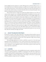
unit time to fetch the first instruction at the destination address. The fetch-execute cycle of the SPARC
processor is illustrated in Figure 3.1 (this is simplified slightly, as we will see shortly).

3.2.1

Annulled Branches

</div>
<span class='text_page_counter'>(28)</span><div class='page_container' data-page=28>

Figure 3.1: Simplified SPARC Fetch-Execute Cycle

within a loop is moved to the delay slot but should not be executed on the last iteration of the loop. If
a conditional branch is annulled then the instruction in the delay slot is executed only if the branch is
taken. If the branch is not taken (execution falls through to the code following the branch instruction)
then the execution of the instruction in the delay slot is annulled (ignored). Note, however, that a clock
cycle is “wasted”, as the pipeline does no useful work for a cycle when an instruction is annulled in this
way (in effect, it is as if the delay slot instruction has become anop). In order to specify that a branch is
to be annulled we simply follow the mnemonic for the branch with ana(for example, ble,a loop). We
will consider an example of the use of this feature shortly.

In addition, unconditional branches can also be annulled. In this case the effect of annulling the instruction
has the opposite effect: the instruction in the delay slot is never executed. This effectively provides a
single instruction branch operation in which the delay slot has no effect. The main use of this is to allow
one to replace an instruction with a branch to an emulation routine without changing the semantics of the
program. The full fetch-execute cycle of the SPARC processor incorporating the possibility of annulled
branches is shown in Figure 3.2.

3.3

An Example — Looping

We will extend the example program from the previous chapter so that it calculates the Fahrenheit
equivalents of temperatures from 10<i>◦</i>_{C to 20}<i>◦</i>_{C. In C or Java we could express the algorithm as follows:}

for (c = 10; c < 21; c++)
f = 9/5 * c + 32;
Or, more explicitly, as:

</div>
<span class='text_page_counter'>(29)</span><div class='page_container' data-page=29>

Figure 3.2: SPARC Fetch-Execute Cycle

{ f = 9/5 * c + 32;
c++;

}

while (c < 21);

If we model our assembly language program on the latter algorithm we will need to use a conditional
branch instruction at the end of the loop. Otherwise the program is much as it was before.

/* This program converts temperatures between 10 and 20 in
Celcius to Fahrenheit.

George Wells - 30 May 2003
*/

offs = 32

/* Variables c and f are stored in %l0 and %l1 */
.global main

main:

mov 10, %l0 ! Initialize c = 10
loop:

mov 9, %o0 ! 9 into %o0 for multiplication
call .mul ! Result in %o0

mov %l0, %o1 ! c into %o1 for multiplication
call .div ! Result in %o0

</div>
<span class='text_page_counter'>(30)</span><div class='page_container' data-page=30>

add %o0, offs, %l1 ! f = result + offs
add %l0, 1, %l0 ! c++

cmp %l0, 21 ! c < 21 ?

bl loop

nop ! Delay slot

mov 1, %g1 ! Trap dispatch

ta 0 ! Trap to system

Thecmpinstruction used in this program is another example of a synthetic instruction. The assembler
translates this intosubcc %l0, 11, %g0(note the use of g0as the destination register here). Similarly,
we could have used the syntheticincinstruction instead of the explicit additionadd %l0, 1, %l0. In the
gdbdisassembly of the program below we will see thatgdbhas interpreted the addition as the synthetic
instruction.

To check the execution of this program we can use the following set of steps ingdb:
$ gdb a.out

...

(gdb) b *main

Breakpoint 1 at 0x10a80
(gdb) display $l0
(gdb) display $l1
(gdb) r

Starting program: /home/csgw/Cs4/Arch/Misc/Ch2/a.out

(no debugging symbols found)...(no debugging symbols found)...
Breakpoint 1, 0x10a80 in main ()

2: $l1 = 268576604
1: $l0 = 268675072

(gdb) disass main main+100

Dump of assembler code from 0x10a80 to 0x10ab4:
0x10a80 <main>: mov 0xa, %l0

0x10a84 <loop>: mov 9, %o0

0x10a88 <loop+4>: call 0x20c48 <.mul>
0x10a8c <loop+8>: mov %l0, %o1

0x10a90 <loop+12>: call 0x20c54 <.div>
0x10a94 <loop+16>: mov 5, %o1

0x10a98 <loop+20>: add %o0, 0x20, %l1
0x10a9c <loop+24>: inc %l0

0x10aa0 <loop+28>: cmp %l0, 0x15
0x10aa4 <loop+32>: bl 0x10a84 <loop>
0x10aa8 <loop+36>: nop

0x10aac <loop+40>: mov 1, %g1 ! 0x1
0x10ab0 <loop+44>: ta 0

End of assembler dump.
(gdb) b *main+28

Breakpoint 2 at 0x10a9c
(gdb) c

Continuing.

</div>
<span class='text_page_counter'>(31)</span><div class='page_container' data-page=31>

2: $l1 = 50
1: $l0 = 10
(gdb) c
Continuing.

Breakpoint 2, 0x10a9c in loop ()
2: $l1 = 51

1: $l0 = 11
(gdb) c
Continuing.

Breakpoint 2, 0x10a9c in loop ()
2: $l1 = 53

1: $l0 = 12
(gdb)
Continuing.

Breakpoint 2, 0x10a9c in loop ()
2: $l1 = 55

1: $l0 = 13
(gdb)
Continuing.

Breakpoint 2, 0x10a9c in loop ()
2: $l1 = 57

1: $l0 = 14
(gdb)

Exercise 3.1 Satisfy yourself that this program is working correctly.

'

&

$

%

Useful Hint

If a file called.gdbinitis found in a user’s home directory thengdbwill
automati-cally execute any commands found in this file when it starts up. For example, it is
useful to have something like the following:

break *main
display/i $pc
r

</div>
<span class='text_page_counter'>(32)</span><div class='page_container' data-page=32>

loop:

mov 9, %o0 ! 9 into %o0 for multiplication
call .mul ! Result in %o0

mov %l0, %o1 ! c into %o1 for multiplication
call .div ! Result in %o0

mov 5, %o1 ! 5 into %o1 for division
add %l0, 1, %l0 ! c++

cmp %l0, 21 ! c < 21 ?

bl loop

add %o0, offs, %l1 ! f = result + offs

This sort of rearrangement of the program is not particularly easy for us as human programmers. It
also complicates the debugging and maintenance of the program as it distorts the natural order of the

algorithm. Fortunately these optimisations are relatively easy for a good compiler to perform, and can
produce very efficient programs.

3.4

Further Examples — Annulled Branches

3.4.1

A While Loop

Consider the following segment of a C program.
while (x < 10)

x = x + y;

Converting this to assembly language, we might come up with something like the following:
! Assumes x is in %l0 and y is in %l1

b test ! Test if loop should execute

nop ! Delay slot

loop: add %l0, %l1, %l0 ! x = x + y
test: cmp %l0, 10 ! x < 10

bl loop ! If so branch back to loop start

nop ! Delay slot

Here the first delay slot is only executed once (when the loop is entered) and so is of little consequence.
The second delay slot is more important since it will be executed on every iteration of the loop. The only
instruction that is a candidate for this delay slot is the add instruction. At first, moving this into the
delay slot may appear incorrect, as it appears to move the addition to after the comparison, but in fact

(due to the way in which the loop is structured and the delay slot is used) it will work much as expected.
The problem arises whenxbecomes greater than or equal to 10 (or if xis greater than or equal to 10 at
the start of the execution of this program segment). In this case the addition will be executed one time
too many. The delay slot can be annulled to overcome this, as shown below.

</div>
<span class='text_page_counter'>(33)</span><div class='page_container' data-page=33>

b test ! Test if loop should execute

nop ! Delay slot

loop:

test: cmp %l0, 10 ! x < 10

ble,a loop ! If so branch back to loop start
add %l0, %l1, %l0 ! x = x + y; delay slot

Note how tight this code is. Again, this sort of optimisation is not particularly easy for a human
programmer to construct or to follow, but good optimising compilers can easily perform these sorts of
rearrangements.

3.4.2

An If-Then-Else Statement

The classic if-then-else statement also gives much scope for the use of annulled branches and delay slots.
Consider the following segment of a C program:

if (a + b >= c)
{ a += b;

c++;
}

else

{ a -= b;
c--;
}

Converting this directly into assembly language we might come up with something like the following:
! Assume a => %l0, b => %l1, c => %l2

! and %o0 is used as a temporary store

add %l0, %l1, %o0 ! tmp = a + b

cmp %o0, %l2 ! Compare tmp with c
bl else ! if tmp < c then goto else clause

nop ! Delay slot

! Then clause

add %l0, %l1, %l0 ! a += b
add %l2, 1, %l2 ! c++

b next ! Jump over else clause

nop ! Delay slot

else: sub %l0, %l1, %l0 ! a -= b
sub %l2, 1, %l2 !
c--next:

</div>
<span class='text_page_counter'>(34)</span><div class='page_container' data-page=34>

add %l0, %l1, %o0 ! tmp = a + b

cmp %o0, %l2 ! Compare tmp with c

bl,a else ! if tmp < c then goto else clause
sub %l0, %l1, %l0 ! a -= b; Delay slot; Else code
! Then clause

add %l0, %l1, %l0 ! a += b

b next ! Jump over else clause
add %l2, 1, %l2 ! c++; Delay slot
else: sub %l2, 1, %l2 !

c--next:

Exercise 3.2 Write a program to find the maximum value of the function
<i>x</i>3<i>₋</i>_14x2_{+ 56x}<i>₋</i>₆₄

in the range<i>−2≤x≤</i>8, in steps of one. Usegdbto find the result.

Exercise 3.3 Write a program to calculate the square root<i>y</i>of a number<i>x</i>using the
Newton-Raphson method. This method uses the following algorithm:

y = x / 2
repeat

{ old = y

dx = x - y * y
y = y + dx / 2y
} until y == old

Test your program usinggdbto ensure that it works correctly.

Skills

<i>•</i> You should understand the basic concepts of pipelining and pipeline stalls

</div>
<span class='text_page_counter'>(35)</span><div class='page_container' data-page=35>

Chapter 4

Logical and Arithmetic Operations

Objectives

<i>•</i> To study the basic arithmetic and logical operations provided by the SPARC architecture
<i>•</i> To consider the provision of multiplication and division operations, including the use of

stan-dard subroutines

As is the case with most modern processors, the SPARC architecture has a large set of logical and
arithmetic operators. In this chapter we will be studying these in more depth.

4.1

Logical Operations

The logical operations supported by the SPARC processor fall into two categories: <i>bitwise logical </i>
<i>opera-tions</i>and<i>shift operations</i>. We will consider each of these separately.

4.1.1

Bitwise Logical Operations

Table 4.1 details the logical operations provided by the SPARC architecture. There are instructions for
the usual bitwise logical operations of and, or and exclusive or. In addition it has some rather less
usual operations (the last three in Table 4.1). These operations all have the three-address format common
to most of the SPARC instructions.

The other useful boolean operations of nandandnormust be constructed from anandororoperation
followed by a notoperation. The notoperation is not directly supported, but is synthesised from the
xnor operation, using the zero register: xnor %rs, %g0, %rd. Bothnot %rs, %rd and not %rs<i>/</i>d are

recognised by the assembler for this purpose.

In addition to the basic forms of these instructions, there are variations on them that set the condition
flags. As we have seen before, these use the same mnemonic but withccas a suffix (for example,andcc).
If we simply want to set the flags according to a value stored in a register we can use the zero register and
anoroperation to do this. The instructionorcc %rs, %g0, %g0 will effectively set the flags according

</div>
<span class='text_page_counter'>(36)</span><div class='page_container' data-page=36>

Function Description
and

or
xor

xnor <i>a</i>xnor<i>b</i> = not(axor<i>b)</i>

andn <i>a</i>andn<i>b</i> = <i>a</i>and not(b)

orn <i>a</i>orn<i>b</i> = <i>a</i>or not(b)
Table 4.1: Logical Instructions

instruction will not change any of the values in the registers, only the condition codes). As this is a useful
instruction it is also available as a synthesised instruction called tst. We could use this instruction as
shown in the following program segment:

/* Assembler code for
if (a > 0)

b++;

Assumes a is in %l0 and b in %l1 */

tst %l0 ! Set flags according to a
ble next ! Skip if a <= 0

nop

inc %l1 ! b++

next:...

4.1.2

Shift Operations

The SPARC architecture has three different shift operations. These fall into two classes: arithmetic shift
operations and logical shift operations. The difference between the two classes concerns the handling of
the sign bit. When performing an arithmetic shift to the right (sra) the sign bit is duplicated on each
shift. For a logical right shift (srl) zeroes are fed in to the most significant bit. There is no difference
when considering left shifts, as zeroes can be fed into the least significant bit position in both cases,
and only a single opcode (sll) is provided. As we know from binary number theory, shifting to the left
corresponds to multiplication by powers of two and shifting to the right corresponds to division by powers
of two.

Since the largest shift that makes any sense is 31 bit positions the number of bits to be shifted is taken
from the low five bits of either an immediate value or the second source register. The use of the shift
operations is illustrated in the following code segment:

! Assumes a => %l0, b => %l1, c => %l2

sll %l0, %l1, %l2 ! c = a << b

sra %l0, 2, %l1 ! b = a >> 2, i.e. b = a / 4

</div>
<span class='text_page_counter'>(37)</span><div class='page_container' data-page=37>

Operation Description

add Add

addcc Add and set flags

addx Add with carry

addxcc Add with carry and set flags

sub Subtract

subcc Subtract and set flags

subx Subtract with carry

subxcc Subtract with carry and set flags
Table 4.2: Arithmetic Instructions

4.2

Arithmetic Operations

The SPARC architecture has a small set of arithmetic operations. Essentially there are only addition and
subtraction operations defined. We have seen both of these in use already and have mentioned that there
are variations that set the integer condition codes. One variation that we have not yet seen is to include
the carry flag in the addition or subtraction. The full set of normal arithmetic operations supported by
the SPARC is shown in Table 4.2. These have the usual three-address format.

4.2.1

Multiplication

The first generation of SPARC processors did not have multiplication and division instructions in the
instruction set (we have seen already how we can perform these operations by calling on the standard
subroutines.muland.div). However, multiplication was supported indirectly by means of the multiply
step instruction (mulscc). This instruction allows us to perform long multiplication simply by following
a number of steps.

Long Multiplication

Before looking at the use of the mulsccinstruction, we need to consider how binary long multiplication
is performed “by hand”. Let us consider the example of multiplying 5 (101) by 3 (11), using four bits
(the result will then need eight bits). We start off with a partial product of 0. The algorithm works as
follows.

dofour times

if the least significant bit of the multiplier is 1then

add the multiplicand into the high part of the partial product
endif

shift the multiplier and the partial product one bit to the right
enddo

This last step can conveniently be taken care of by storing the multiplier in the low part of the partial
product and shifting them all together. As this is done four times (in our example — in general it is done
as many times as there are bits in a word) the multiplier will be completely shifted out by the time we
are finished. Let’s look at our example.

Multiplicand: 0011
Multiplier: 0101

</div>
<span class='text_page_counter'>(38)</span><div class='page_container' data-page=38>

Step 1: low bit of partial product is one so add multiplicand into high part
partial product becomes 0011 0101

shift right; partial product becomes 0001 1010
Step 2: low bit of partial product is not one

partial product remains 0001 1010

shift right; partial product becomes 0000 1101

Step 3: low bit of partial product is one so add multiplicand into high part
partial product becomes 0011 1101

shift right; partial product becomes 0001 1110
Step 4: low bit of partial product is not one

partial product remains 0001 1110

shift right; partial product becomes 0000 1111

At this point we are finished. The result (0000 1111) is the binary representation of 15, which is extremely
comforting! Essentially we have traced out the following multiplication (written in a more conventional
style):

0011×
0101
0011
1100
1111

The only other point we need to worry about concerns the case when the multiplier is negative. We can
proceed almost exactly as above. The shift operations must be signed, arithmetic shifts (as opposed to
logical shifts). Also, in order to correct the final result, we need to subtract the multiplicand from the
high part of the last partial product. With these enhancements the complete algorithm is as follows.

dofour times

if the least significant bit of the multiplier is 1then

add the multiplicand into the high part of the partial product
endif

shift the multiplier and the partial product one bit to the right
enddo

if the multiplier is negativethen

subtract the multiplier from the high part of the partial product
endif

Exercise 4.2 Try multiplying<i>−3 by 5 and−3 by−5, using a four bit word, and confirm the</i>
action of this algorithm. From what does the need to correct the final result in the case of a
negative multiplier arise?

The SPARC Multiplication Step Instruction

With the knowledge of how binary multiplication can be performed behind us we can turn to the SPARC
mulsccinstruction. This performs the repetitive step in the above algorithm, using the specialYregister
as the low part of the partial product. The format of the instruction is: mulscc %rs1, %rs2, %rd, where

</div>
<span class='text_page_counter'>(39)</span><div class='page_container' data-page=39>

and the destination register (%rd) should be the same register, and should be the high word of the partial

product. The sequence of steps required to perform a multiplication on a SPARC processor is then as
follows:

1. The multiplier is loaded into the%Yregister (the low word of the partial product) and the register
to be used for the high word of the partial product is cleared to zero.

2. The multiplier is tested to set theN(negative) andV(overflow) bits.

3. Thirty-twomulsccoperations are performed. Each of these steps shiftsN ^ Vinto the most
signif-icant bit of %rs1, shifting all the other bits to the right and saving the least significant bitb. The

least significant bit of the Y register is tested, and if it is one the second source register (or sign
extended constant) is added to the destination register. Lastly, the saved bit bis shifted into the
left end of theYregister and all the other bits are shifted one place to the right.

4. One lastmulsccis performed with the multiplicand set to zero to perform the last right shift giving
the final result (high word in the destination register and low word in theYregister).

5. If the multiplier was negative it must be subtracted from the high word of the result.

So, to multiply 3 (in%l0) by 5 (in %l1), using %o1for the high part of the partial product we could use
the following segment of assembler code.

mov 3, %l0
mov 5, %l1
mov %l1, %y

andcc %g0, %g0, %o1 ! Clear high word of partial
! product and clear flags

mulscc %01, %l0, %o1 ! 32 mulscc instructions no. 1
mulscc %01, %l0, %o1 ! no. 2

...

mulscc %01, %l0, %o1 ! no. 31
mulscc %01, %l0, %o1 ! no. 32
mulscc %o1, %g0, %o1 ! Final shift

mov %y, %o0 ! Get low order part from Y reg.
Note that themulsccinstruction modifies the flags, as implied by the ccsuffix.

Exercise 4.3 Code this up into an assembly language program and trace through to see how
it works. Try a few more values for multiplier and multiplicand. Extend the program to allow
for signed multipliers and check that this works as expected too.

As we have seen already there is a standard subroutine provided to perform multiplication (.mul). This

performs signed multiplication. If the values that are being multiplied are unsigned the .umul routine
should be used instead. Both of these take the multiplicand in %o0and the multiplier in%o1. The low
word of the result is returned in%o0and the high order part in%o1.

4.2.2

Division

</div>
<span class='text_page_counter'>(40)</span><div class='page_container' data-page=40>

for various division operations. These fall into two classes: signed operations and unsigned operations.
Considering the signed operations first, .div returns the quotient while .rem returns the remainder.
Similarly,.udivand.uremare provided for unsigned division. All of these take the dividend in the %o0
register and the divisor in the%o1register. The result is returned in%o0in all cases.

Exercise 4.4 Look up a binary division algorithm (such as that in Wakerley[24, p. 101 ff.])
and implement it in SPARC assembly language.

Skills

<i>•</i> You should know the basic arithmetic and logical operations

<i>•</i> You should understand the reason for the provision of themulsccoperation and have a basic
understanding of its use

</div>
<span class='text_page_counter'>(41)</span><div class='page_container' data-page=41>

Chapter 5

Data Types and Addressing

Objectives

<i>•</i> To introduce the basic SPARC data types

<i>•</i> To study the organisation of data in registers and in memory

<i>•</i> To consider the addressing modes provided by the SPARC architecture
<i>•</i> To introduce the concept of<i>register windowing</i>

<i>•</i> To study the use of global data

In this chapter we will start off by taking a look at the various data types that are supported by the SPARC
architecture and also at the addressing modes available. The SPARC processor has fewer addressing
modes than CISC processors like the Intel 80x86 family. This background leads us naturally onto the
subject of where, and how, to store variables in our programs, and introduces the concepts of <i>register</i>
<i>windows</i>.

5.1

SPARC Data Types

The SPARC processors support eleven data types. These are byte, unsigned byte, halfword, unsigned
halfword, word, unsigned word, doubleword, tagged data and single-, double- and extended-precision
floating point. The characteristics of these types are shown in Table 5.1.

For simplicity, we will refer to data types less than 32 bits wide as<i>short</i> types (i.e. the byte types and
halfword types) and will refer to data types greater than 32 bits wide as<i>long</i> types.

5.1.1

Data Organisation in Registers

</div>
<span class='text_page_counter'>(42)</span><div class='page_container' data-page=42>

Type Size Corresponding Range
(bits) C Data Type

Unsigned Byte 8 unsigned char 0. . . 256

Byte 8 char -128. . . 127

Unsigned Halfword 16 unsigned short 0. . . 65 535

Halfword 16 short -32 768. . . 32 767

Unsigned Word 32 unsigned int/long 0. . . 4 294 967 295

Word 32 int/long -2 147 483 648. . .

2 147 483 647

Doubleword 64 N/A -9 223 372 036 854 775 808. . .

9 223 372 036 854 775 807

Tagged Data 30+2 N/A 0. . . 1 073 741 823

Single Precision 32 float s = 1, e = 8, f = 23

Floating Point

Double Precision 64 double s = 1, e = 11, f = 52

Floating Point

Extended Precision 128 N/A s = 1, e = 15, j = 1, f = 63

Floating Point

For floating point values:

s is the number of sign bits,

e is the number of bits for the exponent,

f is the number of bits for the fractional part, and

j is the number of bits for the integer part (single and double precision floating point values are
stored in a normalised format that makes this unnecessary).

Table 5.1: SPARC Data Types

data types (i.e. the sign bit is duplicated through the unused bits of the register). The unsigned short
data values have zeroes stored for the unused bits. When storing a value in memory, the unused upper
bits of a short data type are discarded.

The long data types (doubleword and double precision floating point values) require two registers for
storage. The most significant word is stored in the lower numbered register and the least significant
word in the higher numbered register. In these cases the destination register for an operation must be an
even numbered register. If it is not then the processor forces an even numbered register by subtracting
one from the specified register number. For example, attempting to load a doubleword value into either
registeri6ori7will result in the value being stored in registersi6andi7. Extended precision
floating-point values require four registers. Again, an even numbered register must be used as the destination for
an extended precision value. Note that storing a long data value into registerg0will result in the most
significant word being lost — the least significant word will be stored ing1.

Floating Point Values

Floating point values may be stored either in the registers of the integer unit or in the registers of the
floating-point coprocessor. There are thirty-two of these called f0throughf31, each 32 bits wide. We
will not be considering the floating-point coprocessor in any detail in this course.

</div>
<span class='text_page_counter'>(43)</span><div class='page_container' data-page=43>

contain the exponent and the remainder of the word contains the fraction. For double precision
floating-point types the most significant word (stored in the lower numbered register) contains the sign bit (bit
31), the eleven bit exponent (bits 20 through 30) and the high-order 20 bits of the fraction. The least
significant word contains the low-order bits of the fraction.

Tagged Data Types

The tagged data types have been touched on briefly already. They are stored using the most significant
30 bits for the value and the least significant 2 bits for a <i>tag</i>. The tag bits are used to indicate the
type of the data from an application program’s perspective. Tagged data values are of great use when
implementing functional and logical languages such as Haskell, LISP, Smalltalk, Prolog and RUFL1_{. The}

instructions that deal with tagged data (taddccandtsubcc) will set the overflow flag if the tag of either
operand is nonzero (or if normal overflow occurs). For this reason tagged operations are usually followed
by a conditional branch to a routine that will check the format of the operands. To make this even easier
there are special forms of the tagged operations (taddcctv andtsubcctv) that automatically perform
a trap (similar to a software interrupt) if the overflow bit is set during the execution of the operation.
Other than this, tagged data values are treated as normal unsigned values when manipulated by the
processor.

5.1.2

Data Organisation in Memory

The Big-Endian Convention

The SPARC architecture uses the<i>big-endian</i>convention, rather than the<i>little-endian</i>convention used by
the Intel 80x86 family of processors. The SPARC addressing scheme thus stores the higher-order bytes
of multi-byte values at the lower memory addresses. For example, a word value (i.e. four bytes) stored in
memory will have the most significant byte stored at address<i>N</i> and the least significant byte stored at
address<i>N</i>+ 3. The address of any data value is thus the address of its most significant byte. In general,
this distinction is not important, unless one tries to retrieve multi-byte values in smaller size units (e.g.

retrieving a four-byte word value as four individual bytes).

Address Alignment

In addition, all data values<i>must</i> be aligned on address boundaries that are an exact multiple of the data
size (this provides greater efficiency for memory accesses). The aligment restrictions mean that halfword
values must be located at even addresses (i.e. divisible by two). Similarly, word values must be stored
on word boundaries (the address exactly divisible by four, or the low two bits of the address set to zero),
and doubleword values must be stored on doubleword boundaries (the address exactly divisible by eight,
or the low three bits of the address set to zero).

Note that the same alignment restrictions apply to instructions being fetched from memory. The
impli-cation of this is that all instructions <i>must</i> appear at addresses that are exact multiples of four (i.e. the
least signficant two bits of instruction addresses will always be zero).

Any attempt to access a data value or instruction using an address that is not properly aligned will result
in a hardware trap being generated. By default, this will be caught by the operating system and the
offending program will be terminated with an error message, as shown in the following example.

$ myprog

</div>
<span class='text_page_counter'>(44)</span><div class='page_container' data-page=44>

5.2

Addressing Modes

The SPARC architecture uses 32-bit addresses for memory accesses. This address size gives an address
space of 4 294 967 295 bytes (i.e. 4GB, enough for most applications!). There are only four addressing
modes supported by the SPARC processors: two-register, register plus immediate, 30-bit program counter
relative and 22-bit program counter relative. The small number of addressing modes is mainly because of
the simplified load/store architecture of the SPARC. Memory addressing is performed only for load and
store instructions and for control transfers. We will consider each of the four addressing modes in turn.

5.2.1

Data Addressing

Two Register Addressing

This addressing mode uses the values contained in two registers in order to generate an address. The
two values are added together to create the address, which is then used to load or store a value from/to
memory. These addresses are a full 32 bits wide.

Register Plus Immediate Addressing

This addressing mode makes use of a 32-bit value from a register together with a sign-extended 13-bit
immediate value. These two components are added together to give the effective address. As a special
case of this addressing mode, the zero register g0 can be used, giving a 13-bit immediate addressing
mode that can be used to access the upper and lower 4kB of memory (effectively this is like an absolute
addressing mode for these regions of memory). This is the simplest addressing mode since no registers
need to be specially set up beforehand.

5.2.2

Control Transfer Addressing

Thirty Bit Program Counter Relative Addressing

This addressing mode is used only by the call instruction. A 30-bit displacement (taken from the
instruction) is padded to 32 bits by appending two zero bits and the result is added to the program
counter (in fact, due to the way in which the fetch-execute cycle works, the value that is used isPC+ 4).
This results in no loss of functionality, since the SPARC instructions are all 32 bits wide, and therefore
must be fetched from word aligned addresses in which the lower two bits will always be zero. This
addressing mode thus allows transfer of control to any instruction in the entire address space of the
processor. The calculated address (known as the <i>effective address</i>) becomes the new value of the nPC
register.

Twenty-two Bit Program Counter Relative Addressing

</div>
<span class='text_page_counter'>(45)</span><div class='page_container' data-page=45>

5.3

Stack Frames, Register Windows and Local Variable

Stor-age

When a program is loaded into memory by the operating system the code is located at low addresses
and a stack is located at the top end of the memory space. The address of the last occupied stack
memory element is stored in the <i>stack pointer</i>, register o6or sp (its preferred name). If we wanted to
set aside some stack space for local variables we could simply decrement the stack pointer by the number
of bytes that we require. For example, to reserve 64 bytes of memory we could execute the instruction
sub %sp, 64, %sp. One point to note is that the stack should always be kept doubleword aligned, and
for this reason the lowest three bits of the stack pointer should always be zero (i.e. the stack pointer
should always be exactly divisible by eight). So, if we required 94 bytes of memory for local storage, then
we would need to decrement the stack pointer by 96 in order to keep the stack aligned. There is a useful
shortcut that can be used to ensure that this is always true. The trick is to add a negative number to
the stack pointer rather than subtracting a positive value, and then to mask off the lowest three bits of
this value. So, instead of sub %sp, 94, %sp, we would writeadd %sp, -94 & 0xfffffff8, %sp. The
hexadecimal constant 0xfffffff8 is the two’s complement representation of -8 and so we can write this a
little more concisely, if a little less clearly, asadd %sp, -94 & -8, %sp.

Exercise 5.1 Try a few examples and convince yourself that this shortcut works. Why does
it work?

The stack pointer frequently changes during the execution of a program and is less than satisfactory as
the basis for addressing variables. To solve this problem we use a<i>frame pointer</i>, register i6, also called
fp. The frame pointer is used to hold a copy of the stack pointer before its value is changed to provide
more storage. To see how the frame pointer is set up we need to turn to the subject of<i>register windows</i>,
an important architectural feature of the SPARC processors.

5.3.1

Register Windows

Earlier when we introduced the subject of the registers available to the programmer we said that there
were thirty-two registers available at any time, eight global registers and twenty-four window registers.
These twenty-four window registers are taken from a large pool of registers (typically 128, which is
the number we will assume in the following discussion). The window registers are arranged into eight
overlapping groups called<i>windows</i>, as illustrated in Figure 5.1. The eight “out” registers of one window
are the “in” registers of the next window and so on. Only the local registers are truly private to any one
window. The current working window is indicated by a 5-bit field in the program status register (visible
only in supervisor mode) called the<i>current window pointer</i>(CWP). This allows for a maximum of
thirty-two windows (a total of 512 potential registers) on SPARC processors. The window registers are treated
as a circular stack with the highest numbered window adjoining the lowest. Decrementing the CWP
moves to the next window in the set, and incrementing the CWP moves back to the previous window.
The CWP may be manipulated by means of thesave and restore instructions, which decrement and
increment the CWP respectively. These instructions bring us back to the subject of the frame pointer,
so let’s take a look at them in more detail.

Manipulating the Register Window

</div>
<span class='text_page_counter'>(46)</span><div class='page_container' data-page=46>

Figure 5.1: Register Window Layout
[19, p. 2-3]

frame very simply, as shown below. In this example, we assume that we want to set aside space for five
word-long (i.e. four byte) variables.

save %sp, -64 - (5 * 4) & -8, %sp

The need for the extra 64 bytes of storage we will consider shortly. This instruction is most easily
understood by considering the special registers spandfpas normal “in” and “out” registers. The first
reference tospis a reference to registero6of the “old” window. The destination registerspis then the
registero6of the “new” window, while the “old”spis still visible as the registeri6, which, conveniently,
is the frame pointer register. So, the stack looks as shown in Figure 5.2 (the five local variables have

been labelledv1throughv5for clarity). In order to access the variables stored on the stack we can use
negative offsets from the frame pointer. In passing, note that the expression -64 - (5 * 4) & -8 is
evaluated by the assembler when it is assembling the text of the program.

</div>
<span class='text_page_counter'>(47)</span><div class='page_container' data-page=47>

Figure 5.2: Example of a Minimal Stack Frame

Register Window Overflow and Underflow

Returning to the subject of the extra 64 bytes set aside in the above example, these are used to store
the contents of the registers when there is a<i>window overflow</i>. This occurs when a program attempts to
make use of more than the available number of windows. The way in which this is handled is that a
window can be marked as invalid (by setting a bit in the Window Invalid Mask register or WIM register,
available only in supervisor mode). If an attempt is made to perform asaveto an invalid window a trap
is generated automatically. At the same time as the trap the CWP is decremented anyway, allowing the
trap handler (usually part of the operating system) to make use of the invalid window. The trap handler
is then responsible for freeing up a window by saving the local registers and out registers for the next
window, which is then marked as invalid, the current window is remarked as valid and control is returned
to the program. In this way an executing program effectively sees an infinite number of windows. The
saved registers are stored in the extra 64 bytes allocated on the stack frame. If your programs do not set
aside this space and a window overflow trap is generated then chaos is guaranteed to result!

Similarly, a window underflow trap is generated if arestoreinstruction attempts to increment the CWP
to point to a window marked as invalid. In this case, the trap handler would restore the contents of a
window that had previously been saved into the stack frame.

This mechanism is particularly well suited to parameter passing between subroutines, a subject to which
we will return in the next chapter.

5.3.2

Variables

</div>
<span class='text_page_counter'>(48)</span><div class='page_container' data-page=48>

Name Data Type Description

ldsb Signed Byte Load 8 bit value, sign extended

ldub Unsigned Byte Load 8 bit value

ldsh Signed Halfword Load 16 bit value, sign extended

lduh Unsigned Halfword Load 16 bit value

ld Word Load 32 bit value

ldd Doubleword Load 64 bit value into 2 registers

stb Byte Store low 8 bits of register

sth Halfword Store low 16 bits of register

st Word Store 32 bit register

std Doubleword Store 2 registers as 64 bits
Table 5.2: Load and Store Instructions

The load instructions have two operands2_{. The first of these is the address specification, enclosed in}

square brackets []to indicate that it is an address not a data value. The second operand is the name
of the register in which the loaded value is to be stored. The store instructions also take two operands,
which are the same as those for the load instructions, but with their order reversed.

As an example, the following program segment moves a data value from one memory location to another.

save %sp, -64 -(2 * 4) & -8, %sp ! Space for 2 vars, a and b

...

ld [%fp - 4], %l0 ! l0 <- a
st %l0, [%fp - 8] ! b <- l0

Here, both theldand thestinstructions are using the register-plus-immediate addressing mode discussed
on page 37.

When accessing variables in this way we need to keep a close track of the locations we are allocating to
specific variables. We can simplify this by making use of the facilities of the macro processorm4. If we
define the macroslocal varsandvaras shown below, we can automate a lot of the work.

define(local_vars, ‘define(last_sym, 0)’)

define(var, ‘$1 = last_sym $2 & $2 define(‘last_sym’, $1)’)

The local vars macro simply initialises a macro token called last sym to have the value zero. The
macrovarcan best be understood perhaps by considering an example. If we writevar(a, 4)to allocate
space for a word (four byte) variable calleda, this would be expanded out first to read:

a = last_sym - 4 & -4 define(‘last_sym’, a)

This contains several macro names itself and so will be expanded again to give the final result:
a = 0 - 4 & -4

and the tokenlast symwill have the new valuea. Note that none of this has yet allocated any memory
to be used for the variable. When we come to declare the next variable (say a halfword value called b)
we would give a definition likevar(b, 2). This would then be expanded out to:

2_{Actually there are three operands, as the load/store instructions are still triadic (three-address) instructions, but the}

</div>
<span class='text_page_counter'>(49)</span><div class='page_container' data-page=49>

b = a - 2 & -2

withlast symnow having a value ofb. Notice how ensuring the correct alignment is quite straightforward
since the size of the data value also gives the alignment value. The expressions like 0 - 4 & -4 and
a - 2 & -2are left for the assembler to evaluate.

Two more useful macros, shown below, allow us to simplify the start and end of our assembly language
programs. Note how we can use the value of last symin working out how much space is required for
variables in the stack frame. It is at this point (using thebeginmacro) that memory is allocated on the
stack for the variables declared above.

define(begin, ‘.global main

main: save %sp, -64 + last_sym & -8, %sp’)
define(end, ‘ mov 1, %g1

t 0’)

These macros allow us to write far more readable programs, as in the following variation of the previous
example.

local_vars
var(x, 4)
var(y, 4)
begin

ld [%fp + x], %l0 ! l0 <- x

st %l0, [%fp + y] ! y <- l0
end

After being processed bym4this example will appear as follows:
x = 0 - 4 & -4

y = x - 4 & -4
.global main

main: save %sp, -92 + y & -8, %sp

ld [%fp + x], %l0 ! l0 <- x
st %l0, [%fp + y] ! y <- l0
mov 1, %g1

t 0

To make matters even simpler still we can put these macros into a file and include this file in any programs
that make use of the macros. This can be done by using them4 includemacro as shown in the following
complete (but useless) program.

include(macro_defs.m)
local_vars

</div>
<span class='text_page_counter'>(50)</span><div class='page_container' data-page=50>

ld [%fp + x], %l0 ! l0 <- x
st %l0, [%fp + y] ! y <- l0
end

The filemacro defs.m, containing these and other useful macros, can be found on the Sun systems in
the directory /home/cs4/Arch.

5.4

Global Variables

In addition to local variables, which we can handle using the stack as shown above, the assembler allows
us to define global variables using pseudo-ops.

5.4.1

Data Declaration

There are several data definition pseudo-ops available to us for use with the different data types. The
simplest of these is.wordwhich allows us to allocate space for a 32 bit variable, and initialise its value.
Similarly, the.byteand.halfdirectives allow us to allocate space for bytes and halfwords respectively.
Since the data values must be correctly aligned in memory, another important pseudo-op in this context is
.alignwhich enforces the alignment. If we want to set aside a given amount of space without initialising
it we can use the.skipdirective to allocate space for a specified number of bytes.

These points are all illustrated by the following program extract.
.data ! Start data segment

x: .word 12 ! int x = 12;

y: .byte ’a’ ! char y = ’a’;

.align 2 ! Get alignment correct for halfword
z: .half 0xffff ! short z = 0xffff;

.align 4 ! Get alignment correct for words
list: .skip 4 * 100 ! int list[100];

.text ! Start of program segment
. . .

Note that the data and program segments referred to here are <i>not</i> related to the Intel 80x86 concept
of a segment. The UNIX operating system splits all programs into sections, called segments. The first
of these is the <i>text segment</i> into which all program code is placed. This is usually made read-only so
that it can be shared among all processes executing the same code. The<i>data segment</i>that we have seen
used above is where data is placed. The data segment is loaded by the operating system as a read/write
segment, and is generally not shared between processes.

If we are going to make use of separate assembly and linking different modules together then we need to
use the.globalpseudo-op to “export” any variable names we want visible to other parts of the system.
This is just as it is in C, of course. Similarly, if we wantgdb to recognise the identifier names then we
must also declare them as global. This is shown in the following program extract.

.data ! Start data segment
.global x ! Export x

x: .word 12 ! int x = 12;

y: .byte ’a’ ! char y = ’a’;

</div>
<span class='text_page_counter'>(51)</span><div class='page_container' data-page=51>

.align 4 ! Get alignment correct for words
.global list ! Export list

list: .skip 4 * 100 ! int list[100];
.text

In this example, the identifiersxandlistwill be visible to other object files that are linked with this one
and will also be visible to the debugger. The other variables,yand z, will be visible within the module
within which they appear, but will not be accessible from other modules, nor will their names be known
bygdb.

Lastly, we turn to the subject of character strings. These can be defined by listing the ASCII codes as
follows:

str: .byte 150, 145, 154, 154, 157

Alternatively, and more conveniently, we can use the characters themselves by enclosing them in quotes
(either single or double quotes).

str: .byte "h", "e", "l", "l", "o"

However, this is still rather tedious, and so the assembler provides two other data definition pseudo-ops
for use with character strings. These are .asciiand .asciz. They both take a character string as an
argument and set aside enough space for the string initialised to the ASCII values of the characters in
the string. The difference between the two pseudo-ops is that the.ascizpseudo-op automatically adds
a terminatingNULbyte to the end of the string. This is, of course, the convention used by C/C++, and
common under the UNIX operating system. So, the string above could be declared as follows:

str: .ascii "hello"

Since strings are usually read-only data, they are often stored in the program’s text segment. If this is
done, care must be taken to ensure that they are stored where they will not be “executed” as if they
were code. In addition, it may be necessary to follow any string definitions with a.align 4directive to
ensure that the alignment is correct for any subsequent instructions that are to be executed.

5.4.2

Data Usage

If we want to load the value of one of these variables into a register so that we can work with it we have
a few steps to go through. We have seen how the only addressing modes available for use with data are
the two-register mode and register plus 13 bit immediate mode. If we are going to access data stored at

arbitrary locations (chosen by the assembler) we need to be able to get the address of the data value into
a register so that we can make use of it in a load instruction. We might try the following:

mov x, %l0 ! l0 = &x;

ld [%l0], %l1 ! l1 = x; /* Or, l1 = *l0; */

However, there is a problem with this. We have seen how the mov instruction is, in fact, a synthetic
instruction, which is shorthand for or %g0, <i>immediate value, %r</i>d, and we have noted that the

</div>
<span class='text_page_counter'>(52)</span><div class='page_container' data-page=52>

used to set the top 22 bits of a register to an immediate value, while clearing the least significant ten bits.
This can be followed by an orinstruction to set the low ten bits to the desired value. As an example,
consider the problem of loading the 32-bit value 0x30cf0034 into register o0. This could be done as
follows:

sethi 0x30cf0034 >> 10, %o0

or %o0, 0x30cf0034 & 0x3ff, %o0

This is a little messy and so the assembler provides some shortcuts for us. The first of these is the
provision of two special operators (%hiand %lo) that take care of the shifting and masking operations
necessary to isolate the top 22 bits and the bottom 10 bits of these large constants. Using these, our
example becomes:

sethi %hi(0x30cf0034), %o0
or %o0, %lo(0x30cf0034), %o0

However, the assembler allows us to go one better still and has a synthetic instruction called setthat
expands out to do all of this for us. It is used as shown in the following variation on our example, which
would expand out into the same form of code as that shown above.

set 0x30cf0034, %o0

Getting back to our original problem of accessing a variable in memory, we can then use the following
code:

sethi %hi(x), %l0 ! l0 = hi(&x);
ld [%l0 + %lo(x)], %l1 ! l1 = x;

/* Or, l1 = *(l0 + lo(&x)) */

Once the value of a variable is loaded into a register we can manipulate it, and then replace the value
with the result of the calculations.

To end this chapter off we will have a look at an example that ties much of this material together. The
following example program (available as/home/cs4/Arch/ch5 tmpcnv.m) takes a value forcdeclared as
a global variable, and computes the Fahrenheit equivalent.

/* This program converts temperatures from
Celcius to Fahrenheit using variables.
George Wells - 2 June 2003

*/

offs = 32
include(macro_defs.m)

.data
.global c

c: .word 24 ! int c = 24;

.global f

</div>
<span class='text_page_counter'>(53)</span><div class='page_container' data-page=53>

.text

.global main

main: set c, %l0 ! l0 = &c

ld [%l0], %l1 ! l1 = c /* l1 = *l0 */

mov 9, %o0 ! 9 into %o0 for multiplication
call .mul ! Result in %o0

mov %l1, %o1 ! c into %o1 for multiplication
call .div ! Result in %o0

mov 5, %o1 ! 5 into %o1 for division
add %o0, offs, %l1 ! l1 = result + offs
set f, %l0 ! l0 = &f

st %l1, [%l0] ! f = l1
end

Exercise 5.2 Use gdbto trace through the execution of this program. Study the registers
being used and the variables, and satisfy yourself as to how it all works.

Skills

<i>•</i> You should know the common data types provided by the SPARC architecture

<i>•</i> You should be familiar with the following concepts: load/store architecture, memory
align-ment, little-endian and big-endian storage conventions

<i>•</i> You should know the addressing modes used by SPARC processors

<i>•</i> You should understand how the SPARC register windowing mechanism works

</div>
<span class='text_page_counter'>(54)</span><div class='page_container' data-page=54>

Chapter 6

Subroutines and Parameter Passing

Objectives

<i>•</i> To consider the SPARC mechanisms for calling subroutines and returning from them

<i>•</i> To consider the SPARC mechanisms for passing parameters to subroutines and returning
results from them

<i>•</i> To introduce the complete structure of a SPARC stack frame
<i>•</i> To study separate compilation and assembly of program modules

In the previous chapter we saw how to set up a stack frame in the main function of our programs, and
saw how the register windowing system worked. In this chapter we will build on this and will learn how
to write programs that are composed of multiple subroutines and how we can pass parameters to them.
We will also learn how to write SPARC assembly language routines that can be linked with C programs
and vice versa.

6.1

Calling and Returning

We have already used the call instruction quite often to invoke the standard subroutines .mul and
.div. This instruction can be used to call any subroutine the name of which is known at assembly time.
The effect of the instruction is to transfer control to the specified label, storing the current value of the
program counter (i.e. the address of thecallinstruction) in the registero7. Typically, the first operation
in the subroutine will be asaveinstruction that will shift the register window to make the return address
appear in registeri7. As we have seen, the call instruction is always followed by a delay slot (unlike
the branch instructions this cannot be annulled).

</div>
<span class='text_page_counter'>(55)</span><div class='page_container' data-page=55>

return address) is stored in the destination register. Thus, to call a subroutine whose address has been
calculated and stored in thel0register we would write:

jmpl %l0, %o7 ! Call (*l0)();

This stores the return address in the conventional place (registero7). In this case, since no second source
value is specified, the assembler usesg0. In addition, the assembler recognises the instruction call %l0
as a synthetic instruction for the code above.

We now need to consider the return from a subroutine. This also makes use of thejmpl instruction. In
this case we need to return to the address specified by the i7register (assuming that we did a window
save at the start of the subroutine) plus eight bytes to allow for the calling instruction and the delay slot.
We can use the synthetic instruction retto do this, or can usejmpl explicitly. Both forms are shown
below:

jmpl %i7 + 8, %g0
! Or

ret

Note how the value of the program counter (the address of the<i>return</i>instruction in this case) is discarded

by storing it in the g0 register, since it is of no interest. A skeleton format for a subroutine call and
return is then as follows:

call subr ! Call subroutine

nop ! Delay slot - could be used
. . .

subr: save %sp, ..., %sp ! Create stack frame & shift window
. . .

ret ! Return from subr

restore ! Delay slot - restore windows

6.2

Parameter Passing

With the level of control that we have at the assembly language level, there are several ways of passing
parameters. For example, languages like FORTRAN make use of parameters that are stored in the code
immediately following the call instruction. This is very efficient, but does not permit recursion, and
is impossible if the code is in a read-only area of memory. The approach encouraged by the SPARC
architecture is to use registers.

6.2.1

Simple Cases

</div>
<span class='text_page_counter'>(56)</span><div class='page_container' data-page=56>

Figure 6.1: Example of a Stack Frame

subr ()
{ int x, y;

char ch;
...
}

The variables here require 9 bytes of storage. If we translated this example into assembly language we
would get something like:

subr: save %sp, -(64 + 4 + 24 + 9) & -8, %sp

The contents of the stack for this example are illustrated in Figure 6.1. Note that this works in a rather
unusual way in that the space reserved in a given stack frame is for the parameters that will be passed to
any child subroutine. Similarly, the parameters for the current subroutine are located in the stack frame
of the parent subroutine. These are then accessed using positive offsets from the frame pointer (%fp),
which gives access to the parent’s stack frame. The local variables are accessed using negative offsets
from the frame pointer.

We could define anm4macro to help us with the definition of subroutines as follows:
define(begin_fn, ‘.global $1

$1: save %sp, -92 ifdef(‘last_sym’, ‘+last_sym’) & 8, %sp’)

</div>
<span class='text_page_counter'>(57)</span><div class='page_container' data-page=57>

take our (now rather overworked!) example of converting temperatures, but will do this by calling a
subroutine. The parameter to the subroutine will be the Celcius value <i>c</i>to be converted. We will place
the result in a global variablef.

/* This program converts temperatures from
Celcius to Fahrenheit using a subroutine.
George Wells - 2 June 2003

*/

offs = 32
include(macro_defs.m)

.data
.global f

f: .skip 4 ! int f;

.text

.global main

main: call convert ! convert(24)

mov 24, %o0 ! Delay slot - setup parameter
end

begin_fn(convert) ! Parameter c in %i0

mov 9, %o0 ! 9 into %o0 for multiplication
call .mul ! Result in %o0

mov %i0, %o1 ! c into %o1 for multiplication
call .div ! Result in %o0

mov 5, %o1 ! 5 into %o1 for division
add %o0, offs, %l1 ! l1 = result + offs
set f, %l0 ! l0 = &f

st %l1, [%l0] ! f = l1
end_fn

Exercise 6.1 Trace through this program withgdband satisfy yourself as to how it works.

6.2.2

Large Numbers of Parameters

As already mentioned, if we need to pass more than six arguments these will be placed on the stack.
Consider the example:

int fn (int p1, int p2, int p3, int p4,
int p5, int p6, int p7, int p8)

{ return p1 + p2 + p3 + p4 + p5 + p6 + p7 + p8;
} /* fn */

And the call:

</div>
<span class='text_page_counter'>(58)</span><div class='page_container' data-page=58>

In order to make this call we would first have to set aside space on the stack for the last two parameters
(the C convention is that the parameters are pushed from right to left), save these parameters on the
stack, load the rest of the parameters in registers o0througho5and then make the call. On returning
from the function we would need to deallocate the space allocated on the stack for the extra parameters.
The calling code would then look something like the following:

/* Demonstrate passing more than six parameters.
George Wells 14 July 1992 */

include(macro_defs.m)
begin

add %sp, -2 * 4 & -8, %sp ! Space for two parameters
mov 8, %l0

st %l0, [%sp + 96] ! Last parameter
mov 7, %l0

st %l0, [%sp + 92] ! Penultimate parameter
mov 6, %o5

mov 5, %o4
mov 4, %o3
mov 3, %o2
mov 2, %o1

call fn ! fn(1, 2, 3, 4, 5, 6, 7, 8);
mov 1, %o0 ! First parameter - delay slot
sub %sp, -2 * 4 & -8, %sp ! Release stack space

end ! Main program.

Exercise 6.2 The full program above can be found on the Sun systems as the file
/home/cs4/Arch/params.m. Study it, paying special attention to how the parameters on
the stack are handled.

6.2.3

Pointers as Parameters

Passing pointers as parameters is fairly straightforward. As is normally the case, the calling code can
calculate the address of the data (pointer to the data) and pass this to the subroutine. The subroutine
can then use load and store instructions to manipulate this data directly. As an example, consider the
problem of swapping two data values. In C we would write a function like the following:

void swap (int *x, int *y)
{ int t;

t = *x;
*x = *y;
*y = t;
} /* swap */

Translating this into a SPARC assembly language program we would get something along the following
lines:

</div>
<span class='text_page_counter'>(59)</span><div class='page_container' data-page=59>

George Wells 14 July 1992 */
include(macro_defs.m)

local_vars
var(x, 4)
var(y, 4)
begin

mov 5, %l0

st %l0, [%fp + x] ! x = 5;
mov 7, %l0

st %l0, [%fp + y] ! y= 7;
add %fp, x, %o0

call swap ! swap(&x, &y);
add %fp, y, %o1 ! Delay slot

ld [%fp + x], %l0 ! Move swapped values into registers
ld [%fp + y], %l1

end ! Main program.
/* Function swap */

begin_fn(swap)

ld [%i0], %l0 ! t1 = *x;
ld [%i1], %l1 ! t2 = *y;
st %l1, [%i0] ! *x = t2;
st %l0, [%i1] ! *y = t1;
end_fn

Note the need to use two temporary variables in the assembly language version (calledt1andt2above).
This is due to the load/store architecture of the SPARC processor, of course — we cannot moveydirectly
tox.

6.3

Return Values

Turning to the subject of subroutines that return values (functions), you may have guessed by now that
the convention used is to place the value in registero0(with respect to the calling code — if the function
has used a save instruction then it is registeri0that is used in the function). We have seen this used
already with the standard functions.muland.div. For larger data structures (such as a Cstruct) the
calling code must set aside a block of memory for the return value and must pass the address of this
block of memory to the function at%sp + 64(or%fp + 64in the called subroutine). This is the area of
the stack frame that we mentioned was reserved for a pointer to a structure in Section 6.2.1.

Returning to the example from the last section, a better function to convert temperatures would be as

follows:

/* This program converts temperatures from
Celcius to Fahrenheit using a subroutine.
George Wells - 2 June 2003

</div>
<span class='text_page_counter'>(60)</span><div class='page_container' data-page=60>

offs = 32
include(macro_defs.m)

.text

.global main

main: call convert ! convert(24)

mov 24, %o0 ! Delay slot - setup parameter
! result in o0

end

begin_fn(convert) ! Parameter c in %i0

mov 9, %o0 ! 9 into %o0 for multiplication
call .mul ! Result in %o0

mov %i0, %o1 ! c into %o1 for multiplication
call .div ! Result in %o0

mov 5, %o1 ! 5 into %o1 for division
add %o0, offs, %i0 ! return value = result + offs

end_fn

6.4

Leaf Subroutines

A <i>leaf subroutine</i> is one that does not call any other subroutines (this name comes from considering
the subroutine calls made by the program as forming a tree — the leaf subroutines are the ones that
appear as the leaves of this tree). In the case of a leaf subroutine a simplified calling structure may be
used. Essentially we can do away with the need to shift register windows and set up a stack frame. The
subroutine then works with the calling subroutine’s registers and stack frame. In order for this to work
the convention that is followed is that a leaf subroutine uses only the “out” registers (which it would have
had access to anyway, since these would form the “in” registers if a window shift were performed) and
the global registersg0(which cannot be changed anyway) and g1. This is perfectly adequate for many
cases, and, in fact, the.mulsubroutine that we have used previously is a leaf routine.

A leaf routine is called in exactly the same way as a normal routine, placing the return address in register
o7. As a result of the fact that a register save is not performed the return address is %o7 + 8and not
%i7 + 8, as usual. The assembler recognises the synthetic instructionretl(return from leaf routine) as
a notation for:

jmpl %o7, 8, %g0
which has the necessary effect.

As an example, consider the swap routine above, which should probably have been written as a leaf
function (as should several of the other examples we have considered). Rewriting in this way would give
the following subroutine (note that the calling code in the main program remains exactly the same):

/* Demonstrate passing pointers as parameters to a leaf
function.

</div>
<span class='text_page_counter'>(61)</span><div class='page_container' data-page=61>

local_vars

var(x, 4)
var(y, 4)
begin

mov 5, %l0

st %l0, [%fp + x] ! x = 5;
mov 7, %l0

st %l0, [%fp + y] ! y= 7;
add %fp, x, %o0

call swap ! swap(&x, &y);
add %fp, y, %o1 ! Delay slot

ld [%fp + x], %l0 ! Move swapped values back into
ld [%fp + y], %l1 ! registers

end ! Main program.

/* Leaf function swap */
.global swap

swap: ld [%o0], %o2 ! t1 = *x;
ld [%o1], %o3 ! t2 = *y;
st %o3, [%o0] ! *x = t2;
retl

st %o2, [%o1] ! *y = t1; Delay slot

Exercise 6.3 Write a function to compute factorials recursively. Write a main function to
call this and test your function.

Exercise 6.4 Write a functionmaxto find the maximum of eight values passed to it as
para-meters. Write a main function to call this and test your function.

Exercise 6.5 Extend the functionmaxfrom the previous exercise so that it finds the maximum
of between two and eight values. You will need to pass an extra parameter to specify the
number of parameters that are available. Modify your main function to call and test the new
maxfunction.

6.5

Separate Assembly/Compilation

</div>
<span class='text_page_counter'>(62)</span><div class='page_container' data-page=62>

6.5.1

Linking C and Assembly Language

The various conventions we have seen used for setting up stack frames, passing parameters, etc. are all
those used by C, and so there is relatively little extra that we need to do in order to link any of our
subroutines with a C program. Let’s consider the following example (shown completely in C here):

/* Program to demonstrate the handling of C command line
parameters in C.

George Wells - 15 July 1992.
Original program by R. Paul.
*/

void summer(int *acc, char *ptr)
{ register int n;

n = atoi(ptr);

*acc = *acc + n;
} /* summer */

main(int argc, char *argv [])
{ int sum = 0;

while (--argc)

summer(&sum, *++argv);
printf("sum is %d\n", sum);
} /* main */

If we take the functionsummerand rewrite this in assembly language suitable for calling from a C program
we would get the file shown below. Also to note here is how easily we can callatoi, a standard C library
function. This is a side effect of the fact that we are using the C compiler to assemble our programs for
us. It arranges for the standard C libraries to be linked with any programs it creates.

/* Function to add one data value (a string) to a running
total.

George Wells - 15 July 1992.
Original program by R. Paul.
*/

include(macro_defs.m)

! Define symbolic constants for parameters.
define(acc, i0) ! int *acc; pointer to sum in %i0
define(ptr, i1) ! char *ptr; pointer to string in %i1
begin_fn(summer) ! void summer(int *acc, char *ptr)

call atoi ! get atoi(ptr)

mov %ptr, %o0 ! parameter to atoi delay slot
ld [%acc], %o1

add %o0, %o1, %o0 ! acc += atoi(ptr);
st %o0, [%acc]

</div>
<span class='text_page_counter'>(63)</span><div class='page_container' data-page=63>

You can see how similar this is to any of the assembly language subroutines we have written before. Our
macros to set up stack frames, etc. can be used just as they are. Notice the use that is made of the m4
preprocessor definitions for accand ptrto make the program a little more readable. A C program to
call this subroutine would be as shown below. The only action that needs to be taken here is to give a
function prototype for the assembly language subroutine.

/* Program to demonstrate linking a C program with an assembly
language subroutine.

George Wells - 15 July 1992.
Original program by R. Paul.
*/

void summer(int *acc, char *ptr);
main(int argc, char *argv [])

{ int sum = 0;
while (--argc)

summer(&sum, *++argv);
printf("sum is %d\n", sum);

} /* main */

In order to link this with a C program we could create amakefile1 _{like the following:}

sum1: sum1.o summer.o

gcc -g sum1.o summer.o -o sum1
sum1.o: sum1.c

gcc -g -c sum1.c
summer.o: summer.s

gcc -g -c summer.s -o summer.o
summer.s: summer.m

rm -f summer.s

m4 summer.m > summer.s

We can use exactly the same principles to link our assembly language programs with standard C routines
such as the standard I/O routines, etc. For example, the following code segment allows us to callprintf.

fmt: .asciz "The answer is %d\n"
. . .

set fmt, %o0 ! fmt - format string as 1st parameter
call printf ! printf("The answer is %d\n", ans)
mov %l3, %o1 ! ans as 2nd parameter - delay slot

6.5.2

Separate Assembly

If we continue with the example of the last subsection, the last part that would need to be converted to
assembly language is the main program. In order to do this, we need to consider how the command line

</div>
<span class='text_page_counter'>(64)</span><div class='page_container' data-page=64>

arguments are handled. This is quite straightforward as they are simply passed to ourmainfunction as
normal parameters. Again, we can define preprocessor tokens to make the program more readable. Note
how the call toprintfis made, using a read-only constant string in the text segment for the format.

/* Assembly language program to demonstrate separate assembly.
George Wells 15 July 1992.

Original program by R. Paul.
*/

include(macro_defs.m)

! Some symbolic constants to make things more readable.
define(argc, i0)

define(argv, i1)
local_vars
var(sum, 4)

fmt: .asciz "sum is %d\n" ! Read only string for printf
.align 4

begin

clr %o0 ! sum = 0;

st %o0, [%fp + sum]

b test ! while test

nop ! Delay slot

loop: add %fp, sum, %o0 ! &sum
call summer

ld [%argv], %o1 ! pointer to first number string
test: subcc %argc, 1, %argc ! argc--;

bg,a loop

add %argv, 4, %argv ! argv++; Delay slot
set fmt, %o0

call printf ! printf(fmt, sum);
ld [%fp + sum], %o1 ! Delay slot
end_fn

This can quite easily be linked with the same object file as that used by the C program in the previous
subsection. A makefile that would do this is as follows:

sum2: sum2.o summer.o

gcc g sum2.o summer.o o sum2
sum2.o: sum2.s

gcc g c sum2.s o sum2.o
summer.o: summer.s

</div>
<span class='text_page_counter'>(65)</span><div class='page_container' data-page=65>

sum2.s: sum2.m
rm f sum2.s
m4 sum2.m > sum2.s
summer.s: summer.m

rm f summer.s

m4 summer.m > summer.s

Exercise 6.6 Study the C programexp.c (in /home/cs4/Arch), which uses a recursive
de-scent technique to parse and evaluate numeric expressions. Rewrite the functionsexpression,
termandfactorusing SPARC assembly language.

6.5.3

External Data

External variables can be accessed in a very similar way to that used above for subroutines. Taking the
case of data in an assembly language module first (“exporting” data), the data item would be declared
in the .data segment segment in the usual way. A .global directive would be required to make the
identifier (i.e. the label of the data location) visible to the linker.

The other case would be an assembly language module accessing external data (possibly in a C program).
In this case the name of the identifier could be used in the “importing” assembly language module. Again,
a.globaldirective is required.

The following (rather contrived) example illustrates these points. It uses an assembly language function
to convert a Celcius temperature value, where the value of <i>c</i> is stored in a global C variable and the
return value (f) is stored in a global assembly language variable. First, the C program (globprog.c in
/home/cs4/Arch) is written as shown below. The main point to note here is the need to declarefas an
external variable.

/* Program to demonstrate linking C and assembly language
modules sharing common data.

George Wells -- 2 June 2003 */

extern int f; /* Defined in assembler module */
int c;

void main ()
{ c = 24;

fun();

printf("Result = %d\n", f);
} /* main */

The corresponding assembly language module (globdata.m) is as follows:
/* Function to perform temperature conversion

Uses shared global data.
George Wells - 2 June 2003
*/

</div>
<span class='text_page_counter'>(66)</span><div class='page_container' data-page=66>

.data
.global f

f: .skip 4 ! int f;

offs = 32

.text
.align 4
begin_fn(fun)

set c, %l0 ! l0 = &c

ld [%l0], %o1 ! o1 = c /* l1 = *l0 */
call .mul ! Result in %o0

mov 9, %o0 ! 9 into %o0 for multiplication
call .div ! Result in %o0

mov 5, %o1 ! 5 into %o1 for division
add %o0, offs, %l1 ! l1 = result + offs
set f, %l0 ! l0 = &f

st %l1, [%l0] ! f = result
end_fn

Notice how this has to declarecusing a.globaldirective in order for the linking to work.

Skills

<i>•</i> You should be able to write and use SPARC assembly language subroutines, including passing
parameters and returning results

<i>•</i> You should know the basic structure of a SPARC stack frame

</div>
<span class='text_page_counter'>(67)</span><div class='page_container' data-page=67>

Chapter 7

Instruction Encoding

Objectives

<i>•</i> To consider the encoding of SPARC assembly language instructions

<i>•</i> To understand the reasons for some of the features and limitations of SPARC assembly
lan-guage

In the previous chapters we have seen some aspects of the SPARC architecture that may have appeared
rather strange, constants that appear to have rather arbitrary constraints, etc. In this chapter we will
take a look at the way in which the SPARC instructions are encoded — this will help explain many of
these restrictions.

7.1

Instruction Fetching and Decoding

One of the simplifying factors about the SPARC’s RISC architecture is that all instructions are 32 bits
wide. There are<i>no</i> exceptions to this rule. Compared with many CISC processors this greatly simplifies
instruction fetching and decoding. The first two bits of an instruction (the opcode field) place it into one
of three instruction classes. These classes are referred to as<i>Format 1 instructions</i>,<i>Format 2 instructions</i>
and <i>Format 3 instructions</i>. Each of these formats has a different structure to be decoded, as shown in
Figure 7.1.

The Format 1 instruction (there is only one) is the call instruction. Format 2 is used for the branch
instructions and thesethiinstruction, and Format 3 for the arithmetic and logical, and load and store
instructions. The following sections of this chapter cover each of the formats in more detail.

7.2

Format 1 Instruction

</div>
<span class='text_page_counter'>(68)</span><div class='page_container' data-page=68>

Bits

3 2 1

1 0 9 8 7 6 5 4 3 2 1 0 9 8 7 6 5 4 3 2 1 0 9 8 7 6 5 4 3 2 1 0
Format 1: Call

01 displacement 30

Format 2: Branch and sethi

00 a cond op2 displacement 22

00 rd op2 immediate 22

Format 3: Arithmetic, Logical, Load, Store, etc.

op rd op3 rs1 0 asi rs2

op rd op3 rs1 1 immediate 13

Figure 7.1: Instruction Formats

information. This number of bits is still adequate to specify the call address since the low two bits of an
instruction address are always zero (due to the fact that the instructions must always be aligned). So,
in order to generate a call address the low 30 bits of the call instruction are taken and shifted left two
positions to create a full 32-bit address. To this address is added the contents of the program counter
(program counter relative addressing), which becomes the target address of the call. The format of the
call instruction is repeated below.

3 2 1

1 0 9 8 7 6 5 4 3 2 1 0 9 8 7 6 5 4 3 2 1 0 9 8 7 6 5 4 3 2 1 0

01 displacement 30

Consider the example instruction:
Address Instruction
0x2290: 0x40001234

Extracting the 32-bit address from this gives 0x000048d0. Adding this to the current value of the program
counter would give 0x00006b60, as the address to be called.

7.3

Format 2 Instructions

This class of instruction includes the branch instructions and thesethiinstruction used for loading long
constants into registers. The two-bit opcode field is 00for these instructions. We will consider the two
types of instructions separately.

7.3.1

The Branch Instructions

The format of a branch instruction is as follows:

3 2 1

1 0 9 8 7 6 5 4 3 2 1 0 9 8 7 6 5 4 3 2 1 0 9 8 7 6 5 4 3 2 1 0

00 a cond op2 displacement 22

</div>
<span class='text_page_counter'>(69)</span><div class='page_container' data-page=69>

cond Mnemonics Codes cond Mnemonics Codes

0000 bn 1000 ba

0001 be, bz <i>Z</i> 1001 bne, bnz <i>¬Z</i>

0010 ble <i>Z|</i>(N<i>∧V</i>) 1010 bg <i>¬</i>(Z<i>|</i>(N<i>∧V</i>))

0011 bl <i>N∧V</i> 1011 bge <i>¬</i>(N<i>∧V</i>)

0100 bleu <i>C|Z</i> 1100 bgu <i>¬</i>(C<i>|Z)</i>

0101 blu, bcs <i>C</i> 1101 bgeu, bcc <i>¬C</i>

0110 bneg <i>N</i> 1110 bpos <i>¬N</i>

0111 bvs <i>V</i> 1111 bvc <i>¬V</i>

The condition codes shown in the table refer to the four condition code flags maintained by the
SPARC processor (Negative, Zero, Carry and oVerflow). The logical operators used are: not<i>¬</i>,or<i>|</i>

andand<i>∧</i>.

Table 7.1: Condition Codes

sethi instruction (100), integer unit branches (010), floating-point unit branches (110) or coprocessor
branches (111). Other values for this field will cause an “illegal instruction” trap to occur. The fourcond
bits are used to specify the condition for the branch to be taken. The conditions are encoded as shown in
Table 7.1. Notice how the rather peculiarbn(i.e. “branch never”) instruction arises very naturally from
the regular encoding.

The remainder of the instruction (displacement 22above) is used to construct the target address for
the branch. The 22-bit value in this field is left-shifted by two bits to give the correct alignment,

sign-extended to 32 bits and added to the program counter. This gives a branching range of 16MB (from
<i>−8MB to +8MB). Jumps longer than this are extremely rare and so 22 bits are quite adequate for storing</i>
the branch displacement.

As an example consider the instruction sequence:
/* Code to evaluate:

while (x > 0)
{ x--; y++;
}

*/

b test ! branch to test

tst %o1 ! Delay slot (set cond codes for test)
loop: subcc %o1, 1, %01 !

x--test: bg,a loop ! (x > 0)

add %o0, 1, %o0 ! Delay slot: y++
Assembling this might give:

Address Instruction

0x22a8: 0x10800003 ! b test
0x22ac: 0x80900009 ! tst %o1

0x22b0: 0x92a26001 ! loop: subcc %o1, 1, %o1
0x22b4: 0x34bfffff ! test: bg,a loop

0x22b8: 0x90022001 ! add %o0, 1, %o0

</div>
<span class='text_page_counter'>(70)</span><div class='page_container' data-page=70>

Register Set Encoding Names

Globals 0 – 7 g0...g7

Outs 8 – 15 o0...o7

Locals 16 – 23 l0...l7

Ins 24 – 31 i0...i7

Table 7.2: Register Encoding

3 2 1

1 0 9 8 7 6 5 4 3 2 1 0 9 8 7 6 5 4 3 2 1 0 9 8 7 6 5 4 3 2 1 0

00 a cond op2 displacement 22

00 0 1000 010 0000000000000000000011

We can see clearly how the condition bits specify “always” as the condition for the branch and how the
branch is not to be annulled. The displacement for the branch is the value 000000 00000000 00000011.
When this is left-shifted and sign-extended we get 00000000 00000000 00000000 00001100 (0x0000000c)
as the value to be added to the program counter. Since the address of the instruction is 0x22a8, the
result is 0x22b4, which is indeed thebginstruction labelledtestin the program above. Turning to this,
the second branch instruction, it decodes as shown below.

3 2 1

1 0 9 8 7 6 5 4 3 2 1 0 9 8 7 6 5 4 3 2 1 0 9 8 7 6 5 4 3 2 1 0

00 a cond op2 displacement 22

00 1 1010 010 1111111111111111111111

Note how the annul bit is set for this instruction, and how the condition bits specify the “greater than”
test. In this case the displacement is 111111 11111111 11111111. Shifting and sign-extending this value
gives us: 11111111 11111111 11111111 11111100, or<i>−4, which will take us back to the previous instruction</i>
as desired.

7.3.2

The

sethi

Instruction

We have already seen how thesethiinstruction is used to load large constants into registers. This is done
using a 22-bit immediate value in an instruction whose encoding is very similar to that of the branches
we have just been discussing. The format of thesethiinstruction is as follows:

3 2 1

1 0 9 8 7 6 5 4 3 2 1 0 9 8 7 6 5 4 3 2 1 0 9 8 7 6 5 4 3 2 1 0

00 rd op2 immediate 22

</div>
<span class='text_page_counter'>(71)</span><div class='page_container' data-page=71>

7.4

Format 3 Instructions

As mentioned in the introduction to this section, the Format 3 instructions include the arithmetic and
logical instructions and also the load and store instructions. The Format 3 instructions have two slightly
different patterns as shown below. These two formats are distinguished by the single bitifield, which is

shown as0or1in the patterns below.

3 2 1

1 0 9 8 7 6 5 4 3 2 1 0 9 8 7 6 5 4 3 2 1 0 9 8 7 6 5 4 3 2 1 0

op rd op3 rs1 0 asi rs2

op rd op3 rs1 1 immediate 13

The first of these formats is used when a register is the second field of an instruction (for example,
add %l0, %l1, %l2) and the second when an immediate value is used (for example,add %o0, 1, %o0).
Theopfield is either10or 11for Format 3 instructions. The value of 11is used for the load and store
instructions and 10for the arithmetic and logical and a few other instructions. The instruction to be
performed is decoded using the second bit of theopfield plus the six bits from theop3field. Therdfield
is used for the destination register, the rs1 field for the first source register, and the rs2field for the
second source register (if there is one). All of these are five-bit fields, encoded as for thesethiinstruction.
Where the second argument for the instruction is an immediate value, the 13 bitimmediate 13 field is
used to hold the value. This is sign-extended to 32 bits to give a value in the range<i>−4096 to 4095. This</i>
range is quite adequate for most purposes (for example, for offsets in stack frames, or for incrementing
pointers and counters). In other cases a larger constant would need to be loaded into a register (using the
sethiandorinstructions) and the other form of the instruction used (i.e. with a register as the second
argument). Finally, theasifield is not of great concern to us. It is used to specify an alternative address
space for certain of the load/store instructions. These instructions are only available in supervisor mode.
In most cases these bits are simply ignored.

Let us consider an example. Take the instructionsub %l0, 5, %o0. This would be encoded 0x90242005,
and broken down as follows:

3 2 1

1 0 9 8 7 6 5 4 3 2 1 0 9 8 7 6 5 4 3 2 1 0 9 8 7 6 5 4 3 2 1 0

op rd op3 rs1 i immediate 13

10 01000 000100 10000 1 0000000000101

Here op is 10, as we would expect. The value for op3 is 000100, which specifies a sub instruction (I
won’t spell out all the possible values for this field!). The destination register is set to 01000 (8) which
is the correct value for registero0, and the source registerrs1is 10000 (16), specifying registerl0. The
immediate bit (i) is set to one, and so the remainder of the instruction is given over to a 13-bit constant,
in this case 00000 00000101, the binary equivalent of 5.

As another example, consider the load instruction ld [%o0 + -20], %l0. This would be encoded as
0xe0023fec and broken down into its fields as follows:

3 2 1

1 0 9 8 7 6 5 4 3 2 1 0 9 8 7 6 5 4 3 2 1 0 9 8 7 6 5 4 3 2 1 0

op rd op3 rs1 i immediate 13

11 10000 000000 01000 1 1111111101100

</div>
<span class='text_page_counter'>(72)</span><div class='page_container' data-page=72>

Exercise 7.1 (A little more testing!) Write a program (in SPARC assembly language) that
will take a 32-bit value and interpret it as an instruction. Your program should first elucidate
the format (1, 2 or 3) and then break down the rest of the value into the fields as given above
for the different classes of instruction. You need not decode the meaning of the cond, op2
or op3 fields, but should work out the register names for source and destination registers.
For example, given the value 0xe0023fec (see the last example) your program should produce

output something like the following (it doesn’t have to be identical to this, obviously):

op = 11 (Format 3 load/store)
op3 = 000000

rd = l0
rs1 = o0
imm13 = -20

Test your program with some of the examples from this chapter, and with some of your own.
How hard do you think this exercise would be for a processor architecture like the Intel 80x86
series?

Skills

<i>•</i> You should know how SPARC assembly language instructions are encoded

<i>•</i> You should know some of the reasons for the features and limitations of SPARC assembly
language

</div>
<span class='text_page_counter'>(73)</span><div class='page_container' data-page=73>

Glossary

This section defines a few of the terms that are used in these notes.

Address alignment Addresses of data and instructions must be an exact multiple of the size of the
item being retrieved from memory.

Big-endian convention Multi-byte data values are stored with the most significant bytes at lower
memory addresses. This is the convention used by the SPARC processor.

CISC Complex Instruction Set Computing: a form of architecture consisting of a large instruction set
with many complex instructions. These instructions often have highly variable (and sometimes
lengthy) execution times and are complex and time-consuming to decode.

Effective address The address in memory actually used by an instruction after any calculations required
by the addressing mode have been performed.

Little-endian convention Multi-byte data values are stored with the least significant bytes at lower
memory addresses. This is the convention used by the Intel 80x86 family of processors.

Program counter relative addressing The address calculated by an instruction is added to the
cur-rent value of the program counter in order to generate the effective address.

Programming model The design of a processor as experienced by an assembly-language programmer
(synonymous with <i>instruction set architecture</i>).

Register window The currently visible/usable subset of a large collection of physical registers.
RISC Reduced Instruction Set Computing: a form of architecture typically consisting of relatively few,

simple instructions, which are designed for optimal execution on a pipelined processor.

</div>
<span class='text_page_counter'>(74)</span><div class='page_container' data-page=74>

Index

accumulator-based architecture, 2
address alignment, 36

annulled branch, 20
architecture

definition, 3

big-endian, 36

bitwise logical operations, 28
CISC, 5

Complex Instruction Set Computing, 5
data segment, 43

delay slot, 10
effective address, 37
frame pointer, 38

general register architecture, 3
Harvard architecture, 2
leaf subroutine, 53
little-endian, 36
load-store machine, 4
load/store architecture, 9
magnetic core memory, 2
pipeline stall, 20

pipelining, 4, 19

Reduced Instruction Set Computing, 1
register windows, 34, 38

RISC, 1

shift operations, 28
stack pointer, 38

stack-based architecture, 3
supercomputer, 4

synthetic instructions, 12
tagged arithmetic operations, 9
text segment, 43

</div>
<span class='text_page_counter'>(75)</span><div class='page_container' data-page=75>

Bibliography

[1] Sun Microsystems Computer Corporation. The UltraSPARC processor. Technology
White Paper.
arch architecture.html.

[2] Sun Microsystems Computer Corporation. The UltraSPARC processor: UltraSPARC versus
implementations of other architectures. Technology White Paper.
arch versus.html.

[3] Sun Microsystems Computer Corporation. The SuperSPARC microprocessor. Technical White
Paper, 1992.

[4] C. Dulong. The IA-64 architecture at work. <i>IEEE Computer</i>, page 24ff, July 1998.

[5] I. East. <i>Computer Architecture and Organisation</i>. Pitman, 1990.

[6] C. Edwards. Running a RISC. <i>Personal Computer World</i>, page 338ff, February 1993.

[7] T.R. Halfhill. T5: Brute force. <i>Byte</i>, page 123ff, November 1994.

[8] T.R. Halfhill. Intel’s P6. <i>Byte</i>, page 42ff, April 1995.

[9] S. Heath. <i>Microprocessor Architectures and Systems: RISC, CISC and DSP</i>.
Butterworth-Heinemann, 1991.

[10] J.L. Hennessy. The future of systems research. <i>IEEE Computer</i>, page 27ff, August 1999.

[11] J.L. Hennessy and D.A. Patterson. <i>Computer Architecture: A Quantitative Approach</i>. Morgan
Kaufmann, 1990.

[12] J.L. Hennessy and D.A. Patterson. <i>Computer Architecture: A Quantitative Approach</i>. Morgan
Kaufmann, second edition, 1996.

[13] J.L. Hennessy and D.A. Patterson. <i>Computer Architecture: A Quantitative Approach</i>. Morgan
Kaufmann, third edition, 2003.

[14] J.L. Hennessy and D.A. Patterson. <i>Computer Organization and Design: The Hardware/Software</i>
<i>Interface</i>. Morgan Kaufmann, third edition, 2005.

[15] R.Y. Kain. <i>Advanced Computer Architecture: A Systems Design Approach</i>. Prentice-Hall, 1996.

[16] M.J. Murdocca and V.P. Heuring.<i>Computer Architecture and Organization: An Integrated Approach</i>.
John Wiley & Sons, 2007.

[17] R.P. Paul. <i>SPARC Architecture, Assembly Language Programming, and C</i>. Prentice-Hall, 1994.

</div>
<span class='text_page_counter'>(76)</span><div class='page_container' data-page=76>

[19] Ross Technology Inc. <i>SPARC RISC User’s Guide</i>, 1990.

[20] B. Ryan. Built for speed. <i>Byte</i>, page 123ff, February 1992.

[21] W. Stallings. <i>Computer Organisation and Architecture: Designing for Performance</i>. Prentice-Hall,

1993.

[22] D. Tabak. <i>RISC Systems</i>. Research Studies Press, 1990.

[23] T. Thompson and B. Ryan. PowerPC 620 soars. <i>Byte</i>, page 113ff, November 1994.

[24] J.F. Wakerley. <i>Microcomputer Architecture and Programming</i>. John Wiley & Sons, 1981.

[25] P. Wayner. SPARC strikes back. <i>Byte</i>, page 105ff, November 1994.

[26] B. Wilkinson. <i>Computer Architecture: Design and Performance</i>. Prentice-Hall, 1996.

[27] J. Wilson. Vying for the lead in high-performance processors.<i>IEEE Computer</i>, page 38ff, June 1999.

</div>

<!--links-->