advanced engineering mathematics – mathematics
Bạn đang xem bản rút gọn của tài liệu. Xem và tải ngay bản đầy đủ của tài liệu tại đây (71.43 KB, 24 trang )
<span class='text_page_counter'>(1)</span><div class='page_container' data-page=1>
<b>Introduction to Time Series Analysis. Lecture 2.</b>
<b>Peter Bartlett</b>
Last lecture:
1. Objectives of time series analysis.
2. Time series models.
</div>
<span class='text_page_counter'>(2)</span><div class='page_container' data-page=2>
<b>Introduction to Time Series Analysis. Lecture 2.</b>
<b>Peter Bartlett</b>
1. Stationarity
2. Autocovariance, autocorrelation
3. MA, AR, linear processes
</div>
<span class='text_page_counter'>(3)</span><div class='page_container' data-page=3>
<b>Stationarity</b>
{Xt} <b>is strictly stationary if</b>
for all k, t1, . . . , tk, x1, . . . , xk, and h,
P(Xt<sub>1</sub> ≤ x1, . . . , Xtk ≤ xk) = P(Xt<sub>1</sub>+h ≤ x1, . . . , Xtk+h ≤ xk).
</div>
<span class='text_page_counter'>(4)</span><div class='page_container' data-page=4>
<b>Mean and Autocovariance</b>
Suppose that {X<sub>t</sub>} is a time series with E[X2
t ] < ∞.
<b>Its mean function is</b>
µt = E[Xt].
<b>Its autocovariance function is</b>
γX(s, t) = Cov(Xs, Xt)
</div>
<span class='text_page_counter'>(5)</span><div class='page_container' data-page=5>
<b>Weak Stationarity</b>
We say that {Xt} <b>is (weakly) stationary if</b>
1. µt is independent of t, and
2. For each h, γX(t + h, t) is independent of t.
In that case, we write
</div>
<span class='text_page_counter'>(6)</span><div class='page_container' data-page=6>
<b>Stationarity</b>
<b>The autocorrelation function (ACF) of</b> {X<sub>t</sub>} is defined as
ρX(h) =
γX(h)
γX(0)
= Cov(Xt+h, Xt)
Cov(Xt, Xt)
</div>
<span class='text_page_counter'>(7)</span><div class='page_container' data-page=7>
<b>Stationarity</b>
<b>Example: i.i.d. noise, E</b>[Xt] = 0, E[X<sub>t</sub>2] = σ2. We have
γX(t + h, t) =
σ2 if h = 0,
0 otherwise.
Thus,
1. µt = 0 is independent of t.
2. γX(t + h, t) = γX(h, 0) for all t.
So {Xt} is stationary.
</div>
<span class='text_page_counter'>(8)</span><div class='page_container' data-page=8>
<b>Stationarity</b>
<b>Example: Random walk,</b> St = Pt<sub>i</sub><sub>=1</sub> Xi for i.i.d., mean zero {Xt}.
We have E[St] = 0, E[S<sub>t</sub>2] = tσ2, and
γ<sub>S</sub>(t + h, t) = Cov(St+<sub>h</sub>, S<sub>t</sub>)
= Cov St +
h
X
s=1
Xt+s, St
!
= Cov(St, St) = tσ2.
1. µt = 0 is independent of t, but
2. γS(t + h, t) is not.
</div>
<span class='text_page_counter'>(9)</span><div class='page_container' data-page=9>
<b>An aside: covariances</b>
Cov(X + Y, Z) = Cov(X, Z) + Cov(Y, Z),
Cov(aX, Y ) = a Cov(X, Y ),
</div>
<span class='text_page_counter'>(10)</span><div class='page_container' data-page=10>
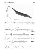
<b>Random walk</b>
0 5 10 15 20 25 30 35 40 45 50
</div>
<span class='text_page_counter'>(11)</span><div class='page_container' data-page=11>
<b>Stationarity</b>
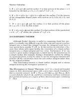
<b>Example: MA(1) process (Moving Average):</b>
Xt = Wt + θWt−1, {Wt} ∼ W N(0, σ2).
We have E[Xt] = 0, and
γ<sub>X</sub>(t + h, t) = E(Xt+hXt)
= E[(Wt+h + θWt+h−1)(Wt + θWt−1)]
=
σ2(1 + θ2) if h = 0,
σ2θ if h = ±1,
0 otherwise.
</div>
<span class='text_page_counter'>(12)</span><div class='page_container' data-page=12>
<b>ACF of the MA(1) process</b>
−100 −8 −6 −4 −2 0 2 4 6 8 10
0.2
0.4
0.6
0.8
1
θ/(1+θ2)
MA(1): X
</div>
<span class='text_page_counter'>(13)</span><div class='page_container' data-page=13>
<b>Stationarity</b>
<b>Example: AR(1) process (AutoRegressive):</b>
Xt = φXt−1 + Wt, {Wt} ∼ W N(0, σ2).
Assume that Xt is stationary and |φ| < 1. Then we have
E[Xt] = φEXt−1
= 0 (from stationarity)
E[X<sub>t</sub>2] = φ2E[X<sub>t</sub>2<sub>−</sub>1] + σ
2
= σ
2
</div>
<span class='text_page_counter'>(14)</span><div class='page_container' data-page=14>
<b>Stationarity</b>
<b>Example: AR(1) process,</b> Xt = φXt−1 + Wt, {Wt} ∼ W N(0, σ2).
Assume that Xt is stationary and |φ| < 1. Then we have
E[Xt] = 0, E[X<sub>t</sub>2] =
σ2
1 − φ2
γX(h) = Cov(φXt+h−1 + Wt+h, Xt)
= φCov(Xt+<sub>h</sub><sub>−</sub>1, X<sub>t</sub>)
= φγX(h − 1)
= φ|h|γX(0) (check for h > 0 and h < 0)
= φ
|h|<sub>σ</sub>2
</div>
<span class='text_page_counter'>(15)</span><div class='page_container' data-page=15>
<b>ACF of the AR(1) process</b>
−100 −8 −6 −4 −2 0 2 4 6 8 10
0.1
0.2
0.3
0.4
0.5
0.6
0.7
0.8
0.9
1
φ|h|
AR(1): X
</div>
<span class='text_page_counter'>(16)</span><div class='page_container' data-page=16>
<b>Linear Processes</b>
An important class of stationary time series:
Xt = µ +
∞
X
j=<sub>−∞</sub>
ψjWt−j
where {Wt} ∼ W N(0, σ<sub>w</sub>2 )
and µ, ψ<sub>j</sub> are parameters satisfying
∞
X
j=<sub>−∞</sub>
</div>
<span class='text_page_counter'>(17)</span><div class='page_container' data-page=17>
<b>Linear Processes</b>
Xt = µ +
∞
X
j=<sub>−∞</sub>
ψjWt−j
We have
µ<sub>X</sub> = µ
γ<sub>X</sub>(h) = σ<sub>w</sub>2
∞
X
j=<sub>−∞</sub>
</div>
<span class='text_page_counter'>(18)</span><div class='page_container' data-page=18>
<b>Examples of Linear Processes: White noise</b>
Xt = µ +
∞
X
j=<sub>−∞</sub>
ψjWt−j
Choose µ,
ψj =
1 if j = 0,
0 otherwise.
</div>
<span class='text_page_counter'>(19)</span><div class='page_container' data-page=19>
<b>Examples of Linear Processes: MA(1)</b>
X<sub>t</sub> = µ +
∞
X
j=<sub>−∞</sub>
ψ<sub>j</sub>W<sub>t</sub><sub>−</sub><sub>j</sub>
Choose µ = 0
ψj =
1 if j = 0,
θ if j = 1,
0 otherwise.
</div>
<span class='text_page_counter'>(20)</span><div class='page_container' data-page=20>
<b>Examples of Linear Processes: AR(1)</b>
X<sub>t</sub> = µ +
∞
X
j=<sub>−∞</sub>
ψ<sub>j</sub>W<sub>t</sub><sub>−</sub><sub>j</sub>
Choose µ = 0
ψj =
φj if j ≥ 0,
0 otherwise.
</div>
<span class='text_page_counter'>(21)</span><div class='page_container' data-page=21>
<b>Estimating the ACF: Sample ACF</b>
Recall: Suppose that {Xt} is a stationary time series.
<b>Its mean is</b>
µ = E[Xt].
<b>Its autocovariance function is</b>
γ(h) = Cov(Xt+h, Xt)
= E[(Xt+h − µ)(Xt − µ)].
<b>Its autocorrelation function is</b>
ρ(h) = γ(h)
</div>
<span class='text_page_counter'>(22)</span><div class='page_container' data-page=22>
<b>Estimating the ACF: Sample ACF</b>
For observations x1, . . . , xn of a time series,
<b>the sample mean is</b> x¯ = 1
n
n
X
t=1
xt.
<b>The sample autocovariance function is</b>
ˆ
γ(h) = 1
n
n−|h|
X
t=1
(x<sub>t</sub>+<sub>|</sub><sub>h</sub><sub>|</sub> −x)(x¯ t −x),¯ for −n < h < n.
<b>The sample autocorrelation function is</b>
ˆ
ρ(h) = γˆ(h)
ˆ
</div>
<span class='text_page_counter'>(23)</span><div class='page_container' data-page=23>
<b>Estimating the ACF: Sample ACF</b>
Sample autocovariance function:
ˆ
γ(h) = 1
n
n−|h|
X
t=1
(xt+<sub>|</sub>h| − x)(x¯ t − x).¯
≈ the sample covariance of (x1, xh+1), . . . ,(xn−h, xn), except that
• we normalize by n instead of n − h, and
</div>
<span class='text_page_counter'>(24)</span><div class='page_container' data-page=24>
<b>Introduction to Time Series Analysis. Lecture 2.</b>
1. Stationarity
2. Autocovariance, autocorrelation
3. MA, AR, linear processes
</div>
<!--links-->