Bài tập chương 2 - Phần 3
Bạn đang xem bản rút gọn của tài liệu. Xem và tải ngay bản đầy đủ của tài liệu tại đây (140.14 KB, 3 trang )
<span class='text_page_counter'>(1)</span><div class='page_container' data-page=1>
242 Chapter 5 Reduction of Multiple Subsystems
<i>R(s) </i>
<i>G(s) </i> <i>R(s)G(s) </i>
<i>R(s) </i>
<i>Vfi </i>
<i>R(s) </i>
<i>G(s) </i>
<i>G(s) </i>
<i>R(s)G(s) </i>
<i>R(s) </i>
1
<i>G{s) </i>
<i>R(s) </i>
FIGURE 5.8 Block diagram
algebra for pickoff p o i n t s
-equivalent forms for moving a
block a. to the left past a
pickoff point; b. to the right
past a pickoff point
<i><b>m </b></i>
<i>R(s)G(s) </i>
<i>G(s) </i>
<i>R(s)G(s) R(s) </i>
<i>R(s)G(s) </i>
<i>R(-i) </i>
<i>G(s) </i>
<i>G(s) </i>
<i>G(s) </i>
<i>R(s)G(s) </i>
<i>R(s)G(s) </i>
<i>R(s)G(s) </i>
along with the forms studied earlier in this section, can be used to reduce a block
diagram to a single transfer function. In each case of Figures 5.7 and 5.8, the
equivalence can be verified by tracing the signals at the input through to the output
and recognizing that the output signals are identical. For example, in Figure 5.7(a),
<i>signals R(s) and X(s) are multiplied by G(s) before reaching the output. Hence, both </i>
<i>block diagrams are equivalent, with C(s) = R(s)G(s) ^fX{s)G(s). In Figure 5.7(b), </i>
<i>R(s) is multiplied by G(s) before reaching the output, but X(s) is not. Hence, both </i>
<i>block diagrams in Figure 5.7(b) are equivalent, with C(s) = R(s)G(s) =f X(s). For </i>
pickoff points, similar reasoning yields similar results for the block diagrams of
Figure 5.8(A)<i> and (b). </i>
Let us now put the whole story together with examples of block diagram
reduction.
FIGURE 5.9 Block diagram
for Example 5.1
<b>Example 5.1 </b>
Block Diagram Reduction via Familiar Forms
PROBLEM: Reduce the block diagram shown in Figure 5.9 to a single transfer
function.
<i>R(s) </i>
<i>Gx(s) </i>
<i>—, \ +1 </i>
7 \ _ + / v A _ ,
—T
<i>G2(s) </i>
<i>Hx(s) </i>
<i>H2(s) </i>
<i>H3(s) </i>
</div>
<span class='text_page_counter'>(2)</span><div class='page_container' data-page=2>
5.2 Block Diagrams 243
SOLUTION: We solve the problem by following the steps in Figure 5.10. First, the
three summing junctions can be collapsed into a single summing junction, as shown
in Figure 5.10(a).
<i>Second, recognize that the three feedback functions, Hi(s), H2(s), and H^(s), are </i>
connected in parallel. They are fed from a common signal source, and their outputs are
<i>summed. The equivalent function is Hi(s) — Hi{s) + Hs(s). Also recognize that G2(s) </i>
<i>and G${s) are connected in cascade. Thus, the equivalent transfer function is the </i>
<i>product, G3(s)G2(s). The results of these steps are shown in Figure 5.10(6). </i>
<i>Finally, the feedback system is reduced and multiplied by Gi(s) to yield the </i>
equivalent transfer function shown in Figure 5.10(c).
<i>R(s) </i>
+\ -*»
<i>G2(s) <b>-~ </b></i>
<i>H{(s) </i>
<i>H2(s) </i>
<i>N^s) </i>
G3(5)
<i>C(s) </i>
<i>(a) </i>
<i>R(s) </i>
<i>Gds) </i> <i>Gi(s)G2(.s) </i>
<i>•- BX{A-H&)+H&) </i>
<i>ib) </i>
<i><b>m </b></i>
<i>G3(s)G2(s)G}(s) </i><i>C(s) </i>
<i>1 + G2{s)G2(s)[H{{s) - H2(s) + H3(s)] </i>
<i>C(s) </i>
<i>(c) </i>
FIGURE 5.10 Steps in solving
Example 5.1: a. Collapse
sum-ming junctions; b. form
equi-valent cascaded system in the
forward path and equivalent
parallel system in the feedback
path; c. form equivalent
feed-back system and multiply by
<i>cascaded Gt(s) </i>
<b>Example 5.2 </b>
Block Diagram Reduction by Moving Blocks
PROBLEM: R e d u c e t h e system shown in Figure 5.11 to a single transfer function.
<i>R(s) + , 0 ^ 1 ( 5 ) </i>
<i>Gi(s) </i> W + ,Ov W <i>G2(s) </i>
w±/6vW
V7(J)
<i>V6(s) </i>
<i>lids) </i>
<i>fUs) </i>
<i>O&i </i>
<i><b>as) </b></i>
<b>w </b>
<i>H-sis) </i></div>
<span class='text_page_counter'>(3)</span><div class='page_container' data-page=3>
<b>244 </b> C h a p t e r 5 R e d u c t i o n of Multiple Subsystems
SOLUTION: In this example we make use of the equivalent forms shown in
<i>Figures 5.7 and 5.8. First, move G2(s) to the left past the pickoff point to create </i>
parallel subsystems, and reduce the feedback system consisting of G3<i>(s) and H3(s). </i>
This result is shown in Figure 5.12(A).
<i>Second, reduce the parallel pair consisting of VG2(s) and unity, and push </i>
Gi(s) to the right past the summing junction, creating parallel subsystems in the
feedback. These results are shown in Figure 5.12(6).
<i>Bb}+/r>Mft </i>
<i><b>®m m +/Q, vm. </b></i>
<i><sub>*W </sub></i><i>vm </i>
<i>Hi(s) </i><i>V7{s) </i>
<i>G2{s) </i>
<i>H2(s) </i>
<i>V4(s) </i>
1
<i>G2(s) </i>
<i>+ </i>
<b>i®-</b>
<i>G3(s) </i><i>l+G3(s)H3(s) </i>
<i>C(s) </i>
<i>R</i>
<i>^</i> +/Ov<i> V</i> <i>^ + </i>
<b><gK </b>
<i>Gl(s)G2{5) </i><i>VA(s) </i>
<i>H2(s) </i>
C,(5)
tf,(s)
<i>Gds) </i>+ 1
<i>G3(s) </i>
<i>1 + G3(s)H3(s) </i>
<i>C(s) </i>
<i><b>m </b></i>
<i>R(s) + </i>
<i><S<5—- G](s)G2{s) </i>
<i>V4(s) </i>
<i>H2(s) </i>
<i><b>GM </b></i><b>+#,(*) </b>
<b>U-*i </b>
<i>Gfr) </i><i>\G2(s) )\l + G3{s)H3(s) </i>
<i>C(s) </i>
<i>R(s) </i> G,(i)G2(5)
<i>1 + G2(s)H2(s) + 0,(5)02(5)//,(5) </i>
V4(5)
-+ 1 G3(5) \
G2<i>(5) ){l + G3(s)H3(s)j </i>
C(5)
<i>R(s) </i> G,(5)G3(5)[1 + G2(5)]
[1 + G2(5)tf2(5) + G,(5)G2(5)//,(5)][1 + G3(5)//3(5)]
<i>C(s) </i>
</div>
<!--links-->