Determination of Source Parameters of Simple-shaped Geologic Subsurface Structures from Self-potential Anomalies Using Enhanced Local Wavenumber Method
Bạn đang xem bản rút gọn của tài liệu. Xem và tải ngay bản đầy đủ của tài liệu tại đây (885.63 KB, 13 trang )
<span class='text_page_counter'>(1)</span><div class='page_container' data-page=1>
83
Original article
Determination of Source Parameters of Simple-shaped
Geologic Subsurface Structures from Self-potential Anomalies
Using Enhanced Local Wavenumber Method
Pham Thanh Luan
1*<sub>, Vu Duc Minh</sub>
1<sub>, Erdinc Oksum</sub>
2<i>1<sub>VNU University of Science, Faculty of Physics, 334 Nguyen Trai, Thanh Xuan, Hanoi, Vietnam </sub></i>
<i>2<sub>Süleyman Demirel University, Engineering Faculty, Department of Geophyisical Engineering, </sub></i>
<i> 32260 Isparta, Turkey </i>
Received 24 March 2019
Revised 29 March 2019; Accepted 29 March 2019
<b>Abstract: Simple geometry model structures can be useful in quantitative evaluation of </b>
self-potential data. In this paper, we solve local wavenumber equation to estimate the horizontal
position, the depth and the type of the causative source geometry by using a linear least-squares
approximation. The advantages of the algorithm in determining the horizontal position and depth
measure are its independency to shape factor of the sources and also its simple computations. The
algorithm is built in Matlab environment. The validity of the algorithm is illustrated on variable
noise-free and random noise included synthetic data from two-dimensional (2-D) models where
the achieved parametric quantities coincide well with the actual ones. The algorithm is also
utilized to real self-potential data from Ergani Copper district, Turkey. The results from the actual
data application are in good agreement with the published literature for the study area. The source
code of the algorithm is available from the authors on request.
<i>Keywords: Local wavenumber, Self-potential, a linear least-squares approximation, Ergani </i>
copper field.
<b>1. Introduction</b>
The self-potential (SP) method, a widely used exploration method in geophysics, is one of the
oldest techniques of geophysics [1, 2]. The method is based on measuring naturally occurring
________
<sub>Corresponding author. </sub>
<i> E-mail address: </i>
</div>
<span class='text_page_counter'>(2)</span><div class='page_container' data-page=2>
electrical potentials in the underground, caused by various physical and chemical mechanisms such as
thermoelectric coupling, electro-kinetic coupling and electrochemical effects [3-5]. Many techniques
have been proposed for the quantitative interpretation of the SP anomaly data. These techniques can be
classified into four categories.
The first category includes the nomograms [6, 7], characteristic curves [8, 9], the analytic signal
(AS) approach [10-12], the depth-curves method [13, 14]. In these methods, the nature of the source
geometry is required to be assumed. In this case, simple geometrical shapes such as spheres, cylinders
and sheet-like sources are used to approximate the buried geological structure. In second category,
Patella (1997) developed a probabilistic tomographic approach [15, 16]. However, his approach is
only available for monopoles charge accumulation in the subsurface whereas natural phenomena, like
oxido-reduction processes or hydroelectric, tend to generate dipolar sources. Revil et al (2001) and
Iuliano et al (2002) extended below the work of Patella (1997) to the case of dipolar sources ([17],
[18]). However, it is noteworthy to mention that the above methods do not contribute to the knowledge
about the source geometry. Another category involves the SP data inversion methods [19-24] where
assumptions of an inert electrode model are being attempted [25]. In these methods, the redox
gradient, the host medium resistivity, and the resistance of electrode are the main critical
considerations on conditioning the gain of the SP anomaly whereas the covering layers, bedrock in
homogeneities, or irregular topography are being secondary factors defining the shape of the anomaly
[23, 26]. Hereby, the requirement of a background resistivity model which is assumed and used to
carry out the inversion procedure is a disadvantage in these methods. The fourth category is naturally
inspired meta-heuristic algorithms that are based on stochastic algorithms. In general, they can be
classified in the three chapters: genetic algorithm [5, 27], simulated annealing [1, 5, 28] and particle
swarm optimization [2, 5, 29-32]. These algorithms only require wider search space bound which is
their major superiority. These algorithms try to find the optimum solution among all possible solutions
that exist in model space and they can avoid local minima without requiring a well-constructed initial
model.
Salem et al (2005) proposed a method based on the enhanced local wavenumber (ELW) for
estimating the horizontal location and the depth of 2D magnetic sources [33]. The advantage of this
method is that it does not assume the geometry of the causative body. Further, their method is efficient
to provide information of the shape of the body once the depth and the origin along the observation
line have been determined. Based on the ELW procedure, Srivastava and Agarwal (2009) developed a
model-independent technique for evaluate SP anomalies [34]. The technique is applicable to 2D
sources that are approximated by a sphere, an inclined sheet, a horizontal cylinder, a dyke, etc.
However, these studies lack detailed description about solution of local wavenumber equations,
making it challenging for readers to understand how some source parameters were determined.
In the present paper, we solve local wavenumber equation with a more detailed mathematical
description for determination of the origin along the observation profile, the depth and the shape type
of the causative body. The applicability of the proposed algorithm has been illustrated through two
synthetic data cases as well as through real SP data from Ergani Copper district, Turkey.
<b>2. Theory </b>
The phase angle [35] is defined as
θ = atan (∂M/ ∂z
∂M/ ∂x)
</div>
<span class='text_page_counter'>(3)</span><div class='page_container' data-page=3>
where M is the field and ∂M/ ∂x and ∂M/ ∂z are the derivatives with respect to horizontal and vertical
directions, respectively.
The measure of changes of the phase angle θ with respect to the horizontal and vertical directions
are known as “local wavenumbers” and are given by [33] as follows
kx=
∂θ
∂x=
1
|AS|2(
∂2M
∂x ∂z
∂M
∂x −
∂2M
∂x2
∂M
∂z)
(2)
kz=
∂θ
∂z=
1
|AS|2(
∂2M
∂x ∂z
∂M
∂z −
∂2M
∂z2
∂M
∂x)
(3)
where
|AS| = √(∂M
∂x)
2
+ (∂M
∂z)
2
(4)
is the AS of the self-potential field, also called the total gradient. Horizontal derivative in equations 2,
3 and 4 can be easily estimated in the space domain using a simple finite-difference method and
discrete measurements of M(x), whereas the vertical derivation is determined in the frequency
domain, as follows [36]
∂M
∂x ≈
Mi+1− Mi−1
2∆x (5)
∂M
∂z ≈ F
−1<sub>[|k|F[M]] </sub> <sub>(6) </sub>
where i represents the discrete measurement of M(x) along the profile at uniform sample interval ∆x,
F[] and F−1[] denotes the Fourier and inverse Fourier transforms, respectively, and k is the
wavenumber.
The local wavenumbers over a few simple geometrical shaped bodies, with horizontal location xo
and depth zo, is given by [33]
kx=
−(N + 1)(z − zo)
(x − xo)2+ (z − zo)2
(7)
kz =
(N + 1)(x − xo)
(x − xo)2+ (z − zo)2
(8)
where x and z are the positions of the observation points, N is a factor related roughly to the geometry
of the buried structure. The shape factor for a sphere, a horizontal cylinder, and a semi infinite vertical
cylinder are 1.5, 1.0 and 0.5, respectively.
Dividing equation 7 by 8, we obtain
kx
kz
= z − zo
x − xo
or
</div>
<span class='text_page_counter'>(4)</span><div class='page_container' data-page=4>
To solve the linear Equation 9, we use a progressively moving window of n data points, and assign
the local wavenumbers kx and kz for variable values of x and z within the window which its center is
positioned to the peak of the amplitude of the AS. As an advantage, the linear Equation 9 does not
need initial knowledge about the shape factor of the source, and can be solved for the depth and
horizontal position of the causative body using least-squares method. The method defines the estimate
of xo and zo the values which minimize the sum of the squares:
S = ∑[kx(i)xo+ kz(i)zo− kx(i)x(i) − kz(i)z]2
n
i=1
(10)
Note that S is a function of parameters xo and zo. We need to find these parameters such that S is
minimum. The necessary condition for S to be minimum is given by [37]
∂S
∂xo
= 0, ∂S
∂zo
= 0 (11)
We may rewrite these equations as
{
∑ kx2(i)xo+ ∑ kx(i)kz(i)zo= ∑ kx2(i)x(i)
n
i=1
n
i=1
n
i=1
+ ∑ kx(i)kz(i)z
n
i=1
∑ kx(i)kz(i)xo+ ∑ kz2(i)zo= ∑ kx(i)kz(i)x(i) + ∑ kz2(i)z
n
i=1
n
i=1
n
i=1
n
i=1
(12)
We have obtained that the values of xo and zo which minimize S satisfy the following matrix
equation
AX = B (13)
where
X = [x<sub>z</sub>o
o],
A =
[
∑ kx2(i)
n
i=1
∑ kx(i)kz(i)
n
i=1
∑ kx(i)kz(i)
n
i=1
∑ kz2(i)
n
i=1 ]
,
B =
[
∑ kx2(i)
n
i=1
x(i) ∑ kx(i)kz(i)z
n
i=1
∑ kx(i)kz(i)
n
i=1
x(i) ∑ kz2(i)
n
i=1
z
]
</div>
<span class='text_page_counter'>(5)</span><div class='page_container' data-page=5>
window comprising a proper length of the data is selected for estimation of the location and depth of
the causative source.
Once the horizontal and vertical positon of the source is calculated from Equation 13, a value for
the shape factor N can be computed from Equations 7 or 8 as the value which minimizes the sum of
the squares:
S′= ∑[kx(i)(x(i) − xo)2+ (z − zo)2− (N + 1)zo]2
n
i=1
(14)
Taking the derivative of S’ with respect to N and setting it to zero gives the following of equation:
∑[kx(i)(x(i) − xo)2+ (z − zo)2] − n(N + 1)zo= 0
n
i=1
(15)
Thus the shape factor N is determined by
N =∑ [kx(i)(x(i) − xo)
2<sub>+ (z − z</sub>
o)2]
n
i=1
nzo
− 1 (16)
<b>3. Application </b>
<i>3.1. Synthetic example </i>
We test the efficiency of the algorithm for various test cases including different theoretical SP
anomalies of a horizontal cylinder and a sphere produced by using depths varied from 5 to 15 m with 1
m increments. The initial anomalies of these models have been generated using the following Equation
[6, 34, 38, 39]:
V(x) = K(x − xo)cosα + zosinα
[(x − xo)2+ zo2]N
(17)
Here, x is the observation point along x-axis, xo is origin of the anomaly, zo is the depth of the
causative source, α is the polarization angle, K is the electric current dipole moment, and N is the
shape factor.
Table 1. Parameters of the model.
Model <i>x mo</i>( ) <i>z mo</i>( ) <i>K mV</i>( ) ( ) N
Sphere 60 varying from 5 to 15 -2000 30 1.5
Cylinder 40 varying from 5 to 15 -2000 30 1
</div>
<span class='text_page_counter'>(6)</span><div class='page_container' data-page=6>
due to the computations of second-order vertical derivative. So it is better to estimate the shape factor
by local wave numbers kx. Figure 2 shows analysis results of the SP anomalies over the horizontal
cylinder source for varying depths. The analysis results are listed in Table 2.
</div>
<span class='text_page_counter'>(7)</span><div class='page_container' data-page=7>
Figure 2a displays a plot of the calculated depths from Equation 13 versus actual depths. To help
in the visualization of the quality of analysis results, a line with zero error was superimposed on Figure
2a. It can be observed from this figure that the result coincide well with the actual depths. A plot of
horizontal locations computed from Equation 13 versus actual depths is illustrated in Figure 2b along
with its comparable average value that is displayed by a straight continuous line. Clearly, the results of
the horizontal location obtained by using Equation 13 are in good agreement with theoretical model.
Figure 2c shows a plot of the shape factor computed from the local wavenumber versus actual depth.
Here, the average line is also shown by continuous line. The obtained results are also in good
agreement with the shape factor of causative body.
Figure 2. Graphical illustration of actual depth versus (a) Computed depth, (b) Computed horizontal location; (c)
Computed shape factor. Horizontal lines represent the average lines of the plotted data in Figure 2b and c.
Table 2. Numerical results in comparison with actual parameters of SP anomaly caused by a cylinder model.
Depth (m) Horizontal
location (m)
Shape
factor
Actual Calculated
5 5.20 40.00 1.04
6 6.17 40.00 1.02
7 7.13 40.00 1.01
8 8.11 40.01 1.01
9 9.08 40.02 1.00
10 10.07 40.04 1.00
11 11.05 40.05 1.00
12 12.04 40.07 0.99
13 13.03 40.10 0.99
14 14.03 40.12 0.99
15 15.02 40.15 1.00
Average 40.05 1.00
Actual 40.00 1.00
</div>
<span class='text_page_counter'>(8)</span><div class='page_container' data-page=8>
of source parameters. Using upward continuation of the anomaly data, the effect of the noise can be
reduced [40, 41].
</div>
<span class='text_page_counter'>(9)</span><div class='page_container' data-page=9>
Figure 4. Graphical illustration of actual depth versus (a) Computed depth; (b) Computed horizontal location; (c)
Computed shape factor. Horizontal lines represent the average lines of the plotted data in Figure 4b and c.
Table 3. Numerical results in comparison with actual parameters of SP anomaly with 10% random noise caused
by a sphere model.
Depth (m) Horizontal
location (m)
Shape
factor
Actual Calculated
5 4.77 60.56 1.40
6 5.72 60.58 1.41
7 6.73 60.61 1.41
8 7.84 60.65 1.43
9 8.92 60.65 1.46
10 9.75 60.70 1.44
11 10.71 60.66 1.43
12 11.72 60.71 1.44
13 13.18 60.71 1.52
14 13.71 60.67 1.44
15 15.37 60.49 1.53
Average 60.64 1.45
Actual 60.00 1.5
</div>
<span class='text_page_counter'>(10)</span><div class='page_container' data-page=10>
<i>3.2. Real data example </i>
</div>
<span class='text_page_counter'>(11)</span><div class='page_container' data-page=11>
In order to demonstrate and assess the applicability of the algorithm, the SP anomaly profile from
Ergani Copper district [34] which was previously interpreted by many authors with different methods
[2, 5, 6, 11, 21, 34, 39, 42] has been analyzed. Figure 5a shows the SP anomaly of the studied area.
For our analysis, the SP anomaly profile of 190 m length was digitized after [34] at intervals of 2 m.
The observed data represents SP anomaly varies from positive (maximum amplitude of about 115 mV)
to negative (maximum amplitude of about 230 mV) values along the SP profile. As a pre-process of
the data, the original field anomaly were upward continued to 2 m to reduce the noise. We have
calculated the AS amplitude (Figure 5b) of data in Figure 5a for proper selection of window position
and its length. The local wavenumber fields are shown in Figure 5c and d respectively. By using
Equation 13, we find two source parameters as: the depth of the body center is at 30.21 m and the
distance from the origin 62.52 m. It is clear that both the depth and location values provided by the
algorithm are found to agree well with results provided by other authors as summarized in Table 4.
The shape factor estimated as a close value to 1 indicates a horizontal cylinder for the geometry of the
source. The result of the shape factor compares favorably with those obtained by recent studies [2, 5,
21, 34, 39, 42] (Table 4).
Table 4. Comparison of the results of this study with the results of previous works available
for the SP data from Ergani, Turkey.
References Horizontal location (m) Depth (m) Structural Index N
[42] - 38.78 1.36
[21] - 35.9 1a
[34] 64.1 28.9 1
[2] 62.3 32.53 -
[5] 79.09 33.59 1.18
[39] - 30.05 -
This study 62.52 30.21 0.97
a<sub> The assumed shape factor. </sub>
<b>4. Conclusion </b>
We have presented solution of local wavenumber equation to estimate the depth and horizontal
position of causative sources without an initial assumption about the geometry of the source. The
geometry of the source is defined by the shape factor which is derived from the computed origin and
depth. The algorithm has been proved on noise-free and noise included synthetic SP anomaly data, and
also applied to real data from Ergani Copper district, Turkey. Test results from synthetic models
provided very close parameters to the real source construction. In the case of the real data example, the
estimated source parameters are found in a good correlation with the previous works.
<b>References </b>
[1] M. Tlas, J. Asfahani, Using of the adaptive simulated annealing (ASA) for quantitative interpretation of
self-potential anomalies due to simple geometrical structures, JKAU: Earth Sci, 19 (2008), 99–118.
[2] E. Pekşen, T. Yas, A.Y. Kayman, C. Özkan C, Application of particle swarm optimization on self-potential data,
Journal of Applied Geophysics, 75(2011), 305–318.
</div>
<span class='text_page_counter'>(12)</span><div class='page_container' data-page=12>
[4] H.M. El-Araby, A new method for complete quantitative interpretation of self-potential anomalies, Journal of
Applied Geophysics, 55 (2004), 211–224, 2004.
[5] G. Göktürkler, C. Balkaya, Inversion of self-potential anomalies caused by simple-geometry bodies using global
optimization algorithms, Journal of Geophysics and Engineering, 9(2012), 498–507.
[6] B.B. Bhattacharya, N. Roy, A note on the use of a nomogram for self-potential anomalies, Geophysical
Prospecting, 29 (1981), 102–104.
[7] B.V.S. Murty, P. Haricharan, Nomogram for the complete interpretation of spontaneous polarization profiles and
sheet like and cylindrical two-dimensional sources, Geophysics, 50 (1985), 1127–1135.
[8] B.S.R. Rao, I.V.R. Murthy, S.J. Reddy, Interpretation of self-potential anomalies of some geometric bodies, Pure
and Applied Geophysics, 78(1970), 66–77.
[9] A.D. Rao, H.V. Ram Babu, Quantitative interpretation of self-potential anomalies due to two-dimensional sheet
like bodies, Geophysics, 48(1983), 1659–1664.
[10] B.N.P Agarwal, Quantitative interpretation of self-potential anomalies, Extended Abstract of the 54th SEG
Annual Meeting and Exposition, Atlanta, (1984) 154–157.
[11] N. Sundarajan, Y. Srinivas, A modified Hilbert transform and its application to self-potential interpretation,
Journal of Applied Geophysics, 36(1996), 137–143.
[12] N. Sundarajan, R.P Srinivasa, V. Sunitha, An analytical method to interpret self-potential anomalies caused by
2-D inclined sheet, Geophysics, 63(1998), 1151–1155.
[13] E.M. Abdelrahman, H.M. El-Araby, T.M. El-Araby, K.S. Essa, A new approach to depth determination from
magnetic anomalies, Geophysics, 67(2002), 1524–1531.
[14] E.M. Abdelrahman, E.R. Abo-Ezz, T.M. El-Araby, K.S. Essa KS, A simple method for depth determination from
self-potential anomalies due to two superimposed structures, Exploration Geophysics, (2015),
doi:10.1071/eg15012.
[15] D. Patella, Introduction to ground surface self-potential tomography, Geophysical Prospecting, 45(1997), 653–
681.
[16] D. Patella, Self-potential global tomography including topographic effects, Geophysical Prospecting, 45(1997),
843–863.
[17] A. Revil, L. Ehouarne, E. Thyreault, Tomography of self-potential anomalies of electrochemical nature,
Geophysical Research Letters, 28(2001), 4363–4366.
[18] T. Iuliano, P. Mauriello, D. Patella, Looking inside Mount Vesuvius by potential fields integrated probability
tomographies, Journal of Volcanology and Geothermal Research, 113(2002), 363–378.
[19] A. Jardani, A. Revil, A. Boleve, A. Crespy, J.P. Dupont, W. Barrash, Tomography of the Darcy velocity from
self-potential measurements, Geophysical Research Letters, 34(2007), L24403.
[20] B.J. Minsley, J. Sogade, F.D. Morgan, Three-dimensional source inversion of self-potential data, Journal of
Geophysical Research, 112(2007), B02202, doi:10.1029/2006JB004262.
[21] K. Essa, S. Mehanee, P.D. Smith, A new inversion algorithm for estimating the best fitting parameters of some
geometrically simple body to measured self-potential anomalies, Exploration Geophysics, 39(2008), 155.
[22] J. Castermant, C.A. Mendonỗa, A. Revil, F. Trolard, G. Bourrié, N. Linde, Redox potential distribution inferred
from self-potential measurements during the corrosion of a burden metallic body, Geophysical Prospecting,
56(2008), 269–282.
[23] C.A. Mendonỗa, Forward and inverse self-potential modeling in mineral exploration, Geophysics, 73(2008),
F33–F43.
[24] A. Soueid-Ahmed, A. Jardani, A. Revil, J.P. Dupont, SP2DINV: A 2D forward and inverse code for streaming
potential problems, Computers & Geosciences, 59(2013), 9–16.
[25] J. Stoll, J. Bigalke, E.W. Grabner, Electrochemical modelling of self-potential anomalies, Surveys in Geophysics,
16(1995), 107–120.
[26] S.S. Vasconcelos, C.A. Mendonỗa, N. Silva, Self-potential signals from pumping tests in laboratory experiments,
Geophysics, 79(2014), EN125–EN133, 2014.
</div>
<span class='text_page_counter'>(13)</span><div class='page_container' data-page=13>
[28] S. Kirkpatrick, C.D. Gelatt, M.P. Vecchi, Optimization by Simulated Annealing, Science, 220(1983), 671–680.
[29] J. Kennedy, R.C. Eberhart, Particle swarm optimization”. Proceedings of the IEEE International Conference on
Neural Networks, (1995), 1942–1948.
[30] J.L. Fernandez-Martinez, E. Garcia-Gonzalo, J.P. Fernandez-Alvarez, H.A. Kuzma, C.O. Menendez Perez, PSO:
a powerful algorithm to solve geophysical inverse problems: application to a 1D-DC resistivity case, Journal of
Applied Geophysics, 71(2010), 13–25.
[31] J.L. Fernandez-Martinez, E. Garcia-Gonzalo, V. Naudet, Particle swarm optimization applied to solving and
appraising the streaming-potential inverse problem, Geophysics, 75(2010), WA3–WA15.
[32] E. Momeni, D.J. Armaghani, M. Hajihassani, M.F.M. Amin, Prediction of uniaxial compressive strength of rock
samples using hybrid particle swarm optimization-based artificial neural networks, Measurement, 60(2015), 50–
63.
[33] A.Salem, D. Ravat, R. Smith, K. Ushijima. Interpretation of magnetic data using an enhanced local wave number
(ELW) method, Geophysics, 70(2005), L7–12.
[34] S. Srivastava, B.N.P. Agarwal, Interpretation of self-potential anomalies by Enhanced Local Wave number
technique, Journal of Applied Geophysics, 68(2009), 259–268, 2009.
[35] J.B. Thurston, R.S. Smith, Automatic conversion of magnetic data to depth, dip, and susceptibility contrast using
the SPI(TM) method, Geophysics, 62(1997), 807–813.
[36] R.J. Blakely, Potential Theory in Gravity and Magnetic Applications. Cambridge, Cambridge University Press,
1995
[37] S.J. Miller, The method of least squares, Mathematics Department Brown University, (2006), 1–7.
[38] V. Srivardhan, S.K. Pal, J. Vaish, S. Kumar, A.K. Bharti, P. Priyam, Particle swarm optimization inversion of
self-potential data for depth estimation of coal fires over East Basuria colliery, Jharia coalfield, India, Environ
Earth Sci 75(2016), 688.
[39] R. Di Maio, e. Piegari, P. Rani, Source depth estimation of self-potential anomalies by spectral methods, Journal
of Applied Geophysics, 136 (2017), 315–325.
[40] L.T. Pham, E. Oksum, T.D. Do, M. Le-Huy, New method for edges detection of magnetic sources using logistic
function, Geofizicheskiy Zhurnal, 40(2018), 127-135.
[41] L.T. Pham, E. Oksum, T.D. Do, Edge enhancement of potential field data using the logistic function and the total
horizontal gradient, Acta Geodaetica et Geophysica, 54(2019), pp. 143-155.
</div>
<!--links-->