DSA First Draft

Bạn đang xem bản rút gọn của tài liệu. Xem và tải ngay bản đầy đủ của tài liệu tại đây (966.53 KB, 97 trang )

(1)<div class='page_container' data-page=1>

DSA

D a t a S t r u c t u r e s a n d A l g o r i t h m s

Annotated Reference with Examples

</div>
(2)<div class='page_container' data-page=2>

Annotated Reference with Examples

First Edition

</div>
(3)<div class='page_container' data-page=3>

This book is made exclusively available from DotNetSlackers

</div>
(4)<div class='page_container' data-page=4>

Thank you for viewing the first preview of our book. As you might have
guessed there are many parts of the book that are still partially complete, or
not started.

The following list shows the chapters that are partially completed:

1. Balanced Trees

2. Sorting

3. Numeric

4. Searching

5. Sets

6. Strings

While at this moment in time we don’t acknowledge any of those who have

helped us thus far, we would like to thank Jon Skeet who has helped with some
of the editing. It would be wise to point out that the vast majority of this book
has not been edited yet. The next preview will be a more toned version.

</div>
(5)<div class='page_container' data-page=5>

1 Introduction 1

1.1 What this book is, and what it isn’t . . . 1

1.2 Assumed knowledge . . . 1

1.2.1 Big Oh notation . . . 1

1.2.2 Imperative programming language . . . 3

1.2.3 Object oriented concepts . . . 4

1.3 Pseudocode . . . 4

1.4 Tips for working through the examples . . . 6

1.5 Book outline . . . 6

1.6 Where can I get the code? . . . 7

1.7 Final messages . . . 7

I

Data Structures

8

2 Linked Lists 9

2.1 Singly Linked List . . . 9

2.1.1 Insertion . . . 10

2.1.2 Searching . . . 10

2.1.3 Deletion . . . 11

2.1.4 Traversing the list . . . 12

2.1.5 Traversing the list in reverse order . . . 13

2.2 Doubly Linked List . . . 13

2.2.1 Insertion . . . 15

2.2.2 Deletion . . . 15

2.2.3 Reverse Traversal . . . 16

2.3 Summary . . . 17

3 Binary Search Tree 18
3.1 Insertion . . . 19

3.2 Searching . . . 20

3.3 Deletion . . . 21

3.4 Finding the parent of a given node . . . 23

3.5 Attaining a reference to a node . . . 23

3.6 Finding the smallest and largest values in the binary search tree 24
3.7 Tree Traversals . . . 25

3.7.1 Preorder . . . 25

3.7.2 Postorder . . . 25

</div>
(6)<div class='page_container' data-page=6>

3.8 Summary . . . 30

4 Heap 31
4.1 Insertion . . . 32

4.2 Deletion . . . 36

4.3 Searching . . . 37

4.4 Traversal . . . 40

4.5 Summary . . . 41

5 Sets 42
5.1 Unordered . . . 44

5.1.1 Insertion . . . 44

5.2 Ordered . . . 45

5.3 Summary . . . 45

6 Queues 46
6.1 Standard Queue . . . 47

6.2 Priority Queue . . . 47

6.3 Summary . . . 47

7 Balanced Trees 50
7.1 AVL Tree . . . 50

II

Algorithms

51

8 Sorting 52
8.1 Bubble Sort . . . 52

8.2 Merge Sort . . . 52

8.3 Quick Sort . . . 54

8.4 Insertion Sort . . . 56

8.5 Shell Sort . . . 57

8.6 Radix Sort . . . 57

8.7 Summary . . . 59

9 Numeric 61
9.1 Primality Test . . . 61

9.2 Base conversions . . . 61

9.3 Attaining the greatest common denominator of two numbers . . 62

9.4 Computing the maximum value for a number of a specific base
consisting of N digits . . . 63

9.5 Factorial of a number . . . 63

10 Searching 65
10.1 Sequential Search . . . 65

10.2 Probability Search . . . 65

11 Sets 67

</div>
(7)<div class='page_container' data-page=7>

12 Strings 68
12.1 Reversing the order of words in a sentence . . . 68

12.2 Detecting a palindrome . . . 69

12.3 Counting the number of words in a string . . . 70

12.4 Determining the number of repeated words within a string . . . . 72

12.5 Determining the first matching character between two strings . . 73

A Algorithm Walkthrough 75

A.1 Iterative algorithms . . . 75

A.2 Recursive Algorithms . . . 77

A.3 Summary . . . 79

B Translation Walkthrough 80

B.1 Summary . . . 81

C Recursive Vs. Iterative Solutions 82
C.1 Activation Records . . . 83

C.2 Some problems are recursive in nature . . . 84

C.3 Summary . . . 84

D Symbol Definitions 86

</div>
(8)<div class='page_container' data-page=8>

Every book has a story as to how it came about and this one is no different,
although we would be lying if we said its development had not been somewhat
impromptu. Put simply this book is the result of a series of emails sent back
and forth between the two authors during the development of a library for
the .NET framework of the same name (with the omission of the subtitle of
course!). The conversation started off something like, “Why don’t we create
a more aesthetically pleasing way to present our pseudocode?” After a few
weeks this new presentation style had in fact grown into pseudocode listings
with chunks of text describing how the data structure or algorithm in question
works and various other things about it. At this point we thought, “What the
heck, let’s make this thing into a book!” And so, in the summer of 2008 we

began work on this book side by side with the actual library implementation.

When we started writing this book the only things that we were sure about
with respect to how the book should be structured were:

1. always make explanations as simple as possible while maintaining a
moder-ately fine degree of precision to keep the more eager minded reader happy;
and

2. inject diagrams to demystify problems that are even moderatly challenging
to visualise (. . . and so we could remember how our own algorithms worked
when looking back at them!); and finally

3. present concise and self-explanatory pseudocode listings that can be ported
easily to most mainstream imperative programming languages like C++,
C#, and Java.

A key factor of this book and its associated implementations is that all
algorithms (unless otherwise stated) were designed by us, using the theory of
the algorithm in question as a guideline (for which we are eternally grateful to
their original creators). Therefore they may sometimes turn out to be worse
than the “normal” implementations—and sometimes not. We are two fellows
of the opinion that choice is a great thing. Read our book, read several others
on the same subject and use what you see fit from each (if anything) when
implementing your own version of the algorithms in question.

Through this book we hope that you will see the absolute necessity of
under-standing which data structure or algorithm to use for a certain scenario. In all
projects, especially those that are concerned with performance (here we apply
an even greater emphasis on real-time systems) the selection of the wrong data

structure or algorithm can be the cause of a great deal of performance pain.

</div>
(9)<div class='page_container' data-page=9>

Therefore it is absolutely key that you think about the run time complexity and
space requirements of your selected approach. In this book we only explain the
theoretical implications to consider, but this is for a good reason: compilers are
very different in how they work. One C++ compiler may have some amazing
optimisation phases specifically targeted at recursion, another may not, for
ex-ample. Of course this is just an example but you would be surprised by how
many subtle differences there are between compilers. These differences which
may make a fast algorithm slow, and vice versa. We could also factor in the
same concerns about languages that target virtual machines, leaving all the
actual various implementation issues to you given that you will know your
lan-guage’s compiler much better than us...well in most cases. This has resulted in
a more concise book that focuses on what we think are the key issues.

One final note: never take the words of others as gospel; verify all that can
be feasibly verified and make up your own mind.

We hope you enjoy reading this book as much as we have enjoyed writing it.
Granville Barnett

</div>
(10)<div class='page_container' data-page=10>

Acknowledgements

</div>
(11)<div class='page_container' data-page=11></div>
(12)<div class='page_container' data-page=12>

Introduction

1.1 What this book is, and what it isn’t

This book provides implementations of common and uncommon algorithms in

pseudocode which is language independent and provides for easy porting to most
imperative programming languages. It is not a definitive book on the theory of
data structures and algorithms.

For the most part this book presents implementations devised by the authors
themselves based on the concepts by which the respective algorithms are based
upon so it is more than possible that our implementations differ from those
considered the norm.

You should use this book alongside another on the same subject, but one
that contains formal proofs of the algorithms in question. In this book we use
the abstract big Oh notation to depict the run time complexity of algorithms
so that the book appeals to a larger audience.

1.2 Assumed knowledge

We have written this book with few assumptions of the reader, but some have
been necessary in order to keep the book as concise and approachable as possible.
We assume that the reader is familiar with the following:

1. Big Oh notation

2. An imperative programming language

3. Object oriented concepts

1.2.1 Big Oh notation

For run time complexity analysis we use big Oh notation extensively so it is vital
that you are familiar with the general concepts to determine which is the best

algorithm for you in certain scenarios. We have chosen to use big Oh notation
for a few reasons, the most important of which is that it provides an abstract
measurement by which we can judge the performance of algorithms without
using mathematical proofs.

</div>
(13)<div class='page_container' data-page=13>

CHAPTER 1. INTRODUCTION 2

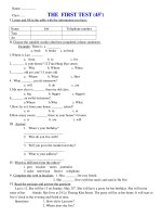
Figure 1.1: Algorithmic run time expansion

Figure 1.1 shows some of the run times to demonstrate how important it is to
choose an efficient algorithm. For the sanity of our graph we have omitted cubic

O(n3), and exponential O(2n) run times. Cubic and exponential algorithms

should only ever be used for very small problems (if ever!); avoid them if feasibly
possible.

The following list explains some of the most common big Oh notations:

O(1) constant: the operation doesn’t depend on the size of its input, e.g. adding
a node to the tail of a linked list where we always maintain a pointer to
the tail node.

O(n) linear: the run time complexity is proportionate to the size of n.

O(log n) logarithmic: normally associated with algorithms that break the problem
into smaller chunks per each invocation, e.g. searching a binary search
tree.

O(n log n) just n log n: usually associated with an algorithm that breaks the problem

into smaller chunks per each invocation, and then takes the results of these
smaller chunks and stitches them back together, e.g. quick sort.

O(n2) quadratic: e.g. bubble sort.

O(n3) cubic: very rare.

O(2n) exponential: incredibly rare.

</div>
(14)<div class='page_container' data-page=14>

and recursive calls—so that you can get the most efficient run times for your
algorithms.

The biggest asset that big Oh notation gives us is that it allows us to
es-sentially discard things like hardware. If you have two sorting algorithms, one
with a quadratic run time, and the other with a logarithmic run time then the
logarithmic algorithm will always be faster than the quadratic one when the
data set becomes suitably large. This applies even if the former is ran on a
ma-chine that is far faster than the latter. Why? Because big Oh notation isolates
a key factor in algorithm analysis: growth. An algorithm with a quadratic run
time grows faster than one with a logarithmic run time. It is generally said at
some point as n → ∞ the logarithmic algorithm will become faster than the
quadratic algorithm.

Big Oh notation also acts as a communication tool. Picture the scene: you
are having a meeting with some fellow developers within your product group.
You are discussing prototype algorithms for node discovery in massive networks.
Several minutes elapse after you and two others have discussed your respective
algorithms and how they work. Does this give you a good idea of how fast each
respective algorithm is? No. The result of such a discussion will tell you more
about the high level algorithm design rather than its efficiency. Replay the scene

back in your head, but this time as well as talking about algorithm design each
respective developer states the asymptotic run time of their algorithm. Using
the latter approach you not only get a good general idea about the algorithm
design, but also key efficiency data which allows you to make better choices
when it comes to selecting an algorithm fit for purpose.

Some readers may actually work in a product group where they are given
budgets per feature. Each feature holds with it a budget that represents its
up-permost time bound. If you save some time in one feature it doesn’t necessarily
give you a buffer for the remaining features. Imagine you are working on an
application, and you are in the team that is developing the routines that will
essentially spin up everything that is required when the application is started.
Everything is great until your boss comes in and tells you that the start up
time should not exceed n ms. The efficiency of every algorithm that is invoked
during start up in this example is absolutely key to a successful product. Even
if you don’t have these budgets you should still strive for optimal solutions.

Taking a quantitative approach for many software development properties
will make you a far superior programmer - measuring one’s work is critical to
success.

1.2.2 Imperative programming language

All examples are given in a pseudo-imperative coding format and so the reader
must know the basics of some imperative mainstream programming language
to port the examples effectively, we have written this book with the following
target languages in mind:

1. C++

2. C#

</div>
(15)<div class='page_container' data-page=15>

CHAPTER 1. INTRODUCTION 4

The reason that we are explicit in this requirement is simple—all our
imple-mentations are based on an imperative thinking style. If you are a functional
programmer you will need to apply various aspects from the functional paradigm
to produce efficient solutions with respect to your functional language whether
it be Haskell, F#, OCaml, etc.

Two of the languages that we have listed (C# and Java) target virtual
machines which provide various things like security sand boxing, and memory
management via garbage collection algorithms. It is trivial to port our
imple-mentations to these languages. When porting to C++ you must remember to
use pointers for certain things. For example, when we describe a linked list
node as having a reference to the next node, this description is in the context
of a managed environment. In C++ you should interpret the reference as a
pointer to the next node and so on. For programmers who have a fair amount
of experience with their respective language these subtleties will present no
is-sue, which is why we really do emphasise that the reader must be comfortable
with at least one imperative language in order to successfully port the
pseudo-implementations in this book.

It is essential that the user is familiar with primitive imperative language
constructs before reading this book otherwise you will just get lost. Some
algo-rithms presented in this book can be confusing to follow even for experienced
programmers!

1.2.3 Object oriented concepts

For the most part this book does not use features that are specific to any one
language. In particular, we never provide data structures or algorithms that
work on generic types—this is in order to make the samples as easy to follow
as possible. However, to appreciate the designs of our data structures you will
need to be familiar with the following object oriented (OO) concepts:

1. Inheritance

2. Encapsulation

3. Polymorphism

This is especially important if you are planning on looking at the C# target
that we have implemented (more on that in §1.6) which makes extensive use
of the OO concepts listed above. As a final note it is also desirable that the
reader is familiar with interfaces as the C# target uses interfaces throughout
the sorting algorithms.

1.3 Pseudocode

Throughout this book we use pseudocode to describe our solutions. For the
most part interpreting the pseudocode is trivial as it looks very much like a
more abstract C++, or C#, but there are a few things to point out:

1. Pre-conditions should always be enforced

</div>
(16)<div class='page_container' data-page=16>

3. The type of parameters is inferred

4. All primitive language constructs are explicitly begun and ended

If an algorithm has a return type it will often be presented in the
post-condition, but where the return type is sufficiently obvious it may be omitted
for the sake of brevity.

Most algorithms in this book require parameters, and because we assign no
explicit type to those parameters the type is inferred from the contexts in which
it is used, and the operations performed upon it. Additionally, the name of
the parameter usually acts as the biggest clue to its type. For instance n is a
pseudo-name for a number and so you can assume unless otherwise stated that

n translates to an integer that has the same number of bits as a WORD on a

32 bit machine, similarly l is a pseudo-name for a list where a list is a resizeable
array (e.g. a vector).

The last major point of reference is that we always explicitly end a language
construct. For instance if we wish to close the scope of a for loop we will
explicitly state end for rather than leaving the interpretation of when scopes
are closed to the reader. While implicit scope closure works well in simple code,
in complex cases it can lead to ambiguity.

The pseudocode style that we use within this book is rather straightforward.
All algorithms start with a simple algorithm signature, e.g.

1) algorithm AlgorithmName(arg1, arg2, ..., argN )
2) ...

n) end AlgorithmName

Immediately after the algorithm signature we list any Pre or Post

condi-tions.

1) algorithm AlgorithmName(n)

2) Pre: n is the value to compute the factorial of

3) n ≥ 0

4) Post: the factorial of n has been computed
5) // ...

n) end AlgorithmName

The example above describes an algorithm by the name of AlgorithmName,
which takes a single numeric parameter n. The pre and post conditions follow
the algorithm signature; you should always enforce the pre-conditions of an
algorithm when porting them to your language of choice.

Normally what is listed as a pre-conidition is critical to the algorithms
opera-tion. This may cover things like the actual parameter not being null, or that the
collection passed in must contain at least n items. The post-condition mainly
describes the effect of the algorithms operation. An example of a post-condition
might be “The list has been sorted in ascending order”

</div>
(17)<div class='page_container' data-page=17>

CHAPTER 1. INTRODUCTION 6

information back to the caller and tell them why the algorithm has failed to be
invoked.

1.4 Tips for working through the examples

As with most books you get out what you put in and so we recommend that in
order to get the most out of this book you work through each algorithm with a
pen and paper to track things like variable names, recursive calls etc.

The best way to work through algorithms is to set up a table, and in that
table give each variable its own column and continuously update these columns.
This will help you keep track of and visualise the mutations that are occurring
throughout the algorithm. Often while working through algorithms in such
a way you can intuitively map relationships between data structures rather
than trying to work out a few values on paper and the rest in your head. We
suggest you put everything on paper irrespective of how trivial some variables
and calculations may be so that you always have a point of reference.

When dealing with recursive algorithm traces we recommend you do the
same as the above, but also have a table that records function calls and who
they return to. This approach is a far cleaner way than drawing out an elaborate
map of function calls with arrows to one another, which gets large quickly and
simply makes things more complex to follow. Track everything in a simple and
systematic way to make your time studying the implementations far easier.

1.5 Book outline

We have split this book into two parts:

Part 1: Provides discussion and pseudo-implementations of common and
uncom-mon data structures; and

Part 2: Provides algorithms of varying purposes from sorting to string operations.
The reader doesn’t have to read the book sequentially from beginning to

end: chapters can be read independently from one another. We suggest that
in part 1 you read each chapter in its entirety, but in part 2 you can get away
with just reading the section of a chapter that describes the algorithm you are
interested in.

</div>
(18)<div class='page_container' data-page=18>

1.6 Where can I get the code?

This book doesn’t provide any code specifically aligned with it, however we do
actively maintain an open source project1that houses a C# implementation of

all the pseudocode listed. The project is named Data Structures and Algorithms
(DSA) and can be found at />

1.7 Final messages

We have just a few final messages to the reader that we hope you digest before
you embark on reading this book:

1. Understand how the algorithm works first in an abstract sense; and

2. Always work through the algorithms on paper to understand how they
achieve their outcome

If you always follow these key points, you will get the most out of this book.

1All readers are encouraged to provide suggestions, feature requests, and bugs so we can

</div>
(19)<div class='page_container' data-page=19>

Part I

Data Structures

</div>
(20)<div class='page_container' data-page=20>

Linked Lists

Linked lists can be thought of from a high level perspective as being a series
of nodes, each node has at least a single pointer to the next node, and in the
last nodes case a null pointer representing that there are no more nodes in the
linked list.

In DSA our implementations of linked lists always maintain head and tail
pointers so that insertion at either the head or tail of the list is constant.
Ran-dom insertion is excluded from this and will be a linear operation, as such the
following are characteristics of linked lists in DSA:

1. Insertion is O(1)

2. Deletion is O(n)

3. Searching is O(n)

Out of the three operations the one that stands out is that of insertion, in
DSA we chose to always maintain pointers (or more aptly references) to the
node(s) at the head and tail of the linked list and so performing a traditional
insertion to either the front or back of the linked list is an O(1) operation. An
exception to this rule is when performing an insertion before a node that is
neither the head nor tail in a singly linked list, that is the node we are inserting
before is somewhere in the middle of the linked list in which case random
inser-tion is O(n). It is apparent that in order to add before the designated node we
need to traverse the linked list to acquire a pointer to the node before the node
we want to insert before which yields an O(n) run time.

These data structure’s are trivial, but they have a few key points which at

times make them very attractive:

1. the list is dynamically resized, thus it incurs no copy penalty like an array
or vector would eventually incur; and

2. insertion is O(1).

2.1 Singly Linked List

Singly linked list’s are one of the most primitive data structures you will find in
this book, each node that makes up a singly linked list consists of a value, and
a reference to the next node (if any) in the list.

</div>
(21)<div class='page_container' data-page=21>

CHAPTER 2. LINKED LISTS 10

Figure 2.1: Singly linked list node

Figure 2.2: A singly linked list populated with integers

2.1.1 Insertion

In general when people talk about insertion with respect to linked lists of any
form they implicitly refer to the adding of a node to the tail of the list, thus
when you use an API like that of DSA and you see a general purpose method
that adds a node to the list assume that you are adding that node to the tail of
the list not the head.

Adding a node to a singly linked list has only two cases:

1. head = ∅ in which case the node we are adding is now both the head and
tail of the list; or

2. we simply need to append our node onto the end of the list updating the

tail reference appropriately.

1) algorithm Add(value)

2) Pre: value is the value to add to the list

3) Post: value has been placed at the tail of the list
4) n ← node(value)

5) if head = ∅

6) head ← n

7) tail ← n

8) else

9) tail.Next ← n

10) tail ← n

11) end if
12) end Add

As an example of the previous algorithm consider adding the following
se-quence of integers to the list: 1, 45, 60, and 12, the resulting list is that of
Figure 2.2.

2.1.2 Searching

</div>
(22)<div class='page_container' data-page=22>

1) algorithm Contains(head, value)

2) Pre: head is the head node in the list
3) value is the value to search for

4) Post: the item is either in the linked list, true; otherwise false

5) n ← head

6) while n 6= ∅ and n.Value 6= value

7) n ← n.Next

8) end while
9) if n = ∅

10) return false
11) end if

12) return true
13) end Contains

2.1.3 Deletion

Deleting a node from a linked list is straight forward but there are a few cases
in which we need to accommodate for:

1. the list is empty; or

2. the node to remove is the only node in the linked list; or

3. we are removing the head node; or

4. we are removing the tail node; or

5. the node to remove is somewhere in between the head and tail; or

6. the item to remove doesn’t exist in the linked list

</div>
(23)<div class='page_container' data-page=23>

CHAPTER 2. LINKED LISTS 12

1) algorithm Remove(head, value)

2) Pre: head is the head node in the list

3) value is the value to remove from the list

4) Post: value is removed from the list, true; otherwise false
5) if head = ∅

6) // case 1
7) return false
8) end if

9) n ← head

10) if n.Value = value

11) if head = tail
12) // case 2

13) head ← ∅

14) tail ← ∅

15) else
16) // case 3

17) head ← head.Next

18) end if
19) return true
20) end if

21) while n.Next 6= ∅ and n.Next.Value 6= value

22) n ← n.Next

23) end while
24) if n.Next 6= ∅
25) if n.Next = tail
26) // case 4

27) tail ← n

28) end if

29) // this is only case 5 if the conditional on line 25) was f f

30) n.Next ← n.Next.Next

31) return true
32) end if

33) // case 6
34) return false
35) end Remove

2.1.4 Traversing the list

Traversing a singly list is the same as that of traversing a doubly linked list
(defined in §2.2), you start at the head of the list and continue until you come
across a node that is ∅. The two cases are as follows:

1. node = ∅, we have exhausted all nodes in the linked list; or

2. we must update the node reference to be node.Next.

The algorithm described is a very simple one that makes use of a simple

</div>
(24)<div class='page_container' data-page=24>

1) algorithm Traverse(head)

2) Pre: head is the head node in the list

3) Post: the items in the list have been traversed

4) n ← head

5) while n 6= 0

6) yield n.Value

7) n ← n.Next

8) end while
9) end Traverse

2.1.5 Traversing the list in reverse order

Traversing a singly linked list in a forward manned is simple (i.e. left to right) as
demonstrated in §2.1.4, however, what if for some reason we wanted to traverse
the nodes in the linked list in reverse order? The algorithm to perform such
a traversal is very simple, and just like demonstrated in §2.1.3 we will need to
acquire a reference to the previous node of a node, even though the fundamental
characteristics of the nodes that make up a singly linked list prohibit this by
design.

The following algorithm being applied to a linked list with the integers 5,
10, 1, and 40 is depicted in Figure 2.3.

1) algorithm ReverseTraversal(head, tail)
2) Pre: head and tail belong to the same list

3) Post: the items in the list have been traversed in reverse order
4) if tail 6= ∅

5) curr ← tail

6) while curr 6= head

7) prev ← head

8) while prev.Next 6= curr

9) prev ← prev.Next

10) end while
11) yield curr.Value

12) curr ← prev

13) end while
14) yield curr.Value
15) end if

16) end ReverseTraversal

This algorithm is only of real interest when we are using singly linked lists, as
you will soon find out doubly linked lists (defined in §2.2) have certain properties
that remove the challenge of reverse list traversal as shown in §2.2.3.

2.2 Doubly Linked List

</div>
(25)<div class='page_container' data-page=25>

CHAPTER 2. LINKED LISTS 14

Figure 2.3: Reverse traveral of a singly linked list

</div>
(26)<div class='page_container' data-page=26>

It would be wise to point out that the following algorithms for the doubly
linked list are exactly the same as those listed previously for the singly linked
list:

1. Searching (defined in §2.1.2)

2. Traversal (defined in §2.1.4)

2.2.1 Insertion

The only major difference between the algorithm in §2.1.1 is that we need to
remember to bind the previous pointer of n to the previous tail node if n was
not the first node to be inserted into the list.

1) algorithm Add(value)

2) Pre: value is the value to add to the list

3) Post: value has been placed at the tail of the list
4) n ← node(value)

5) if head = ∅

6) head ← n

7) tail ← n

8) else

9) n.Previous ← tail

10) tail.Next ← n

11) tail ← n

12) end if
13) end Add

Figure 2.5 shows the doubly linked list after adding the sequence of integers
defined in §2.1.1.

Figure 2.5: Doubly linked list populated with integers

2.2.2 Deletion

</div>
(27)<div class='page_container' data-page=27>

CHAPTER 2. LINKED LISTS 16

1) algorithm Remove(head, value)

2) Pre: head is the head node in the list

3) value is the value to remove from the list

4) Post: value is removed from the list, true; otherwise false
5) if head = ∅

6) return false
7) end if

8) if value = head.Value
9) if head = tail

10) head ← ∅

11) tail ← ∅

12) else

13) head ← head.Next

14) head.Previous ← ∅

15) end if
16) return true
17) end if

18) n ← head.Next

19) while n 6= ∅ and value 6= n.Value

20) n ← n.Next

21) end while
22) if n = tail

23) tail ← tail.Previous

24) tail.Next ← ∅

25) return true
26) else if n 6= ∅

27) n.Previous.Next ← n.Next

28) n.Next.Previous ← n.Previous

29) return true
30) end if

31) return false
32) end Remove

2.2.3 Reverse Traversal

</div>
(28)<div class='page_container' data-page=28>

Figure 2.6: Doubly linked list reverse traversal

1) algorithm ReverseTraversal(tail)

2) Pre: tail is the tail node of the list to traverse
3) Post: the list has been traversed in reverse order
4) n ← tail

5) while n 6= ∅
6) yield n.Value

7) n ← n.Previous

8) end while
9) end ReverseTraversal

2.3 Summary

Linked lists are good to use when you have an unknown amount of items to

store. Using a data structure like an array would require you to be up front
about the size of the array. Were you to exceed that size then you would need
to invoke a resizing algorithm which has a linear run time. You should also use
linked lists when you will only remove nodes at either the head or tail of the list
to maintain a constant run time. This requires constantly maintained pointers
to the nodes at the head and tail of the list but the memory overhead will pay
for itself if this is an operation you will be performing many times.

What linked lists are not very good for is random insertion, accessing nodes
by index, and searching. At the expense of a little memory (in most cases 4
bytes would suffice), and a few more read/writes you could maintain a count
variable that tracks how many items are contained in the list so that accessing
such a primitive property is a constant operation - you just need to update

count during the insertion and deletion algorithms.

</div>
(29)<div class='page_container' data-page=29>

Chapter 3 Binary Search Tree

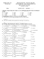
Binary search tree’s (BSTs) are very simple to understand, consider the
follow-ing where by we have a root node n, the left sub tree of n contains values < n,
the right sub tree however contains nodes whose values are ≥ n.

BSTs are of interest because they have operations which are favourably fast,
insertion, look up, and deletion can all be done in O(log n). One of the things
that I would like to point out and address early is that O(log n) times for the
aforementioned operations can only be attained if the BST is relatively balanced
(for a tree data structure with self balancing properties see AVL tree defined in

§7.1).

In the following examples you can assume, unless used as a parameter alias
that root is a reference to the root node of the tree.

14 31

7 17

Figure 3.1: Simple unbalanced binary search tree

</div>
(30)<div class='page_container' data-page=30>

3.1 Insertion

As mentioned previously insertion is an O(log n) operation provided that the
tree is moderately balanced.

1) algorithm Insert(value)

2) Pre: value has passed custom type checks for type T

3) Post: value has been placed in the correct location in the tree
4) if root = ∅

5) root ← node(value)

6) else

7) InsertNode(root, value)
8) end if

9) end Insert

1) algorithm InsertNode(root, value)
2) Pre: root is the node to start from

3) Post: value has been placed in the correct location in the tree
4) if value < root.Value

5) if root.Left = ∅

6) root.Left ← node(value)

7) else

8) InsertNode(root.Left, value)
9) end if

10) else

11) if root.Right = ∅

12) root.Right ← node(value)

13) else

14) InsertNode(root.Right, value)

15) end if

16) end if
17) end InsertNode

</div>
(31)<div class='page_container' data-page=31>

CHAPTER 3. BINARY SEARCH TREE 20

3.2 Searching

Searching a BST is really quite simple, the pseudo code is self explanatory but
we will look briefly at the premise of the algorithm nonetheless.

We have talked previously about insertion, we go either left or right with
the right sub tree containing values that are ≥ n where n is the value of the
node we are inserting, when searching the rules are made a little more atomic
and at any one time we have four cases to consider:

1. the root = ∅ in which case value is not in the BST; or

2. root.Value = value in which case value is in the BST; or

3. value < root.Value, we must inspect the left sub tree of root for value; or

4. value > root.Value, we must inspect the right sub tree of root for value.

1) algorithm Contains(root, value)

2) Pre: root is the root node of the tree, value is what we would like to locate
3) Post: value is either located or not

4) if root = ∅
5) return false
6) end if

7) if root.Value = value
8) return true

9) else if value < root.Value

10) return Contains(root.Left, value)
11) else

12) return Contains(root.Right, value)
13) end if

</div>
(32)<div class='page_container' data-page=32>

3.3 Deletion

Removing a node from a BST is fairly straight forward, there are four cases that
we must consider though:

1. the value to remove is a leaf node; or

2. the value to remove has a right sub tree, but no left sub tree; or

3. the value to remove has a left sub tree, but no right sub tree; or

4. the value to remove has both a left and right sub tree in which case we
promote the largest value in the left sub tree.

There is also an implicitly added fifth case whereby the node to be removed

is the only node in the tree. In this case our current list of cases cover such an
occurrence, but you should be aware of this.

14 31

9
#1: Leaf Node
#2: Right subtree

no left subtree
#3: Left subtree

no right subtree

#4: Right subtree

and left subtree

Figure 3.2: binary search tree deletion cases

The Remove algorithm described later relies on two further helper 
algo-rithms named F indP arent, and F indN ode which are described in §3.4 and

</div>
(33)<div class='page_container' data-page=33>

CHAPTER 3. BINARY SEARCH TREE 22

1) algorithm Remove(value)

2) Pre: value is the value of the node to remove, root is the root node of the BST
3) Post: node with value is removed if found in which case yields true, otherwise false
4) nodeT oRemove ← FindNode(value)

5) if nodeT oRemove = ∅

6) return false // value not in BST
7) end if

8) parent ← FindParent(value)

9) if count = 1 // count keeps track of the # of nodes in the BST
10) root ← ∅ // we are removing the only node in the BST

11) else if nodeT oRemove.Left = ∅ and nodeT oRemove.Right = null
12) // case #1

13) if nodeT oRemove.Value < parent.Value

14) parent.Left ← ∅

15) else

16) parent.Right ← ∅

17) end if

18) else if nodeT oRemove.Left = ∅ and nodeT oRemove.Right 6= ∅
19) // case # 2

20) if nodeT oRemove.Value < parent.Value
21) parent.Left ← nodeT oRemove.Right

22) else

23) parent.Right ← nodeT oRemove.Right

24) end if

25) else if nodeT oRemove.Left 6= ∅ and nodeT oRemove.Right = ∅
26) // case #3

27) if nodeT oRemove.Value < parent.Value
28) parent.Left ← nodeT oRemove.Left

29) else

30) parent.Right ← nodeT oRemove.Left

31) end if
32) else

33) // case #4

34) largestV alue ← nodeT oRemove.Left

35) while largestV alue.Right 6= ∅

36) // find the largest value in the left sub tree of nodeT oRemove

37) largestV alue ← largestV alue.Right

38) end while

39) // set the parents’ Right pointer of largestV alue to ∅
40) FindParent(largestV alue.Value).Right ← ∅

41) nodeT oRemove.Value ← largestV alue.Value

42) end if

43) count ← count − 1

</div>
(34)<div class='page_container' data-page=34>

3.4 Finding the parent of a given node

The purpose of this algorithm is simple - to return a reference (or a pointer) to
the parent node of the node with the given value. We have found that such an
algorithm is very useful, especially when performing extensive tree
transforma-tions.

1) algorithm FindParent(value, root)

2) Pre: value is the value of the node we want to find the parent of
3) root is the root node of the BST and is ! = ∅

4) Post: a reference to the parent node of value if found; otherwise ∅
5) if value = root.Value

6) return ∅
7) end if

8) if value < root.Value
9) if root.Left = ∅
10) return ∅

11) else if root.Left.Value = value
12) return root

13) else

14) return FindParent(value, root.Left)
15) end if

16) else

17) if root.Right = ∅
18) return ∅

19) else if root.Right.Value = value
20) return root

21) else

22) return FindParent(value, root.Right)
23) end if

24) end if
25) end FindParent

A special case in the above algorithm is when there exists no node in the BST

with value in which case what we return is ∅ and so callers to this algorithm
must check to determine that in fact such a property of a node with the specified

value exists.

3.5 Attaining a reference to a node

</div>
(35)<div class='page_container' data-page=35>

CHAPTER 3. BINARY SEARCH TREE 24

1) algorithm FindNode(root, value)

2) Pre: value is the value of the node we want to find the parent of
3) root is the root node of the BST

4) Post: a reference to the node of value if found; otherwise ∅
5) if root = ∅

6) return ∅
7) end if

8) if root.Value = value
9) return root

10) else if value < root.Value

11) return FindNode(root.Left, value)
12) else

13) return FindNode(root.Right, value)
14) end if

15) end FindNode

For the astute readers you will have noticed that the FindNode algorithm is
exactly the same as the Contains algorithm (defined in §3.2) with the 
modifi-cation that we are returning a reference to a node not tt or f f .

3.6 Finding the smallest and largest values in

the binary search tree

To find the smallest value in a BST you simply traverse the nodes in the left
sub tree of the BST always going left upon each encounter with a node, the
opposite is the case when finding the largest value in the BST. Both algorithms
are incredibly simple, they are listed simply for completeness.

The base case in both F indM in, and F indM ax algorithms is when the Left
(F indM in), or Right (F indM ax) node references are ∅ in which case we have
reached the last node.

1) algorithm FindMin(root)

2) Pre: root is the root node of the BST

3) root 6= ∅

4) Post: the smallest value in the BST is located
5) if root.Left = ∅

6) return root.Value
7) end if

</div>
(36)<div class='page_container' data-page=36>

1) algorithm FindMax(root)

2) Pre: root is the root node of the BST

3) root 6= ∅

4) Post: the largest value in the BST is located
5) if root.Right = ∅

6) return root.Value
7) end if

8) FindMax(root.Right)
9) end FindMax

3.7 Tree Traversals

For the most part when you have a tree you will want to traverse the items in
that tree using various strategies in order to attain the node visitation order
you require. In this section we will touch on the traversals that DSA provides
on all data structures that derive from BinarySearchT ree.

3.7.1 Preorder

When using the preorder algorithm, you visit the root first, traverse the left sub
tree and traverse the right sub tree. An example of preorder traversal is shown
in Figure 3.3.

1) algorithm Preorder(root)

2) Pre: root is the root node of the BST

3) Post: the nodes in the BST have been visited in preorder
4) if root 6= ∅

5) yield root.Value
6) Preorder(root.Left)
7) Preorder(root.Right)
8) end if

9) end Preorder

3.7.2 Postorder

This algorithm is very similar to that described in §3.7.1, however the value of
the node is yielded after traversing the left sub tree and the right sub tree. An
example of postorder traversal is shown in Figure 3.4.

1) algorithm Postorder(root)

2) Pre: root is the root node of the BST

3) Post: the nodes in the BST have been visited in postorder
4) if root 6= ∅

5) Postorder(root.Left)
6) Postorder(root.Right)
7) yield root.Value
8) end if

</div>
(37)<div class='page_container' data-page=37>

CHAPTER 3. BINARY SEARCH TREE 26

14 31

9
23

14 31

(a) (b) (c)

(d) (e) (f)

17 17

17 17 17

</div>
(38)<div class='page_container' data-page=38>

14 31

9
23

14 31

(a) (b) (c)

(d) (e) (f)

17 17

17 17 17

</div>
(39)<div class='page_container' data-page=39>

CHAPTER 3. BINARY SEARCH TREE 28

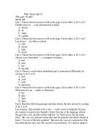
3.7.3 Inorder

Another variation of the algorithms defined in §3.7.1 and §3.7.2 is that of inorder
traversal where the value of the current node is yielded in between traversing
the left sub tree and the right sub tree. An example of inorder traversal is shown
in Figure 3.5.

23
14 31
7
17
9
23
14 31
7
9
23
14 31
7
9
23
14 31
7
9
23
14 31
7
9
23
14 31
7

(a) (b) (c)

(d) (e) (f)

17 17

17 17 17

Figure 3.5: Inorder visit binary search tree example

1) algorithm Inorder(root)

2) Pre: root is the root node of the BST

3) Post: the nodes in the BST have been visited in inorder
4) if root 6= ∅

5) Inorder(root.Left)
6) yield root.Value
7) Inorder(root.Right)
8) end if

9) end Inorder

</div>
(40)<div class='page_container' data-page=40>

were to traverse the tree in an inorder fashion then the values in the yielded
sequence would have the following properties n0≤ n1≤ nn.

3.7.4 Breadth First

Traversing a tree in breadth first order is to yield the values of all nodes of a
particular depth in the tree, e.g. given the depth d we would visit the values of
all nodes in a left to right fashion at d, then we would proceed to d + 1 and so
on until we had ran out of nodes to visit. An example of breadth first traversal
is shown in Figure 3.6.

Traditionally the way breadth first is implemented is using a list (vector,
resizeable array, etc) to store the values of the nodes visited in breadth first
order and then a queue to store those nodes that have yet to be visited.

14 31

9
23

14 31

(a) (b) (c)

(d) (e) (f)

17 17

17 17 17

</div>
(41)<div class='page_container' data-page=41>

CHAPTER 3. BINARY SEARCH TREE 30

1) algorithm BreadthFirst(root)

2) Pre: root is the root node of the BST

3) Post: the nodes in the BST have been visited in breadth first order
4) q ← queue

5) while root 6= ∅
6) yield root.Value
7) if root.Left 6= ∅

8) q.Enqueue(root.Left)

9) end if

10) if root.Right 6= ∅

11) q.Enqueue(root.Right)

12) end if

13) if !q.IsEmpty()

14) root ← q.Dequeue()

15) else

16) root ← ∅

17) end if
18) end while
19) end BreadthFirst

3.8 Summary

Binary search tree’s present a compelling solution when you want to have a
way to represent types that are ordered according to some custom rules that
are inherent for that particular type. With logarithmic insertion, lookup, and
deletion it is very effecient. Traversal remains linear, however as you have seen
there are many, many ways in which you can visit the nodes of a tree. Tree’s
are recursive data structures, so typically you will find that many algorithms
that operate on a tree are recursive.

</div>
(42)<div class='page_container' data-page=42>

Heap

A heap can be thought of as a simple tree data structure, however a heap usually
employs one of two strategies:

1. min heap; or

2. max heap

Each strategy determines the properties of the tree and it’s values, e.g. if
you were to choose the strategy min heap then each parent node would have
a value that is ≤ than it’s children, thus the node at the root of the tree will
have the smallest value in the tree, the opposite is true if you were to use a max
heap. Generally as a rule you should always assume that a heap employs the
min heap strategy unless otherwise stated.

Unlike other tree data structures like the one defined in §3 a heap is generally
implemented as an array rather than a series of nodes who each have references
to other nodes, both however contain nodes that have at most two children.
Figure 4.1 shows how the tree (not a heap data structure) (12 7(3 2) 6(9 ))
would be represented as an array. The array in Figure 4.1 is a result of simply
adding values in a top-to-bottom, left-to-right fashion. Figure 4.2 shows arrows
to the direct left and right child of each value in the array.

This chapter is very much centred around the notion of representing a tree as
an array and because this property is key to understanding this chapter Figure
4.3 shows a step by step process to represent a tree data structure as an array.
In Figure 4.3 you can assume that the default capacity of our array is eight.

Using just an array is often not sufficient as we have to be upfront about
the size of the array to use for the heap, often the run time behaviour of a
program can be unpredictable when it comes to the size of it’s internal data
structures thus we need to choose a more dynamic data structure that contains
the following properties:

1. we can specify an initial size of the array for scenarios when we know the
upper storage limit required; and

2. the data structure encapsulates resizing algorithms to grow the array as
required at run time

</div>
(43)<div class='page_container' data-page=43>

CHAPTER 4. HEAP 32

Figure 4.1: Array representation of a simple tree data structure

Figure 4.2: Direct children of the nodes in an array representation of a tree data
structure

1. Vector

2. ArrayList

3. List

In Figure 4.1 what might not be clear is how we would handle a null
ref-erence type. How we handle null values may change from project to project,
for example in one scenario we may be very strict and say you can’t add a
null object to the Heap. Other cases may dictate that a null object is given
the smallest value when comparing, similarly we may say that they might have
the maximum value when comparing. You will have to resolve this ambiguity
yourself having studied your requirements. Certainly for now it is much clearer
to think of none null objects being added to the heap.

Because we are using an array we need some way to calculate the index of
a parent node, and the children of a node, the required expressions for this are
defined as follows:

1. (index − 1)/2 (parent index)

2. 2 ∗ index + 1 (left child)

3. 2 ∗ index + 2 (right child)

In Figure 4.4 a) represents the calculation of the right child of 12 (2 ∗ 0 + 2);
and b) calculates the index of the parent of 3 ((3 − 1)/2).

4.1 Insertion

</div>
(44)<div class='page_container' data-page=44></div>
(45)<div class='page_container' data-page=45>

CHAPTER 4. HEAP 34

Figure 4.4: Calculating node properties

min heap ordering requires us to swap the values of a parent and it’s child if
the value of the child is < the value of it’s parent. We must do this for each sub
tree the value we just inserted is a constituent of.

The run time efficiency for heap insertion is O(log n). The run time is a
by product of verifying heap order as the first part of the algorithm (the actual
insertion into the array) is O(1).

</div>
(46)<div class='page_container' data-page=46></div>
(47)<div class='page_container' data-page=47>

CHAPTER 4. HEAP 36

1) algorithm Add(value)

2) Pre: value is the value to add to the heap
3) Count is the number of items in the heap
4) Post: the value has been added to the heap

5) heap[Count] ← value

6) Count ← Count +1
7) MinHeapify()
8) end Add

1) algorithm MinHeapify()

2) Pre: Count is the number of items in the heap
3) heap is the array used to store the heap items

4) Post: the heap has preserved min heap ordering
5) i ← Count −1

6) while i > 0 and heap[i] < heap[(i − 1)/2]
7) Swap(heap[i], heap[(i − 1)/2]

8) i ← (i − 1)/2

9) end while
10) end MinHeapify

The design of the MaxHeapify algorithm is very similar to that of the

Min-Heapify algorithm, the only difference is that the < operator in the second

condition of entering the while loop is changed to >.

4.2 Deletion

Just like when adding an item to the heap, when deleting an item from the heap
we must ensure that heap ordering is preserved. The algorithm for deletion has
three steps:

1. find the index of the value to delete

2. put the last value in the heap at the index location of the item to delete

</div>
(48)<div class='page_container' data-page=48>

1) algorithm Remove(value)

2) Pre: value is the value to remove from the heap

3) lef t, and right are updated alias’ for 2 ∗ index + 1, and 2 ∗ index + 2 respectively

4) Count is the number of items in the heap
5) heap is the array used to store the heap items

6) Post: value is located in the heap and removed, true; otherwise false
7) // step 1

8) index ← FindIndex(heap, value)

9) if index < 0
10) return false
11) end if

12) Count ← Count −1
13) // step 2

14) heap[index] ← heap[Count]

15) // step 3

16) while lef t < Count and heap[index] > heap[lef t] or heap[index] > heap[right]
17) // promote smallest key from sub tree

18) if heap[lef t] < heap[right]
19) Swap(heap, lef t, index)

20) index ← lef t

21) else

22) Swap(heap, right, index)

23) index ← right

24) end if
25) end while
26) return true
27) end Remove

Figure 4.6 shows the Remove algorithm visually, removing 1 from a heap
containing the values 1, 3, 9, 12, and 13. In Figure 4.6 you can assume that we
have specified that the backing array of the heap should have an initial capacity
of eight.

4.3 Searching

A simple searching algorithm for a heap is merely a case of traversing the items

in the heap array sequentially, thus this operation has a run time complexity of

O(n). The search can be thought of as one that uses a breadth first traversal

</div>
(49)<div class='page_container' data-page=49>

CHAPTER 4. HEAP 38

</div>
(50)<div class='page_container' data-page=50>

1) algorithm Contains(value)

2) Pre: value is the value to search the heap for
3) Count is the number of items in the heap
4) heap is the array used to store the heap items

5) Post: value is located in the heap, in which case true; otherwise false
6) i ← 0

7) while i < Count and heap[i] 6= value

8) i ← i + 1

9) end while
10) if i < Count
11) return true
12) else

13) return false
14) end if

15) end Contains

The problem with the previous algorithm is that we don’t take advantage

of the properties in which all values of a heap hold, that is the property of the
heap strategy being used. For instance if we had a heap that didn’t contain the
value 4 we would have to exhaust the whole backing heap array before we could
determine that it wasn’t present in the heap. Factoring in what we know about
the heap we can optimise the search algorithm by including logic which makes
use of the properties presented by a certain heap strategy.

Optimising to deterministically state that a value is in the heap is not that
straightforward, however the problem is a very interesting one. As an example
consider a min-heap that doesn’t contain the value 5. We can only rule that the
value is not in the heap if 5 > the parent of the current node being inspected
and < the current node being inspected ∀ nodes at the current level we are
traversing. If this is the case then 5 cannot be in the heap and so we can
provide an answer without traversing the rest of the heap. If this property is
not satisfied for any level of nodes that we are inspecting then the algorithm
will indeed fall back to inspecting all the nodes in the heap. The optimisation
that we present can be very common and so we feel that the extra logic within
the loop is justified to prevent the expensive worse case run time.

</div>
(51)<div class='page_container' data-page=51>

CHAPTER 4. HEAP 40

1) algorithm Contains(value)

2) Pre: value is the value to search the heap for
3) Count is the number of items in the heap
4) heap is the array used to store the heap items

5) Post: value is located in the heap, in which case true; otherwise false
6) start ← 0

7) nodes ← 1

8) while start < Count

9) start ← nodes − 1

10) end ← nodes + start

11) count ← 0

12) while start < Count and start < end
13) if value = heap[start]

14) return true

15) else if value > Parent(heap[start]) and value < heap[start]

16) count ← count + 1

17) end if

18) start ← start + 1

19) end while
20) if count = nodes
21) return false
22) end if

23) nodes ← nodes ∗ 2

24) end while
25) return false
26) end Contains

The new Contains algorithm determines if the value is not in the heap by
checking whether count = nodes. In such an event where this is true then we
can confirm that ∀ nodes n at level i : value > Parent(n), value < n thus there
is no possible way that value is in the heap. As an example consider Figure 4.7.
If we are searching for the value 10 within the min-heap displayed it is obvious
that we don’t need to search the whole heap to determine 9 is not present. We
can verify this after traversing the nodes in the second level of the heap as the
previous expression defined holds true.

4.4 Traversal

</div>
(52)<div class='page_container' data-page=52>

Figure 4.7: Determining 10 is not in the heap after inspecting the nodes of Level
2

4.5 Summary

Heaps are most commonly used to implement priority queues (see §6.2 for an
example implementation) and to facilitate heap sort. As discussed in both the
insertion §4.1, and deletion §4.2 sections a heap maintains heap order according
to the selected ordering strategy. These strategies are referred to as min-heap,
and max-heap. The former strategy enforces that the value of a parent node is
less than that of each of its children, the latter enforces that the value of the
parent is greater than that of each of its children.

</div>
(53)<div class='page_container' data-page=53>

Chapter 5 Sets

A set contains a number of values, the values are in no particular order and the
values within the set are distinct from one another.

Generally set implementations tend to check that a value is not in the set
first, before adding it to the set and so the issue of repeated values within the
set is not an issue.

This section does not cover set theory in depth, rather it demonstrates briefly
the ways in which the values of sets can be defined, and common operations that
may be performed upon them.

The following A = {4, 7, 9, 12, 0} defines a set A whose values are listed
within the curly braces.

Given the set A defined previously we can say that 4 is a member of A
denoted by 4 ∈ A, and that 99 is not a member of A denoted by 99 /∈ A.

Often defining a set by manually stating its members is tiresome, and more
importantly the set may contain a large amount of values. A more concise way
of defining a set and its members is by providing a series of properties that the
values of the set must satisfy. In the following A = {x|x > 0, x % 2 = 0} the
set A contains only positive integers that are even, x is an alias to the current
value we are inspecting and to the right hand side of | are the properties that x
must satisfy to be in the set A that is it must be > 0, and the remainder of the
arithmetic expression x/2 must be 0. You will be able to note from the previous
definition of the set A that the set can contain an infinite number of values, and
that the values of the set A will be all even integers that are a member of the
natural numbers set N, where N = {1, 2, 3, ...}.

Finally in this brief introduction to sets we will cover set intersection and
union, both of which are very common operations (amongst many others)
per-formed on sets. The union set can be defined as follows A ∪ B = {x | x ∈

A or x ∈ B}, and intersection A ∩ B = {x | x ∈ A and x ∈ B}. Figure 5.1

demonstrates set intersection and union graphically.

Given the following set definitions A = {1, 2, 3}, and B = {6, 2, 9} the union
of the two sets is A ∪ B = {1, 2, 3, 6, 9}, and the intersection of the two sets is

A ∩ B = {2}.

Both set union and intersection are sometimes provided within the
frame-work associated with mainstream languages, this is the case in .NET 3.51

1 />

</div>
(54)<div class='page_container' data-page=54>

Figure 5.1: a) A ∩ B; b) A ∪ B

where such algorithms exist as extension methods defined in the type

Sys-tem.Linq.Enumerable2, as a result DSA does not provide implementations of

these algorithms. Most of the algorithms defined in System.Linq.Enumerable
deal mainly with sequences rather than sets exclusively.

Set union can be implemented as a simple traversal of both sets adding each
item of the two sets to a new union set.

1) algorithm Union(set1, set2)
2) Pre: set1, and set2 6= ∅

3) union is a set

3) Post: A union of set1, and set2 has been created
4) foreach item in set1

5) union.Add(item)

6) end foreach

7) foreach item in set2

8) union.Add(item)

9) end foreach
10) return union
11) end Union

The run time of our Union algorithm is O(m + n) where m is the number
of items in the first set and n is the number of items in the second set.

Set intersection is also trivial to implement. The only major thing worth
pointing out about our algorithm is that we traverse the set containing the
fewest items. We can do this because if we have exhausted all the items in the
smaller of the two sets then there are no more items that are members of both
sets, thus we have no more items to add to the intersection set.

</div>
(55)<div class='page_container' data-page=55>

CHAPTER 5. SETS 44

1) algorithm Intersection(set1, set2)
2) Pre: set1, and set2 6= ∅

3) intersection, and smallerSet are sets

3) Post: An intersection of set1, and set2 has been created
4) if set1.Count < set2.Count

5) smallerSet ← set1

6) else

7) smallerSet ← set2

8) end if

9) foreach item in smallerSet

10) if set1.Contains(item) and set2.Contains(item)
11) intersection.Add(item)

12) end if
13) end foreach
14) return intersection
15) end Intersection

The run time of our Intersection algorithm is O(n) where n is the number
of items in the smaller of the two sets.

5.1 Unordered

Sets in the general sense do not enforce the explicit ordering of their members,
for example the members of B = {6, 2, 9} conform to no ordering scheme because
it is not required.

Most libraries provide implementations of unordered sets and so DSA does
not, we simply mention it here to disambiguate between an unordered set and
ordered set.

We will only look at insertion for an unordered set and cover briefly why a
hash table is an efficient data structure to use for its implementation.

5.1.1 Insertion

Unordered sets can be efficiently implemented using a hash table as its backing
data structure. As mentioned previously we only add an item to a set if that
item is not already in the set, thus the backing data structure we use must have
a quick look up and insertion run time complexity.

A hash map generally provides the following:

1. O(1) for insertion

2. approaching O(1) for look up

</div>
(56)<div class='page_container' data-page=56>

5.2 Ordered

An ordered set is similar to an unordered set in the sense that its members are
distinct, however an ordered set enforces some predefined comparison on each

of its members to result in a set whose members are ordered appropriately.

In DSA 0.5 and earlier we used a binary search tree (defined in §3) as the
internal backing data structure for our ordered set, from versions 0.6 onwards
we replaced the binary search tree with an AVL tree primarily because AVL is
balanced.

The ordered set has it’s order realised by performing an inorder traversal
upon its backing tree data structure which yields the correct ordered sequence
of set members.

Because an ordered set in DSA is simply a wrapper for an AVL tree that
additionally enforces the tree contains unique items you should read §7.1 to
learn more about the run time complexities associated with its operations.

5.3 Summary

Set’s provide a way of having a collection of unique objects, either ordered or
unordered.

When implementing a set (either ordered, or unordered) it is key to select
the correct backing data structure. As we discussed in §5.1.1 because we check
first if the item is already contained within the set before adding it we need
this check to be as quick as possible. For unordered sets we can rely on the use
of a hash table and use the key of an item to determine whether or not it is
already contained within the set. Using a hash table this check results in a near
constant run time complexity. Ordered sets cost a little more for this check,
however the logarithmic growth that we incur by using a binary search tree as
its backing data structure is acceptable.

Another key property of sets implemented using the approach we describe is
that both have favourably fast look-up times. Just like the check before
inser-tion, for a hash table this run time complexity should be near constant. Ordered
sets as described in 3 perform a binary chop at each stage when searching for
the existence of an item yielding a logarithmic run time.

</div>
(57)<div class='page_container' data-page=57>

Chapter 6 Queues

Queues are an essential data structure that have found themselves used in vast
amounts of software from user mode to kernel mode applications that are core
to the system. Fundamentally they honour a first in first out (FIFO) strategy,
that is the item first put into the queue will be the first served, the second item
added to the queue will be the second to be served and so on.

All queues only allow you to access the item at the front of the queue, when
you add an item to the queue that item is placed at the back of the queue.

Historically queues always have the following three core methods:

Enqueue: places an item at the back of the queue;

Dequeue: retrieves the item at the front of the queue, and removes it from the
queue;

Front: 1 retrieves the item at the front of the queue without removing it from

the queue

As an example to demonstrate the behaviour of a queue we will walk through
a scenario whereby we invoke each of the previously mentioned methods
observ-ing the mutations upon the queue data structure, the followobserv-ing list describes
the operations performed upon the queue in Figure 6.1:

1. Enqueue(10)

2. Enqueue(12)

3. Enqueue(9)

4. Enqueue(8)

5. Enqueue(3)

6. Dequeue()

7. Front()

8. Enqueue(33)

1This operation is sometimes referred to as Peek

</div>
(58)<div class='page_container' data-page=58>

9. Front()

10. Dequeue()

6.1 Standard Queue

A queue is implicitly like that described prior to this section, in DSA we don’t

provide a standard queue because queues are so popular and such a core data
structure you will find that pretty much every mainstream library provides a
queue data structure that you can use with your language of choice. In this
section we will discuss how you can, if required implement an efficient queue
data structure.

The main property of a queue is that we have access to the item at the
front of the queue, the queue data structure can be efficiently implemented
using a singly linked list (defined in §2.1). A singly linked list provides O(1)
insertion, and deletion run time complexities - the reason we have an O(1) run
time complexity for deletion is because we only ever in a queue remove the item
at the front (Dequeue) and since we always have a pointer to the item at the
head of a singly linked list removal is simply a case of returning the value of
the old head node, and then modifying the head pointer to be the next node of
the old head node. The run time complexity for searching a queue remains the
same as that of a singly linked list, O(n).

6.2 Priority Queue

Unlike a standard queue where items are ordered in terms of who arrived first,
a priority queue determines the order of its items by using a form of custom
comparer to see which item has the highest priority. Other than the items in a
priority queue being ordered by priority it remains the same as a normal queue,
you can only access the item at the front of the queue.

A sensible implementation of a priority queue is to use a heap data structure
(defined in §4). Using a heap we can look at the first item in the queue by simply
returning the item at index 0 within the heap array. A heap provides us with
the ability to construct a priority queue where by the items with the highest
priority are either those with the smallest value, or those with the largest.

6.3 Summary

With normal queues we have seen that those who arrive first are dealt with
first, that is they are dealt with in a first-in-first-out (FIFO) order. Queues can
be ever so useful, e.g. the Windows CPU scheduler uses a different queue for
each priority of process to determine who should be the next process to utilise
the CPU for a specified time quantum. Normal queues have constant insertion,
and deletion run times. Searching a queue is fairly unnatural in the sense that
typically you are only interested in the item at the front of the queue, despite
that searching is usually exposed on queues which has a linear run time.

</div>
(59)<div class='page_container' data-page=59>

CHAPTER 6. QUEUES 48

</div>
(60)<div class='page_container' data-page=60>

priority queue as mentioned in this chapter uses a heap data structure as its
backing store, thus the run times for insertion, deletion, and searching is the
same as those for a heap (defined in §4).

</div>
(61)<div class='page_container' data-page=61>

Chapter 7 Balanced Trees

7.1 AVL Tree

</div>
(62)<div class='page_container' data-page=62>

Algorithms

</div>
(63)<div class='page_container' data-page=63>

Chapter 8 Sorting

All the sorting algorithms in this chapter use data structures of a specific type
to demonstrate sorting, e.g. a 32 bit integer is often used as its associated
operations (e.g. <, >, etc) are clear in their behaviour.

The algorithms discussed can easily be translated into generic sorting
algo-rithms within your respective language of choice.

8.1 Bubble Sort

One of the most simple forms of sorting is that of comparing each item with
every other item in some list, however as the description may imply this form
of sorting is not particularly effecient O(n2). In it’s most simple form bubble

sort can be implemented as two loops.
1) algorithm BubbleSort(list)
2) Pre: list 6= ∅

3) Post: list has been sorted into values of ascending order
4) for i ← 0 to list.Count − 1

5) for j ← 0 to list.Count − 1
6) if list[i] < list[j]
7) Swap(list[i], list[j])

8) end if

9) end for
10) end for
11) return list
12) end BubbleSort

8.2 Merge Sort

Merge sort is an algorithm that has a fairly efficient space time complexity

-O(n log n) and is fairly trivial to implement. The algorithm is based on splitting

a list, into two similar sized lists (lef t, and right) and sorting each list and then
merging the sorted lists back together.

Note: the function MergeOrdered simply takes two ordered lists and makes
them one.

</div>
(64)<div class='page_container' data-page=64>

54
2
74
75
4

0 1 2 3 4

54
2
74
75
4

0 1 2 3 4

2
75
74
4

0 1 2 3 4

54
75
2
74
4

0 1 2 3 4

75
54
2
74
4

0 1 2 3 4

75
54
2
74
4

0 1 2 3 4

75
54
2
74
4

0 1 2 3 4

75
54
74
2
4

0 1 2 3 4

75
74
54
2
4

0 1 2 3 4

75
74
54
2
4

0 1 2 3 4

75
74
54
4
2

0 1 2 3 4

75
74
54
4
2

0 1 2 3 4

75
74
54
4
2

0 1 2 3 4

75
74
54

4
2

0 1 2 3 4

75
74
54
4
2

0 1 2 3 4

Figure 8.1: Bubble Sort Iterations

1) algorithm Mergesort(list)
2) Pre: list 6= ∅

3) Post: list has been sorted into values of ascending order
4) if list.Count = 1 // already sorted

5) return list
6) end if

7) m ← list.Count / 2

8) lef t ← list(m)

9) right ← list(list.Count − m)

10) for i ← 0 to lef t.Count−1
11) lef t[i] ← list[i]

12) end for

13) for i ← 0 to right.Count−1
14) right[i] ← list[i]

15) end for

16) lef t ← Mergesort(lef t)

17) right ← Mergesort(right)

</div>
(65)<div class='page_container' data-page=65>

CHAPTER 8. SORTING 54
54
2
74
75
4
75
4
54
2
74
4
75
74
54
2

2
5
4
Divide
54
2
75
4
74
54
2
75
74
54
4
2
Impera(Merge)

Figure 8.2: Merge Sort Divide et Impera Approach

8.3 Quick Sort

Quick sort is one of the most popular sorting algorithms based on divide et
impera strategy, resulting in an O(n log n) complexity. The algorithm starts by
picking an item, called pivot, and moving all smaller items before it, while all
greater elements after it. This is the main quick sort operation, called partition,
recursively repeated on lesser and greater sub lists until their size is one or zero
- in which case the list is implicitly sorted.

</div>
(66)<div class='page_container' data-page=66>

2
74
75
4
Pivot
54
2
74
75
4
Pivot
75
2
74
54
4
Pivot
75
54
74
2
4
Pivot
75
74
54
2
4
Pivot
2

4
Pivot
4
2
Pivot
75
74
Pivot
75
74
75
74
54
4
2
Pivot

Figure 8.3: Quick Sort Example (pivot median strategy)

1) algorithm QuickSort(list)
2) Pre: list 6= ∅

3) Post: list has been sorted into values of ascending order
4) if list.Count = 1 // already sorted

5) return list
6) end if

7) pivot ←MedianValue(list)

8) for i ← 0 to list.Count−1
9) if list[i] = pivot
10) equal.Insert(list[i])

11) end if

12) if list[i] < pivot
13) less.Insert(list[i])

14) end if

15) if list[i] > pivot

16) greater.Insert(list[i])

17) end if
18) end for

</div>
(67)<div class='page_container' data-page=67>

CHAPTER 8. SORTING 56

8.4 Insertion Sort

Insertion sort is a somewhat interesting algorithm with an expensive runtime of

O(n2). It can be best thought of as a sorting scheme similar to that of sorting

a hand of playing cards, i.e. you take one card and then look at the rest with
the intent of building up an ordered set of cards in your hand.

2
74
75

4 4 75 74 2 54 4 75 74 2 54

74
54
2
75
74
4
2
75
54
75
74
4
2
54
75
74
54
4
2
4

Figure 8.4: Insertion Sort Iterations

1) algorithm Insertionsort(list)

2) Pre: list 6= ∅

3) Post: list has been sorted into values of ascending order
4) unsorted ← 1

5) while unsorted < list.Count
6) hold ← list[unsorted]

7) i ← unsorted − 1

8) while i ≥ 0 and hold < list[i]
9) list[i + 1] ← list[i]

10) i ← i − 1

11) end while
12) list[i + 1] ← hold

13) unsorted ← unsorted + 1

</div>
(68)<div class='page_container' data-page=68>

8.5 Shell Sort

Put simply shell sort can be thought of as a more efficient variation of insertion
sort as described in §8.4, it achieves this mainly by comparing items of varying
distances apart resulting in a run time complexity of O(n log2 n).

Shell sort is fairly straight forward but may seem somewhat confusing at
first as it differs from other sorting algorithms in the way it selects items to
compare. Figure 8.5 shows shell sort being ran on an array of integers, the red
coloured square is the current value we are holding.

1) algorithm ShellSort(list)
2) Pre: list 6= ∅

3) Post: list has been sorted into values of ascending order
4) increment ← list.Count / 2

5) while increment 6= 0

6) current ← increment

7) while current < list.Count

8) hold ← list[current]

9) i ← current − increment

10) while i ≥ 0 and hold < list[i]

11) list[i + increment] ← list[i]

12) i− = increment

13) end while

14) list[i + increment] ← hold

15) current ← current + 1

16) end while

17) increment / = 2

18) end while
19) return list
20) end ShellSort

8.6 Radix Sort

</div>
(69)<div class='page_container' data-page=69>

CHAPTER 8. SORTING 58

</div>
(70)<div class='page_container' data-page=70>

1. Ones

2. Tens

3. Hundreds

For further clarification what if we wanted to determine how many thousands
the number 102 has? Clearly there are none, but often looking at a number as
final like we often do it is not so obvious so when asked the question how many
thousands does 102 have you should simply pad the number with a zero in that
location, e.g. 0102 here it is more obvious that the key value at the thousands
location is zero.

The last thing to identify before we actually show you a simple
implemen-tation of radix sort that works on only positive integers, and requires you to
specify the maximum key size in the list is that we need a way to isolate a
specific key at any one time. The solution is actually very simple, but its not
often you want to isolate a key in a number so we will spell it out clearly
here. A key can be accessed from any integer with the following expression:

key ← (number / keyT oAccess) % 10. As a simple example lets say that we

want to access the tens key of the number 1290, the tens column is key 10 and
so after substitution yields key ← (1290 / 10) % 10 = 9. The next key to
look at for a number can be attained by multiplying the last key by ten working
left to right in a sequential manner. The value of key is used in the following
algorithm to work out the index of an array of queues to enqueue the item into.
1) algorithm Radix(list, maxKeySize)

2) Pre: list 6= ∅

3) maxKeySize ≥ 0 and represents the largest key size in the list

4) Post: list has been sorted
5) queues ← Queue[10]

6) indexOf Key ← 1

7) fori ← 0 to maxKeySize − 1
8) foreach item in list

9) queues[GetQueueIndex(item, indexOf Key)].Enqueue(item)

10) end foreach

11) list ← CollapseQueues(queues)

12) ClearQueues(queues)

13) indexOf Key ← indexOf Key ∗ 10

14) end for
15) return list
16) end Radix

Figure 8.6 shows the members of queues from the algorithm described above
operating on the list whose members are 90, 12, 8, 791, 123, and 61, the key we
are interested in for each number is highlighted. Omitted queues in Figure 8.6
mean that they contain no items.

8.7 Summary

</div>
(71)<div class='page_container' data-page=71>

CHAPTER 8. SORTING 60

Figure 8.6: Radix sort base 10 algorithm

bubble sort defined in §8.1).

Selecting the correct sorting algorithm is usually denoted purely by efficiency,
e.g. you would always choose merge sort over shell sort and so on. There are
also other factors to look at though and these are based on the actual
imple-mentation. Some algorithms are very nicely expressed in a recursive fashion,
however these algorithms ought to be pretty efficient, e.g. implementing a linear,
quadratic, or slower algorithm using recursion would be a very bad idea.

</div>
(72)<div class='page_container' data-page=72>

Numeric

Unless stated otherwise the alias n denotes a standard 32 bit integer.

9.1 Primality Test

A simple algorithm that determines whether or not a given integer is a prime
number, e.g. 2, 5, 7, and 13 are all prime numbers, however 6 is not as it can
be the result of the product of two numbers that are < 6.

In an attempt to slow down the inner loop the √n is used as the upper

bound.

1) algorithm IsPrime(n)

2) Post: n is determined to be a prime or not
3) for i ← 2 to n do

4) for j ← 1 to sqrt(n) do
5) if i ∗ j = n

6) return false

7) end if

8) end for
9) end for
10) end IsPrime

9.2 Base conversions

DSA contains a number of algorithms that convert a base 10 number to its
equivalent binary, octal or hexadecimal form. For example 7810 has a binary

representation of 10011102.

Table 9.1 shows the algorithm trace when the number to convert to binary
is 74210.

</div>
(73)<div class='page_container' data-page=73>

CHAPTER 9. NUMERIC 62

1) algorithm ToBinary(n)
2) Pre: n ≥ 0

3) Post: n has been converted into its base 2 representation
4) while n > 0

5) list.Add(n % 2)

6) n ← n/2

7) end while

8) return Reverse(list)
9) end ToBinary

n list

742 { 0 }

371 { 0, 1 }

185 { 0, 1, 1 }

92 { 0, 1, 1, 0 }

46 { 0, 1, 1, 0, 1 }

23 { 0, 1, 1, 0, 1, 1 }

11 { 0, 1, 1, 0, 1, 1, 1 }

5 { 0, 1, 1, 0, 1, 1, 1, 1 }

2 { 0, 1, 1, 0, 1, 1, 1, 1, 0 }

1 { 0, 1, 1, 0, 1, 1, 1, 1, 0, 1 }

Table 9.1: Algorithm trace of ToBinary

9.3 Attaining the greatest common

denomina-tor of two numbers

A fairly routine problem in mathematics is that of finding the greatest common
denominator of two integers, what we are essentially after is the greatest number
which is a multiple of both, e.g. the greatest common denominator of 9, and
15 is 3. One of the most elegant solutions to this problem is based on Euclid’s
algorithm that has a run time complexity of O(n2).

1) algorithm GreatestCommonDenominator(m, n)
2) Pre: m and n are integers

3) Post: the greatest common denominator of the two integers is calculated
4) if n = 0

5) return m
6) end if

</div>
(74)<div class='page_container' data-page=74>

9.4 Computing the maximum value for a

num-ber of a specific base consisting of N digits

This algorithm computes the maximum value of a number for a given number
of digits, e.g. using the base 10 system the maximum number we can have
made up of 4 digits is the number 999910. Similarly the maximum number that

consists of 4 digits for a base 2 number is 11112 which is 1510.

The expression by which we can compute this maximum value for N digits
is: BN − 1. In the previous expression B is the number base, and N is the

number of digits. As an example if we wanted to determine the maximum value
for a hexadecimal number (base 16) consisting of 6 digits the expression would
be as follows: 166− 1. The maximum value of the previous example would be

represented as F F F F F F16 which yields 1677721510.

In the following algorithm numberBase should be considered restricted to
the values of 2, 8, 9, and 16. For this reason in our actual implementation

numberBase has an enumeration type. The Base enumeration type is defined

as:

Base = {Binary ← 2, Octal ← 8, Decimal ← 10, Hexadecimal ← 16}

The reason we provide the definition of Base is to give you an idea how this
algorithm can be modelled in a more readable manner rather than using various
checks to determine the correct base to use. For our implementation we cast the
value of numberBase to an integer, as such we extract the value associated with
the relevant option in the Base enumeration. As an example if we were to cast
the option Octal to an integer we would get the value 8. In the algorithm listed
below the cast is implicit so we just use the actual argument numberBase.
1) algorithm MaxValue(numberBase, n)

2) Pre: numberBase is the number system to use, n is the number of digits
3) Post: the maximum value for numberBase consisting of n digits is computed
4) return Power(numberBase, n) −1

5) end MaxValue

9.5 Factorial of a number

Attaining the factorial of a number is a primitive mathematical operation. Many
implementations of the factorial algorithm are recursive as the problem is
re-cursive in nature, however here we present an iterative solution. The iterative
solution is presented because it too is trivial to implement and doesn’t suffer
from the use of recursion (for more on recursion see §C).

</div>
(75)<div class='page_container' data-page=75>

CHAPTER 9. NUMERIC 64

1) algorithm Factorial(n)

2) Pre: n ≥ 0, n is the number to compute the factorial of
3) Post: the factorial of n is computed

4) if n < 2
5) return 1
6) end if
7) f actorial ← 1

8) for i ← 2 to n

9) f actorial ← f actorial ∗ i

10) end for

</div>
(76)<div class='page_container' data-page=76>

Searching

10.1 Sequential Search

A simple algorithm that search for a specific item inside a list. It operates
looping on each element O(n) until a match occurs or the end is reached.
1) algorithm SequentialSearch(list, item)

2) Pre: list 6= ∅

3) Post: return index of item if found, otherwise −1
4) index ← 0

5) while index < list.Count and list[index] 6= item

6) index ← index + 1

7) end while

8) if index < list.Count and list[index] = item
9) return index

10) end if
11) return −1

12) end SequentialSearch

10.2 Probability Search

Probability search is a statistical sequential searching algorithm. In addition to
searching for an item, it takes into account its frequency by swapping it with
it’s predecessor in the list. The algorithm complexity still remains at O(n) but
in a non-uniform items search the more frequent items are in the first positions,
reducing list scanning time.

Figure 10.1 shows the resulting state of a list after searching for two items,
notice how the searched items have had their search probability increased after
each search operation respectively.

</div>
(77)<div class='page_container' data-page=77>

CHAPTER 10. SEARCHING 66

Figure 10.1: a) Search(12), b) Search(101)

1) algorithm ProbabilitySearch(list, item)
2) Pre: list 6= ∅

3) Post: a boolean indicating where the item is found or not;
in the former case swap founded item with its predecessor

4) index ← 0

5) while index < list.Count and list[index] 6= item

6) index ← index + 1

7) end while

8) if index ≥ list.Count or list[index] 6= item
9) return false

10) end if
11) if index > 0

12) Swap(list[index], list[index − 1])

13) end if
14) return true

</div>
(78)<div class='page_container' data-page=78>

Sets

</div>
(79)<div class='page_container' data-page=79>

Chapter 12 Strings

Strings have their own chapter in this text purely because string operations
and transformations are incredibly frequent within programs. The algorithms
presented are based on problems the authors have come across previously, or
were formulated to satisfy curiosity.

12.1 Reversing the order of words in a sentence

Defining algorithms for primitive string operations is simple, e.g. extracting a
sub-string of a string, however some algorithms that require more inventiveness
can be a little more tricky.

The algorithm presented here does not simply reverse the characters in a
string, rather it reverses the order of words within a string. This algorithm
works on the principal that words are all delimited by white space, and using a
few markers to define where words start and end we can easily reverse them.

</div>
(80)<div class='page_container' data-page=80>

1) algorithm ReverseWords(value)

2) Pre: value 6= ∅, sb is a string buffer

3) Post: the words in value have been reversed
4) last ← value.Length − 1

5) start ← last

6) while last ≥ 0

7) // skip whitespace

8) while start ≥ 0 and value[start] = whitespace

9) start ← start − 1

10) end while

11) last ← start

12) // march down to the index before the beginning of the word
13) while start ≥ 0 and start 6= whitespace

14) start ← start − 1

15) end while

16) // append chars from start + 1 to length + 1 to string buffer sb
17) for i ← start + 1 to last

18) sb.Append(value[i])

19) end for

20) // if this isn’t the last word in the string add some whitespace after the word in the buffer
21) if start > 0

22) sb.Append(‘ ’)

23) end if

24) last ← start − 1

25) start ← last

26) end while

27) // check if we have added one too many whitespace to sb

28) if sb[sb.Length −1] = whitespace

29) // cut the whitespace
30) sb.Length ← sb.Length −1

31) end if
32) return sb
33) end ReverseWords

12.2 Detecting a palindrome

Although not a frequent algorithm that will be applied in real-life scenarios
detecting a palindrome is a fun, and as it turns out pretty trivial algorithm to
design.

The algorithm that we present has a O(n) run time complexity. Our 
algo-rithm uses two pointers at opposite ends of string we are checking is a palindrome
or not. These pointers march in towards each other always checking that each
character they point to is the same with respect to value. Figure 12.1 shows the

IsPalindrome algorithm in operation on the string “Was it Eliot’s toilet I saw?”

</div>
(81)<div class='page_container' data-page=81>

CHAPTER 12. STRINGS 70

Figure 12.1: lef t and right pointers marching in towards one another

1) algorithm IsPalindrome(value)
2) Pre: value 6= ∅

3) Post: value is determined to be a palindrome or not

4) word ← value.Strip().ToUpperCase()

5) lef t ← 0

6) right ← word.Length −1

7) while word[lef t] = word[right] and lef t < right
8) lef t ← lef t + 1

9) right ← right − 1

10) end while

11) return word[lef t] = word[right]
12) end IsPalindrome

In the IsPalindrome algorithm we call a method by the name of Strip. This
algorithm discards punctuation in the string, including white space. As a result

word contains a heavily compacted representation of the original string, each

character of which is in its uppercase representation.

Palindromes discard white space, punctuation, and case making these changes
allows us to design a simple algorithm while making our algorithm fairly robust
with respect to the palindromes it will detect.

12.3 Counting the number of words in a string

Counting the number of words in a string can seem pretty trivial at first, however

there are a few cases that we need to be aware of:

1. tracking when we are in a string

2. updating the word count at the correct place

3. skipping white space that delimits the words

As an example consider the string “Ben ate hay” Clearly this string contains
three words, each of which distinguished via white space. All of the previously
listed points can be managed by using three variables:

1. index

2. wordCount

</div>
(82)<div class='page_container' data-page=82>

Figure 12.2: String with three words

Figure 12.3: String with varying number of white space delimiting the words

Of the previously listed index keeps track of the current index we are at in
the string, wordCount is an integer that keeps track of the number of words we
have encountered, and finally inW ord is a Boolean flag that denotes whether
or not at the present time we are within a word. If we are not currently hitting
white space we are in a word, the opposite is true if at the present index we are
hitting white space.

What denotes a word? In our algorithm each word is separated by one or
more occurrences of white space. We don’t take into account any particular
splitting symbols you may use, e.g. in .NET String.Split1 can take a char (or

array of characters) that determines a delimiter to use to split the characters
within the string into chunks of strings, resulting in an array of sub-strings.

In Figure 12.2 we present a string indexed as an array. Typically the pattern
is the same for most words, delimited by a single occurrence of white space.
Figure 12.3 shows the same string, with the same number of words but with
varying white space splitting them.

</div>
(83)<div class='page_container' data-page=83>

CHAPTER 12. STRINGS 72

1) algorithm WordCount(value)
2) Pre: value 6= ∅

3) Post: the number of words contained within value is determined
4) inW ord ← true

5) wordCount ← 0

6) index ← 0

7) // skip initial white space

8) while value[index] = whitespace and index < value.Length −1

9) index ← index + 1

10) end while

11) // was the string just whitespace?

12) if index = value.Length and value[index] = whitespace
13) return 0

14) end if

15) while index < value.Length
16) if value[index] = whitespace
17) // skip all whitespace

18) while value[index] = whitespace and index < value.Length −1

19) index ← index + 1

20) end while

21) inW ord ← f alse

22) wordCount ← wordCount + 1

23) else

24) inW ord ← true

25) end if

26) index ← index + 1

27) end while

28) // last word may have not been followed by whitespace
29) if inW ord

30) wordCount ← wordCount + 1

31) end if

32) return wordCount
33) end WordCount

12.4 Determining the number of repeated words

within a string

</div>
(84)<div class='page_container' data-page=84>

Figure 12.4: a) Undesired uniques set; b) desired uniques set

1) algorithm RepeatedWordCount(value)
2) Pre: value 6= ∅

3) Post: the number of repeated words in value is returned
4) words ← value.Split(’ ’)

5) uniques ← Set

6) foreach word in words
7) uniques.Add(word.Strip())

8) end foreach

9) return words.Length −uniques.Count
10) end RepeatedWordCount

You will notice in the RepeatedWordCount algorithm that we use the Strip
method we referred to earlier in §12.1. This simply removes any punctuation
from a word. The reason we perform this operation on each word is so that
we can build a more accurate unique string collection, e.g. “test”, and “test!”
are the same word minus the punctuation. Figure 12.4 shows the undesired and
desired sets for the unique set respectively.

12.5 Determining the first matching character

between two strings

</div>
(85)<div class='page_container' data-page=85>

CHAPTER 12. STRINGS 74

t
s
e
t

0 1 2 3 4

s
r
e
t
p

0 1 2 3 4 5 6

Word
Match

i
t
s
e
t

0 1 2 3 4

s
r
e
t
p

0 1 2 3 4 5 6

i
index
t
s
e
t

0 1 2 3 4

s
r
e
t
p

0 1 2 3 4 5 6

index
index

a) b) c)

Figure 12.5: a) First Step; b) Second Step c) Match Occurred

1) algorithm Any(word,match)
2) Pre: word, match 6= ∅

3) Post: index representing match location if occured, −1 otherwise
4) for i ← 0 to word.Length − 1

5) while word[i] = whitespace

6) i ← i + 1

7) end while

8) for index ← 0 to match.Length − 1
9) while match[index] = whitespace

10) index ← index + 1

11) end while

12) if match[index] = word[i]
13) return index

</div>
(86)<div class='page_container' data-page=86>

Algorithm Walkthrough

Learning how to design good algorithms can be assisted greatly by using a
structured approach to tracing its behaviour. In most cases tracing an algorithm
only requires a single table. In most cases tracing is not enough, you will also
want to use a diagram of the data structure your algorithm operates on. This
diagram will be used to visualise the problem more effectively. Seeing things
visually can help you understand the problem quicker, and better.

The trace table will store information about the variables used in your
algo-rithm. The values within this table are constantly updated when the algorithm
mutates them. Such an approach allows you to attain a history of the various
values each variable has held. You may also be able to infer patterns from the
values each variable has contained so that you can make your algorithm more
efficient.

We have found this approach both simple, and powerful. By combining a
visual representation of the problem as well as having a history of past values
generated by the algorithm it can make understanding, and solving problems
much easier.

In this chapter we will show you how to work through both iterative, and
recursive algorithms using the technique outlined.

A.1 Iterative algorithms

We will trace the IsPalindrome algorithm (defined in §12.2) as our example
iterative walkthrough. Before we even look at the variables the algorithm uses,
first we will look at the actual data structure the algorithm operates on. It
should be pretty obvious that we are operating on a string, but how is this
represented? A string is essentially a block of contiguous memory that consists
of some char data types, one after the other. Each character in the string can
be accessed via an index much like you would do when accessing items within
an array. The picture should be presenting itself - a string can be thought of as
an array of characters.

For our example we will use IsPalindrome to operate on the string “Never
odd or even” Now we know how the string data structure is represented, and
the value of the string we will operate on let’s go ahead and draw it as shown
in Figure A.1.

</div>
(87)<div class='page_container' data-page=87>

APPENDIX A. ALGORITHM WALKTHROUGH 76

Figure A.1: Visualising the data structure we are operating on

value word lef t right

Table A.1: A column for each variable we wish to track

The IsPalindrome algorithm uses the following list of variables in some form
throughout its execution:

1. value

2. word

3. lef t

4. right

Having identified the values of the variables we need to keep track of we
simply create a column for each in a table as shown in Table A.1.

Now, using the IsPalindrome algorithm execute each statement updating
the variable values in the table appropriately. Table A.2 shows the final table
values for each variable used in IsPalindrome respectively.

While this approach may look a little bloated in print, on paper it is much
more compact. Where we have the strings in the table you should annotate
these strings with array indexes to aid the algorithm walkthrough.

There is one other point that we should clarify at this time - whether to
include variables that change only a few times, or not at all in the trace table.
In Table A.2 we have included both the value, and word variables because it
was convenient to do so. You may find that you want to promote these values
to a larger diagram (like that in Figure A.1) and only use the trace table for
variables whose values change during the algorithm. We recommend that you
promote the core data structure being operated on to a larger diagram outside
of the table so that you can interrogate it more easily.

value word lef t right

“Never odd or even” “NEVERODDOREVEN” 0 13

1 12

2 11

3 10

4 9

5 8

6 7

7 6

</div>
(88)<div class='page_container' data-page=88>

We cannot stress enough how important such traces are when designing
your algorithm. You can use these trace tables to verify algorithm correctness.
At the cost of a simple table, and quick sketch of the data structure you are
operating on you can devise correct algorithms quicker. Visualising the problem
domain and keeping track of changing data makes problems a lot easier to solve.
Moreover you always have a point of reference which you can look back on.

A.2 Recursive Algorithms

For the most part working through recursive algorithms is as simple as walking
through an iterative algorithm. One of the things that we need to keep track
of though is which method call returns to who. Most recursive algorithms are
much simple to follow when you draw out the recursive calls rather than using
a table based approach. In this section we will use a recursive implementation
of an algorithm that computes a number from the Fiboncacci sequence.
1) algorithm Fibonacci(n)

2) Pre: n is the number in the fibonacci sequence to compute

3) Post: the fibonacci sequence number n has been computed
4) if n < 1

5) return 0
6) else if n < 2
7) return 1
8) end if

9) return Fibonacci(n − 1) + Fibonacci(n − 2)
10) end Fibonacci

Before we jump into showing you a diagrammtic representation of the
algo-rithm calls for the Fibonacci algoalgo-rithm we will briefly talk about the cases of
the algorithm. The algorithm has three cases in total:

1. n < 1

2. n < 2

3. n ≥ 2

The first two items in the preceeding list are the base cases of the algorithm.
Until we hit one of our base cases in our recursive method call tree we won’t
return anything. The third item from the list is our recursive case.

With each call to the recursive case we etch ever closer to one of our base
cases. Figure A.2 shows a diagrammtic representation of the recursive call chain.
In Figure A.2 the order in which the methods are called are labelled. Figure
A.3 shows the call chain annotated with the return values of each method call
as well as the order in which methods return to their callers. In Figure A.3 the

return values are represented as annotations to the red arrows.

</div>
(89)<div class='page_container' data-page=89>

APPENDIX A. ALGORITHM WALKTHROUGH 78

Figure A.2: Call chain for Fibonacci algorithm

</div>
(90)<div class='page_container' data-page=90>

the caller and continue execution of that method. Execution in the caller is
contiued at the next statement, or expression after the recursive call was made.
In the Fibonacci algorithms’ recursive case we make two recursive calls.
When the first recursive call (Fibonacci(n − 1)) returns to the caller we then
execute the the second recursive call (Fibonacci(n − 2)). After both recursive
calls have returned to their caller, the caller can then subesequently return to
its caller and so on.

Recursive algorithms are much easier to demonstrate diagrammatically as
Figure A.2 demonstrates. When you come across a recursive algorithm draw
method call diagrams to understand how the algorithm works at a high level.

A.3 Summary

Understanding algorithms can be hard at times, particularly from an
implemen-tation perspective. In order to understand an algorithm try and work through
it using trace tables. In cases where the algorithm is also recursive sketch the
recursive calls out so you can visualise the call/return chain.

</div>
(91)<div class='page_container' data-page=91>

Appendix B

Translation Walkthrough

The conversion from pseudo to an actual imperative language is usually very

straight forward, to clarify an example is provided. In this example we will
convert the algorithm in §9.1 to the C# language.

1) public static bool IsPrime(int number)
2) {

3) if (number < 2)
4) {

5) return false;
6) }

7) int innerLoopBound = (int)Math.Floor(Math.Sqrt(number));
8) for (int i = 1; i < number; i++)

9) {

10) for(int j = 1; j <= innerLoopBound; j++)
11) {

12) if (i ∗ j == number)

13) {

14) return false;

15) }

16) }

17) }

18) return true;
19) }

For the most part the conversion is a straight forward process, however you
may have to inject various calls to other utility algorithms to ascertain the
correct result.

A consideration to take note of is that many algorithms have fairly strict
preconditions, of which there may be several - in these scenarios you will need
to inject the correct code to handle such situations to preserve the correctness of
the algorithm. Most of the preconditions can be suitably handled by throwing
the correct exception.

</div>
(92)<div class='page_container' data-page=92>

B.1 Summary

As you can see from the example used in this chapter we have tried to make the
translation of our pseudo code algorithms to mainstream imperative languages
as simple as possible.

</div>
(93)<div class='page_container' data-page=93>

Appendix C

Recursive Vs. Iterative

Solutions

One of the most succinct properties of modern programming languages like
C++, C#, and Java (as well as many others) is that these languages allow
you to define methods that reference themselves, such methods are said to be
recursive. One of the biggest advantages recursive methods bring to the table is

that they usually result in more readable, and compact solutions to problems.

A recursive method then is one that is defined in terms of itself. Generally
a recursive algorithms has two main properties:

1. One or more base cases; and

2. A recursive case

For now we will briefly cover these two aspects of recursive algorithms. With
each recursive call we should be making progress to our base case otherwise we
are going to run into trouble. The trouble we speak of manifests itself typically
as a stack overflow, we will describe why later.

Now that we have briefly described what a recursive algorithm is and why
you might want to use such an approach for your algorithms we will now talk
about iterative solutions. An iterative solution uses no recursion whatsoever.
An iterative solution relies only on the use of loops (e.g. for, while, do-while,
etc). The down side to iterative algorithms is that they tend not to be as clear
as to their recursive counterparts with respect to their operation. The major
advantage of iterative solutions is speed. Most production software you will
find uses little or no recursive algorithms whatsoever. The latter property can
sometimes be a companies prerequisite to checking in code, e.g. upon checking
in a static analysis tool may verify that the code the developer is checking in
contains no recursive algorithms. Normally it is systems level code that has this
zero tolerance policy for recursive algorithms.

Using recursion should always be reserved for fast algorithms, you should
avoid it for the following algorithm run time deficiencies:

1. O(n2)

2. O(n3)

</div>
(94)<div class='page_container' data-page=94>

3. O(2n)

If you use recursion for algorithms with any of the above run time efficiency’s
you are inviting trouble. The growth rate of these algorithms is high and in
most cases such algorithms will lean very heavily on techniques like divide and
conquer. While constantly splitting problems into smaller problems is good
practice, in these cases you are going to be spawning a lot of method calls. All
this overhead (method calls don’t come that cheap) will soon pile up and either
cause your algorithm to run a lot slower than expected, or worse, you will run
out of stack space. When you exceed the allotted stack space for a thread the
process will be shutdown by the operating system. This is the case irrespective
of the platform you use, e.g. .NET, or native C++ etc. You can ask for a bigger
stack size, but you typically only want to do this if you have a very good reason
to do so.

C.1 Activation Records

An activation record is created every time you invoke a method. Put simply
an activation record is something that is put on the stack to support method
invocation. Activation records take a small amount of time to create, and are
pretty lightweight.

Normally an activation record for a method call is as follows (this is very
general):

• The actual parameters of the method are pushed onto the stack

• The return address is pushed onto the stack

• The top-of-stack index is incremented by the total amount of memory
required by the local variables within the method

• A jump is made to the method

In many recursive algorithms operating on large data structures, or
algo-rithms that are inefficient you will run out of stack space quickly. Consider an
algorithm that when invoked given a specific value it creates many recursive
calls. In such a case a big chunk of the stack will be consumed. We will have to
wait until the activation records start to be unwound after the nested methods
in the call chain exit and return to their respective caller. When a method exits
it’s activation record is unwound. Unwinding an activation record results in
several steps:

1. The top-of-stack index is decremented by the total amount of memory
consumed by the method

2. The return address is popped off the stack

</div>
(95)<div class='page_container' data-page=95>

APPENDIX C. RECURSIVE VS. ITERATIVE SOLUTIONS 84

While activation records are an efficient way to support method calls they
can build up very quickly. Recursive algorithms can exhaust the stack size
allocated to the thread fairly fast given the chance.

Just about now we should be dusting the cobwebs off the age old example of
an iterative vs. recursive solution in the form of the Fibonacci algorithm. This

is a famous example as it highlights both the beauty and pitfalls of a recursive
algorithm. The iterative solution is not as pretty, nor self documenting but it
does the job a lot quicker. If we were to give the Fibonacci algorithm an input
of say 60 then we would have to wait a while to get the value back because it
has an O(gn) run time. The iterative version on the other hand has a O(n)

run time. Don’t let this put you off recursion. This example is mainly used
to shock programmers into thinking about the ramifications of recursion rather
than warning them off.

C.2 Some problems are recursive in nature

Something that you may come across is that some data structures and
algo-rithms are actually recursive in nature. A perfect example of this is a tree data
structure. A common tree node usually contains a value, along with two
point-ers to two other nodes of the same node type. As you can see tree is recursive
in its makeup wit each node possibly pointing to two other nodes.

When using recursive algorithms on tree’s it makes sense as you are simply
adhering to the inherent design of the data structure you are operating on. Of
course it is not all good news, after all we are still bound by the limitations we
have mentioned previously in this chapter.

We can also look at sorting algorithms like merge sort, and quick sort. Both
of these algorithms are recursive in their design and so it makes sense to model
them recursively.

C.3 Summary

Recursion is a powerful tool, and one that all programmers should know of.

Often software projects will take a trade between readability, and efficiency in
which case recursion is great provided you don’t go and use it to implement
an algorithm with a quadratic run time or higher. Of course this is not a rule
of thumb, this is just us throwing caution to the wind. Defensive coding will
always prevail.

Many times recursion has a natural home in recursive data structures and
algorithms which are recursive in nature. Using recursion in such scenarios is
perfectly acceptable. Using recursion for something like linked list traversal is
a little overkill. Its iterative counterpart is probably less lines of code than its
recursive counterpart.

</div>
(96)<div class='page_container' data-page=96></div>
(97)<div class='page_container' data-page=97>

Appendix D

Symbol Definitions

Throughout the pseudocode listings you will find several symbols used, describes
the meaning of each of those symbols.

Symbol Description

← Assignment.

= Equality.

≤ Less than or equal to.

< Less than.*

≥ Greater than or equal to.

> Greater than.*

6= Inequality.

∅ Null.

and Logical and.

or Logical or.

whitespace Single occurrence of whitespace.
yield Like return but builds a sequence.

Table D.1: Pseudo symbol definitions

* This symbol has a direct translation with the vast majority of imperative
counterparts.

</div>

DSA First Draft

DSA

D a t a S t r u c t u r e s a n d A l g o r i t h m s

Annotated Reference with Examples

Annotated Reference with Examples

First Edition

Contents

I

Data Structures

8

II

Algorithms

51

Acknowledgements

Introduction

1.1

What this book is, and what it isn’t

1.2

Assumed knowledge

1.2.1

Big Oh notation

1.2.2

Imperative programming language

1.2.3

Object oriented concepts

1.3

Pseudocode

1.4

Tips for working through the examples

1.5

Book outline

1.6

Where can I get the code?

1.7

Final messages

Part I

Data Structures

Linked Lists

2.1

Singly Linked List

2.1.1

Insertion

2.1.2

Searching

2.1.3

Deletion

2.1.4

Traversing the list

2.1.5

Traversing the list in reverse order

2.2

Doubly Linked List

2.2.1

Insertion

2.2.2

Deletion

2.2.3

Reverse Traversal

2.3

Summary

Chapter 3

Binary Search Tree

3.1

Insertion

3.2

Searching

3.3

Deletion

3.4

Finding the parent of a given node

3.5

Attaining a reference to a node

3.6

Finding the smallest and largest values in

the binary search tree

3.7

Tree Traversals

3.7.1

Preorder

3.7.2