Stochastic modeling for daily clearness index sequence in Can Tho city
Bạn đang xem bản rút gọn của tài liệu. Xem và tải ngay bản đầy đủ của tài liệu tại đây (361.9 KB, 10 trang )
<span class='text_page_counter'>(1)</span><div class='page_container' data-page=1>
<b>STOCHASTIC MODELING FOR DAILY CLEARNESS INDEX SEQUENCE IN </b>
<b>CAN THO CITY </b>
Tran Van Ly
<i>College of Natural Sciences, Can Tho University, Vietnam </i>
<b>ARTICLE INFO </b> <b> ABSTRACT </b>
<i>Received date: 08/08/2015 </i>
<i>Accepted date: 19/02/2016</i> <i><b> A stochastic model for daily clearness index sequence in Can Tho city has </b>been proposed. This model based on a pair of stochastic processes, being </i>
<i>called the state process and the observation process. The random </i>
<i>dynam-ic of meteorologdynam-ical regimes in random medium was modellized by the </i>
<i>state process, a hidden homogeneous Markov chain. The observation </i>
<i>process, which represents the daily clearness index sequences, was </i>
<i>formed by a real value function whose values are corrupted by Gaussian </i>
<i>noise. Parameters of the model were estimated from the real data using </i>
<i>Maximum Likelihood estimation via Expectation Maximization algorithm. </i>
<i>The simulated data were used to estimate the experimental distribution of </i>
<i>daily clearness index sequences. </i>
<i><b>KEYWORDS </b></i>
<i>Hidden Markov model, </i>
<i>maxi-mum likelihood estimation, </i>
<i>expectation maximization </i>
<i>algorithm, filter, clear index, </i>
<i><b>solar radiation </b></i>
Cited as: Ly, T.V. 2016., Stochastic modeling for daily clearness index sequence in Can Tho city. Can Tho
<i>University Journal of Science. Vol 2: 90-99. </i>
<b>1 INTRODUCTION </b>
The predicting short-term average energy delivery
of solar collectors can be based on the precise
knowledge of statistic (or physique) models of the
<i>global solar radiation Gt</i> or the frequency
distribu-tion of its dimensionless form, the clearness index:
<i>t</i>
<i>t</i>
<i>t</i>
<i>G</i>
<i>k</i>
<i>I</i>
, (1)<i>where It</i> is the extraterrestrial solar radiation.
For the long-term predictions, the clearness index
are often considered over a given time interval
<i>t</i>
:
<i>t</i>
<i>t</i> <i>t</i>
<i>h</i>
<i>t</i>
<i>t</i>
<i>G dt</i>
<i>K</i>
<i>I dt</i>
. (2)The usual used integration periods are the day and
the hour, termed daily clearness index and hourly
clearness index, respectively.
Sahin and Sen (2008) stated that daily clearness
<i>index denoted as Kh</i>, based on the well known
<i>Angstrom-type correlation between Kh</i> and
sun-shine duration, some authors applied the regression
technique to develop the linear or non-linear
<i>statis-tic models for Kh</i> which can be used to estimate the
daily, monthly or annual global radiation from
simple measurements of sunshine duration. All
these models are essentially the outcome of
consid-ering deterministic components of solar radiation
sequences; stochastic characteristics are considered
less powerful.
</div>
<span class='text_page_counter'>(2)</span><div class='page_container' data-page=2>
atmospheric aerosols, ground albedo, water vapour
and atmospheric turbidity), we propose a new
ap-proach for modeling the Clearness Index
Sequenc-es (CIS). That is a stochastic model of Hidden
Markov Model (HMM) type, which can represent
the CIS under the random effects of meteorological
events. Then, a simulated data application which
will be considered at our model, which is
estimat-ing experimental distribution of CIS. This is very
useful in predicting long-term average energy
de-livery of solar collectors.
For the problem of parameter estimation,
consider-ing the relation between complete data and
incom-plete data, the Expectation Maximization (EM)
algorithm will be applied, where the stationary and
converging properties were evaluated by (Dembo
<i>and Zeitouni, 1986; Dempster et al., 1977). The </i>
used equations of filter processes for updating
<i>parameters are referred to the results in (Elliott et </i>
<i>al., 2010). </i>
In the numerical application, model parameters
were estimated from daily CISs having the same
monthly characteristic and its simulated data were
used to estimate the experimental probability
<i>den-sity function (PDF) of Kh</i> for this characteristic
month.
This paper is organized as follows. In section 2, we
present the establishment of the proposed model
for CIS. We describe the EM algorithm and the
estimating parameters on real data in Section 3.
The applying simulated data for estimating
exper-imental PDF of daily CISs is presented in Section
4. Finally, in Section 5, we conclude with some
notes.
0 1
N = 2
0 1
N = 5
<b>Fig. 1: Histogram of the daily CIS during June 2014 in Can Tho city </b>
<b>2 THE MODEL </b>
The empirical distribution of a daily CIS during a
period suggests that the daily CIS distribution
could be a Gaussian mixture (for instance, see the
histogram of daily CIS during June 2014 in Can
Tho city is shown in the Figure 1), each Gaussian
component corresponding, may be, to some
specif-ic meteorologspecif-ical regime. This has lead to
model-ize the dynamic of the sequence by a discrete-time
HMM, where:
<i>(i) the unobserved state process is a Markov chain </i>
representing the dynamic of regimes, each daily
index belonging to a regime, several daily index
belonging eventually to a same regime.
<i>(ii) the observation process is such that, given (or </i>
<i>within) regime i, the various observed daily </i>
clear-ness index are outcomes of a Gaussian distribution
<i>whose mean µi</i> and standard deviation
<i><sub>i</sub></i>dependon regime <i>i i</i>, 1, 2,<sub></sub>,<i>N</i>.
Actually, each regime corresponds to a Gaussian
component of the suggested Gaussian mixture, and
in terms of probabilistic classification, each regime
corresponds to a (Gaussian) class. The advantage
of considering a HMM is that it provides a
para-metric description of the random dynamic of the
regimes, which is not the case in a classification
setting.
<b>2.1 State process </b>
</div>
<span class='text_page_counter'>(3)</span><div class='page_container' data-page=3>
column vector of Rn<sub> with 1 at position </sub>
<i>i, i 1, 2,..., N</i>.
The random dynamic of meteorological regimes
will be modellized by an unobserved or hidden
homogeneous Markov chain
<i><sub>X</sub><sub>h</sub></i><i>h</i>0,1,2,..., called
the <i>state process, </i> with state space
<i>e e</i>1, , ,2 <i>eN</i>
<b>S</b> and probability transition
ma-trix
<i>A</i>
<i> a</i>
<i>ji</i> , where
1|
,
,
1, 2,
, .
<i>ji</i> <i>h</i> <i>j</i> <i>h</i> <i>i</i>
<i>a</i>
<i>P X</i>
<i>e X</i>
<i>e</i>
<i>i j</i>
<i>N</i>
Note that <i><sub>ii</sub></i>
1
<i><sub>ji</sub></i>,
1, 2,
, .
<i>j i</i>
<i>a</i>
<i>a i</i>
<i>N</i>
<sub></sub>
<i>We assume that the distribution of X</i><sub>0</sub> is
<sub>0</sub>known.
<b>2.2 Observation process and model parameters </b>
The random values of a daily CIS (
<i>K</i>
<i><sub>h</sub></i>) are<i>mod-elled by the so-called observation process as </i>
fol-lows. In regime
<i>i</i>
, that is when the Markov chain isin state
<i>e</i>
<i><sub>i</sub></i>(
<i>i</i>
1, 2,
, )
<i>N</i>
, the daily clearnessindex
<i>K</i>
<i><sub>h</sub></i> will be considered as an outcome of aGaussian distribution
<sub>,</sub> 2
<i>i</i> <i>i</i>
N depending on
regime
<i>i</i>
. In other words:<i>Xh</i><i>ei</i>
<i>K</i>
<i>h</i>
<i>Xh</i><i>ei</i>
<i>i</i>
<i>i</i><i>w</i>
<i>h</i>
,
<i>h</i>
1, 2,
<b>1</b>
<b>1</b>
<sub></sub>
where
<i>w</i>
<i><sub>h</sub></i> are independent random variableshav-ing N
0,1 and
<i><sub>i</sub></i>,
<i><sub>i</sub></i> are estimated parameters.The model proposed for daily CIS under the
ran-dom effects of meteorological events will be the
<i>HMM with the state process (Xh</i>) and the
<i>observa-tion process (Kh</i>) defined by
1 1
, 1, 2,
<i>h</i> <i>i</i> <i>h</i> <i>i</i>
<i>N</i> <i>N</i>
<i>h</i> <i>X</i> <i>e</i> <i>h</i> <i>X</i> <i>e</i> <i>i</i> <i>i</i> <i>h</i>
<i>i</i> <i>i</i>
<i>K</i> <sub></sub> <i>K</i> <sub></sub> <i>w</i> <i>h</i>
<b>1</b>
<b>1</b> The prime symbol denotes transpose, let
1,
2,
,
<i>N</i>
',
<sub></sub>
<sub> </sub>
1,
2,
,
<i>N</i>
',
<sub></sub>
we have equivalently
, , , 1, 2,
<i>h</i> <i>h</i> <i>h</i> <i>h</i>
<i>K</i> <i>X</i>
<i>X</i>
<i>w</i> <i>h</i> , (3)where , denoting the inner product.
The parameter set of the proposed model is
<i>aji</i>, 1 <i>i</i> <i>j</i> <i>N</i>; 1, 2, , <i>N</i>; 1, 2, , <i>N</i>
. <sub></sub> <sub></sub>
<b>2.3 Some notations </b>
In order to estimate parameters of the model, we
represent some necessary notions listed below:
<i>(i) Number of jumps of the state process from </i>
<i>e</i>
<i><sub>i</sub></i> to<i>j</i>
<i>e : </i>
1
1
,
,
.
<i>h</i>
<i>ij</i>
<i>h</i> <i>l</i> <i>i</i> <i>l</i> <i>j</i>
<i>l</i>
<i>J</i>
<i>X</i>
<sub></sub><i>e</i>
<i>X e</i>
<i>(ii) Occupation time of the state process in state </i>
<i>i</i>
<i>e</i>
:1
1
,
<i>h</i>
<i>i</i>
<i>h</i> <i>l</i> <i>i</i>
<i>l</i>
<i>O</i>
<i>X</i>
<sub></sub><i>e</i>
<i>. </i>
<i>(iii) Level sums of the observation process in state </i>
<i>i</i>
<i>e</i>
:
11
,
<i>h</i>
<i>i</i>
<i>h</i> <i>l</i> <i>l</i> <i>i</i>
<i>l</i>
<i>T g</i> <i>g K</i> <i>X</i> <sub></sub> <i>e</i>
<i>. </i>
<i>(iv) Filtration of incomplete data: </i>
1,
2,
,
<i>h</i>
<i>K K</i>
<i>K</i>
<i>h</i><i>K</i>
.
<i>(v) Filtration of complete data: </i>
0,
1,
2,
,
,
1,
2,
,
<i>h</i>
<i>X X X</i>
<i>X K K</i>
<i>h</i>
<i>K</i>
<i>h</i><i>G</i>
.
(vi) With <i>ij</i>
,
<i>i</i> <i>i</i>( )
<i>h</i> <i>h</i> <i>h</i> <i>h</i>
<i>H</i>
<i>J O or T g</i>
, the normalizedfilter of proces <i>H<sub>h</sub></i>:
<i>H</i>
<i><sub>h</sub></i><i>E H</i>
(
<i><sub>h</sub></i>|
<i><sub>h</sub></i>)
<i>K . </i>
Where
<i>U</i> denotes the
-algebra generated<i>by the set U and </i>
<i>g K</i>
<i><sub>l</sub></i>
<i>K</i>
<i><sub>l</sub></i> or
2<i>l</i> <i>l</i>
<i>g K</i>
<i>K</i>
.<b>3 PARAMETER ESTIMATION </b>
In this Section we represent the results of updating
ML estimates for parameters using EM algorithm.
<b>3.1 EM Algorithm </b>
We wish to determine a new parameter set
ˆ,which maximizes the complete data log-likelihood
function via EM algorithm.
</div>
<span class='text_page_counter'>(4)</span><div class='page_container' data-page=4>
ˆ
ˆ
( , ) log <i>h</i> | <i>h</i>
<i>Q</i>
<i>E</i><sub></sub> <i>K</i> ,(4)
where <i><sub>h</sub></i>ˆ
<i>dP</i>
ˆ|
<i><sub>h</sub></i><i>dP</i>
<i>G</i>
and<i>P</i>
<sub></sub> denote theproba-bility measure depending on the parameter set .
Starting from an initial value
ˆ
(0), iterations ofEM algorithm will generate a sequence
<sub></sub>
ˆ ,
( )<i>p</i><i><sub>p</sub></i>
<sub></sub>
<sub>1</sub>
<sub> of estimates for </sub><sub> . Each iteration </sub>consists of the two following steps:
<b>E-Step </b> <i>(Expectation Step): </i> Set and
( )
ˆ
<i>p</i>
compute
( )
( )
ˆ ˆ
( )
ˆ
ˆ ˆ
( ,
)
<i>p</i>log
<i>p</i>|
<i>p</i>
<i>h</i> <i>h</i>
<i>Q</i>
<i>E</i>
<sub></sub>
<i>K</i>
.
<b>M-Step </b> <i>(Maximization Step): </i> Find
( 1) ( )
ˆ
ˆ
<i>p</i><sub>arg max</sub>
<i><sub>Q</sub></i>
ˆ ˆ
<sub>,</sub>
<i>p</i>
.<i><b>We repeat from E-Step with p = p + 1, unless a </b></i>
stopping test is satisfied. The stationary and
con-verging properties of the EM algorithm had been
evaluated by (Dembo and Zeitouni, 1986;
<i>Demp-ster et al., 1977). </i>
<b>3.2 Updating Parameter </b>
In the each iteration of EM algorithm, updating the
transition probabilities <i>a<sub>ji</sub> is as follows (Elliott et </i>
<i>al., 2010): </i>
ˆ
, 1
,
<i>ij</i>
<i>h</i>
<i>ji</i> <i>i</i>
<i>h</i>
<i>J</i>
<i>a</i>
<i>i</i>
<i>j</i>
<i>N</i>
<i>O</i>
(5)where
<i>J</i>
<i><sub>h</sub>ij</i> and
<i>i</i><i>h</i>
<i>O</i>
are the normalizedfilters of the number of jumps and the occupation
time, respectively.
We now consider the update from
and to
ˆ
and ˆ , respectively.
We have
ˆ
1
ˆ
,
,
ˆ
,
,
ˆ
,
,
,
<i>h</i>
<i>h</i>
<i>l</i>
<i>K<sub>l</sub></i> <i>X<sub>l</sub></i>
<i>X l</i>
<i>X l</i>
<i>K<sub>l</sub></i> <i>X<sub>l</sub></i>
<i>X l</i>
<i>X l</i>
(6)where
denotesN
0,1
density function.From (4) and (6), we get:
2
1
ˆ
,
1 1
ˆ
( , ) log |
ˆ
, 2 ,
<i>h</i>
<i>l</i> <i>l</i>
<i>h</i>
<i>l</i> <i>l</i> <i>l</i>
<i>K</i> <i>X</i>
<i>Q</i> <i>E</i>
<i>X</i> <i>X</i>
<sub></sub> <sub></sub> <sub></sub>
<sub></sub> <sub></sub>
<sub></sub> <sub></sub> <sub></sub> <sub></sub>
<sub></sub> <sub></sub>
<i>K</i>
+
<i>R</i>
,
<i>K</i>
<i><sub>h</sub></i>
, (7)where the function
<i>R</i>
,
<i>K</i>
<i>h</i>
does not depend onˆ
.<b>E-Step: Set </b>
ˆ
( )<i>p</i> and rewrite (7) as
ˆ ˆ<sub>,</sub> <i>p</i>
<i>Q</i>
=
2ˆ 2
1 1
,
1 1
, log |
ˆ 2 ˆ
<i>N</i> <i>h</i>
<i>l</i> <i>i</i>
<i>l</i> <i>i</i> <i>l</i> <i>i</i> <i>h</i>
<i>i</i> <i>l</i> <i>i</i> <i>i</i>
<i>X e</i>
<i>E</i><sub></sub> <i>X e</i> <i>K</i>
<sub></sub> <sub></sub>
<i>K</i>+
<sub>ˆ ,</sub><i>p</i>
<i>h</i>
<i>R</i> <i>K</i>
=
2
2
2
1
1 1
ˆ ˆ
log 2
ˆ 2ˆ
<i>N</i>
<i>i</i> <i>i</i> <i>i</i> <i>i</i>
<i>h</i> <i>h</i> <i>h</i> <i>i</i> <i>h</i> <i>h</i> <i>i</i> <i>h</i>
<i>i</i> <i>i</i> <i>i</i>
<i>O</i> <i>T K</i> <i>T K</i> <i>O</i>
<sub></sub> <sub></sub>
<sub></sub> <sub></sub>
+
ˆ ,<i>p</i>
<i>h</i>
<i>R</i> <i>K . </i>
<b>M-Step: </b> Let us find now
( 1) ( )
ˆ
ˆ <i>p</i> <sub>arg max</sub> ˆ ˆ<sub>,</sub> <i>p</i>
<i>Q</i>
:
Taking derivative of <i><sub>Q</sub></i>
<sub> </sub>ˆ ˆ<sub>,</sub> <i>p</i> <sub> with respect to </sub>ˆ ,<i><sub>i</sub></i> <i>i</i> 1, 2, ,<i>N</i>
, we obtain
ˆ ˆ<sub>,</sub>ˆ
<i>p</i>
<i>i</i>
<i>Q</i>
=
2
1 <sub>2</sub> <sub>2</sub><sub>ˆ</sub>
ˆ
2
<i>i</i> <i>i</i>
<i>h</i> <i>h</i> <i>i</i> <i>h</i>
<i>i</i>
<i>T K</i> <i>O</i>
<sub></sub> <sub></sub>
.
Now
ˆ ˆ
,
ˆ
<i>p</i>
<i>i</i>
<i>Q</i>
= 0 yields
ˆ
<i>i</i>
<i>h</i> <i>h</i>
<i>i</i> <i>i</i>
<i>h</i>
<i>T K</i>
<i>O</i>
. (8)(i) Similarly, for
<i>i</i>
1, 2, ,
<sub></sub>
<i>N</i>
,
ˆ ˆ<sub>,</sub>ˆ
<i>p</i>
<i>i</i>
<i>Q</i>
= 0
yields
2 1 2 2
ˆ <i>i</i> 2ˆ <i>i</i> 2ˆ <i>i</i>
<i>i</i> <i>i</i> <i>h</i> <i>h</i> <i>i</i> <i>h</i> <i>h</i> <i>i</i> <i>h</i>
<i>h</i>
<i>T K</i> <i>T K</i> <i>O</i>
<i>O</i>
<sub></sub> <sub></sub>.
</div>
<span class='text_page_counter'>(5)</span><div class='page_container' data-page=5>
0
500
1000
Global solar radiation G observed in 01/2014
a)
G
(W
/m
2 )
5 10 15 20 25 30
0.2
0.4
0.6
0.8
Daily CIS (K<sub>h</sub>) performed in 01/2014 : DATA0114
day
K h
b)
<b>Fig. 2: Global solar radiation and Daily CIS performed in 01/2014, Can Tho city </b>
<b>Table 1: Daily CIS </b>
<i>K</i>
<i><sub>h</sub></i><b> performed in January and June 2014, Can Tho city </b>Day
<i>h</i>
<i>K</i>
<b> Day </b><i>K</i>
<i><sub>h</sub></i><b> Day </b><i>K</i>
<i><sub>h</sub></i><b> Day </b><i>K</i>
<i><sub>h</sub></i><b> Day </b><i>K</i>
<i><sub>h</sub></i>January
1
2
3
4
5
6
0.5469
0.3801
0.5563
0.3858
0.5118
0.4058
7
8
9
10
11
12
0.5977
0.2651
0.4016
0.4932
0.6631
<b>0.3904 </b>
13
14
15
16
17
18
0.6559
0.6298
0.7304
0.5841
0.4861
<b>0.5834 </b>
19
20
21
22
23
24
0.7118
0.6655
0.6250
0.5992
0.6092
<b>0.6281 </b>
25
26
27
28
29
30
31
0.6833
0.6469
0.6386
0.5488
0.6616
0.6630
<b>0.5570 </b>
<b>June </b>
1
2
3
4
5
<b>6 </b>
0.3878
0.3115
0.4515
0.4185
0.3154
<b>0.6309 </b>
7
8
9
10
11
12
0.5937
0.6693
0.5029
0.3569
0.4009
<b>0.2884 </b>
13
14
15
16
17
18
0.3805
0.3184
0.5155
0.2228
0.5317
<b>0.4341 </b>
19
20
21
22
23
24
0.4777
0.2499
0.2270
0.2934
0.6827
<b>0.4017 </b>
25
26
27
28
29
30
0.2100
0.6296
0.5306
0.5299
0.3788
0.5681
<b>3.3 Experiments with real data </b>
Using (5), (8), and (9), the model parameters will
be estimated from the observed data via the EM
algorithm. The number of states being chosen after
examining the data histograms and the Akaike
in-formation criterion (AIC) (Scott, 1992). We deal
with data coming from a tropical area, but our
method can also be tested on other types of
cli-mate.
<i>3.3.1 Real data </i>
</div>
<span class='text_page_counter'>(6)</span><div class='page_container' data-page=6>
city (latitude 10°2′0″N, longitude 105°47′0″E),
which is a tropical and monsoonal area with two
seasons: rainy, from May to November; and dry,
from December to April. Average annual humidity
is 83% and temperature 27°C [9, 13].
Our numerical application were carried on the two
typical months (see Table 1):
(i) DATA0114 (Figure 2b): a daily CIS K observed
in 01/2014, a month of the rainy.
(ii) DATA0614 (Figure 7a): a daily CIS K
ob-served in 06/ 2014, a month of the dry.
(iii) Observing the histograms and examining the
AIC (selecting the model with the smallest AIC
value) of these data (Figure 1 and Figure 3), we
will apply the models with <i>N</i>2 states.
1 31
0
0.5
1 DATA0114
0 1
N = 2
0 1
N = 3
0 1
N = 4
1 2 3 4
-50
0
50
Number of states N
AI
C
d)
c)
a) b)
e)
<b>Fig. 3: Selecting the number of states by observing the histograms (Figure 3b, 3c, 3d) and examining </b>
<b>the AIC (Figure 3e) of the DATA0114 (Figure 3a) </b>
<i>3.3.2 Estimating model parameters from </i>
<i>DATA0114 </i>
With the number of states
<i>N</i>
2
, the model isdetermined by the parameter set
<i>A</i>, ,
,where
<sub>1</sub>,
<sub>2</sub>
'
,
<sub>1</sub>,
<sub>2</sub>
'
and thetransition probability matrix:
11 12
21 22
.
<i>a</i>
<i>a</i>
<i>A</i>
<i>a</i>
<i>a</i>
Initial parameters are given by:
0.5 0.5
,
0.5 0.5
<i>A</i><sub> </sub> <sub></sub>
0.7475, 0.5845 '
,
0.1144, 0.1144 '
.
After 100 iterations of the EM algorithm, we obtain
the following estimates:
0.4803 0.3085
,
0.5197 0.6915
<i>A</i><sub> </sub> <sub></sub>
0.6431, 0.5236 '
,
0.0421, 0.1194 '
.
</div>
<span class='text_page_counter'>(7)</span><div class='page_container' data-page=7>
1 100
0
0.1
0.2
0.3
0.4
0.5
0.6
0.7
0.8
0.9
1
a)
Number of iterations
A
Estimation of transition matrix A
a11
a<sub>12</sub>
a<sub>21</sub>
a<sub>22</sub>
1 100
-0.2
0
0.2
0.4
0.6
0.8
1
b)
Number of iterations
A
Estimation of transition matrix A
a11
a<sub>12</sub>
a<sub>21</sub>
a<sub>22</sub>
<b>Fig. 4: Estimation of transition probability matrix </b>
<i>A</i>
<b>: a) From DATA0114; b) From DATA0614 </b>1 100
0.5
0.55
0.6
0.65
0.7
0.75
0.8
0.85
0.9
0.95
1
a)
Number of iterations
Estimation of vector
1
2
1 100
0
0.1
0.2
0.3
0.4
0.5
0.6
0.7
0.8
0.9
1
b)
Number of iterations
Estimation of vector
1
2
<b>Fig. 5: Estimation of the vector </b>
<b>: a) From DATA0114; b) From DATA0614 </b>1 100
0
0.05
0.1
0.15
0.2
0.25
0.3
0.35
0.4
a)
Number of iterations
Estimation of vector
<sub>1</sub>
2
1 100
0
0.05
0.1
0.15
0.2
0.25
0.3
0.35
0.4
b)
Number of iterations
Estimation of vector
<sub>1</sub>
2
</div>
<span class='text_page_counter'>(8)</span><div class='page_container' data-page=8>
<i>3.3.3 Estimating model parameters from </i>
<i>DATA0614 </i>
Using DATA0614, with the number of state
2
<i>N</i> , model parameters are estimated from the
following initial parameter set:
0.2568 0.3389
,
0.7432 0.6611
<i>A</i>
<sub> </sub>
<sub></sub>
1, 2 '
,
0.1, 0.2 '
.
The obtained estimates after 100 iterations of the
EM algorithm (evolutions of these estimates are
showed in Figure 4b, Figure 5b and Figure 6b):
0.7110 0.9961
,
0.2890 0.0039
<i>A</i><sub> </sub> <sub></sub>
0.4870, 0.3176 '
,
0.1185, 0.0378 '
.
<b>4 APPLICATION </b>
This section presents an application using paths
simulated by our models for improvement of the
PDF of daily CISs.
Estimating the PDF of daily CIS over a month or
over a specific period can be of interest in deciding
whether our model estimated over this period still
works for a longer period or not. It can also be used
for clustering daily CISs observed on various
peri-ods.
Indeed, using the model with its parameter
esti-mated from a sample of daily CISs, of
<i>one-month-length say, we can simulate a much larger n-sample </i>
of
<i>K</i>
<i><sub>h</sub></i>, say
<i>K K</i>
<sub>1</sub>*,
<sub>2</sub>*,
<sub></sub>
,
<i>K</i>
<i><sub>n</sub></i>*
, over this periodand get a smooth estimation of the PDF over this
month. Doing the same with another month and
<i>getting another n-sample, a KS </i>
(Kolmogorov-Smirnov) test can be performed to reject or not the
hypothesis that both PDF are the same. If the
<i>hy-pothesis is rejected (w.r.t. a p-value), we can reject </i>
the hypothesis that both models are the same. On
<i>the other hand, KS distance between two </i>
<i>sequenc-es, computed from the two n-samplsequenc-es, can be used </i>
for clustering CISs by performing some standard
clustering methods.
<b>4.1 Kernel estimators </b>
The Gaussian kernel estimator of the density is the
function
<i>ˆf</i>
<sub></sub> defined as (Scott, 1992):*
1
1
ˆ ( )
<i>n</i> <i>h</i><i>h</i>
<i>x K</i>
<i>f x</i>
<i>n</i>
<sub></sub>
<sub></sub>
<sub></sub>
<sub></sub>
,
where is a bandwidth (a smoothing parame-0
ter) and
denotes the N
0,1 densityfunc-tion kernel.
This estimator is of course much smoother than the
uniform kernel estimator (histogram estimation),
that is the empirical PDF
<i>ˆf</i>
, defined as follows:divide [0, 1] interval (the range of
<i>K</i>
<i><sub>h</sub>) into L </i>sub-intervals
<i>x</i>
<i><sub>l</sub></i><sub></sub><sub>1</sub>,
<i>x</i>
<i><sub>l</sub></i>
of equal length<i>x</i>
1
<i>L</i>
with0 0
<i>x</i> and
<i>x</i>
<i>l</i>
<i>l x</i>
,<i>l</i>
1, 2,
,
<i>L</i>
, then1
ˆ ( )
<i>n</i>
<i>l</i><i>f x</i>
<i>n x</i>
,</div>
<span class='text_page_counter'>(9)</span><div class='page_container' data-page=9>
1 5 10 15 20 25 30
0.2
0.4
0.6
0.8
Daily CIS (K<sub>h</sub>) performed in 06/2014 : DATA0614
day
K h
a)
1 5 10 15 20 25 30
0.2
0.4
0.6
0.8
A simulated path generated by the model estimated from DATA0614
day
K h
b)
<b>Fig. 7: a) Daily CIS performed in 01/2014, Can Tho city (DATA0614); </b>
<b>b) A simulated path for DATA0614 </b>
<b>4.2 Experiments </b>
From DATA0614, we have estimated the
parame-ters. We have generated 5000 simulated paths of 30
values from the estimated model (for instance, a
simulated path showed in Figure 7b). These
simu-lated paths have the same distribution with
<i>DA-TA0614, evaluated by KS test (Joaquim, 2007). </i>
Then, from these <i>n</i>5000 30 simulated values,
we have estimated the PDF of
<i>K</i>
<i><sub>h</sub></i> for June in CanTho city (shown in Figure 8). Note that this is an
estimation obtained from DATA0614 (daily CIS
<i>h</i>
<i>K</i>
performed in June 2014); if the model wereestimated with more data, for example with adding
up the data in 06/2015, 06/2013, 06/2012,
thenthe PDF estimation will be better.
0 0.1 0.2 0.3 0.4 0.5 0.6 0.7 0.8 0.9 1
0
1
2
3
4
5
6
K<sub>h</sub>
de
ns
ity
a)
The N(0,1) kernel PDF estimation of K<sub>h</sub>
0 0.1 0.2 0.3 0.4 0.5 0.6 0.7 0.8 0.9 1
0
1
2
3
4
5
6
b)
The histogram PDF estimation of K<sub>h</sub>
K<sub>h</sub>
dens
ity
<b>Fig. 8: PDF of </b>
<i>K</i>
<i><sub>h</sub></i> <b> in June ( Can Tho city): </b><b>a) </b>N
0,1 <b>kernel estimation; b) Histogram estimation </b></div>
<span class='text_page_counter'>(10)</span><div class='page_container' data-page=10>
0 0.1 0.2 0.3 0.4 0.5 0.6 0.7 0.8 0.9 1
0
1
2
3
4
5
6
K<sub>h</sub>
dens
ity
a)
The N(0,1) kernel PDF estimation of K<sub>h</sub>
0 0.1 0.2 0.3 0.4 0.5 0.6 0.7 0.8 0.9 1
0
1
2
3
4
5
6
b)
The histogram PDF estimation of K<sub>h</sub>
K<sub>h</sub>
de
ns
ity
<b>Fig. 9: PDF of </b>
<i>K<sub>h</sub></i> <b> in January (Can Tho city): </b><b>a) </b> <b>kernel estimation; b) Histogram estimation </b>
<b>5 CONCLUSION </b>
Clearness index sequences under the random
ef-fects of meteorological events are modellized by
the HMM-type, a modelling-type plays a
promi-nent role in a range of application areas. The
pa-rameters of model obtained from the ML
estima-tion method via the celebrated EM algorithm. The
methodology was tested on real data.
Using estimated parameters, the model will
gener-ate the simulgener-ated data having the same distribution
characteristic of observation data, because it enjoys
properties of EM algorithm used in the estimating
technique. From this, if the model established from
daily CISs observed in the months having the same
distribution characteristic then we can use it to
generate a large number of simulated paths having
this monthly distribution characteristic. Using this
large number of simulated values, the obtained
estimates of experimental PDF of daily clearness
index are very smoothing. This will be very useful
for predicting the short-term or long-term average
energy delivery of solar systems.
<b>ACKNOWLEDGMENTS </b>
The author is grateful thank to Mr. Phan Thanh
Hai, Director of the Meteorological station of Can
Tho city, for providing the data to realize the
nu-merical application.
<b>REFERENCES </b>
Bendt, P., Collares-Peraeia, M., Rabl, A., 1981. The
frequency distribution of daily insolation values.
So-lar Energy. 27: 1-5.
Dembo, A., Zeitouni, O., 1986. Parameter estimation of
partially observed continuous time stochastic
pro-cesses via the EM algorithm. Stochastic Propro-cesses
and their Applications. 23: 91-113.
Dempster, A.P., Laird, N.M., Rubin, D.B., 1977.
Maxi-mum Likelihood from Incomplete Data via the EM
Algorithm. Journal of the Royal Statistical Society,
Series B (Methodological). 39(1): 1-38.
Elliott, J.R., Aggoun, L., Moore, J.B., 2010. Hidden
Markov Models: Estimation and control. Springer.
377 pages.
Feuillard, T., Abillon, J.M., Martias, C., 1989. The
brob-ability density function of the clearness index: a new
approach. Solar Energy. 43(6): 363-372.
James, M.R., Krishnamurthy, V., Le Gland, F., 1996.
Time Discretization of Continuous-Time Filters and
Smoothers for HMM Parameter Estimation. IEEE
transactions on information theory. 42(2): 593-604.
Joaquim, P.M.S., 2007. Applied Statistics Using SPSS,
STATISTICA, MATLAB and R. Springer. 505 pages.
Liu, B.Y., Jordan, R.C., 1960. The interrelationship and
characteristic distribution of direct, diffuse and total
solar radiation. Solar Energy. 4:1-19.
Nguyen, B.T., Pryor, T.L, 1996. A computer model to
estimate solar radiation in Vietnam. Proceedings of
WREC, 26-27 May 1996, Murdoch, Australia, 19-25.
Sahin, A.D., Sen, Z., 2008. Solar Irradiation Estimation
Methods from Sunshine and Cloud Cover Data. In:
Badescu, V. (Ed.). Modeling Solar Radiation at the
Earth’s Surface. Springer. pp. 246-279.
Scott, D.W., 1992. Mutivariate density estimation:
Theo-ry, practice and visualization
Visualization. John Wiley & Son, New York. 430 pages.
Tong, H., 1975. Determination of the order of a Markov
chain by Akaike’s Information Criterion. Journal of
Application Probability. 12: 488-497.
</div>
<!--links-->