A new Memetic Algorithm for Multiple Graph Alignment
Bạn đang xem bản rút gọn của tài liệu. Xem và tải ngay bản đầy đủ của tài liệu tại đây (717.64 KB, 9 trang )
<span class='text_page_counter'>(1)</span><div class='page_container' data-page=1>
1
A new Memetic Algorithm for Multiple Graph Alignment
Tran Ngoc Ha
1,3<sub>, Le Nhu Hien</sub>
2<sub>, Hoang Xuan Huan</sub>
3,*<i>1<sub>Thai Nguyen University of Education, 20 Luong Ngoc Quyen, Thai Nguyen, Thai Nguyen, Vietnam </sub></i>
<i>2<sub>Hanoi University of Industry, 298 Cau Dien, Bac Tu Liem, Ha Noi, Vietnam </sub></i>
<i>3</i>
<i>VNU University of Engineering and Technology, 144 Xuan Thuy, Cau Giay, Hanoi, Vietnam </i>
<b>Abstract </b>
One of the main tasks of structural biology is comparing the structure of proteins. Comparisons of protein
structure can determine their functional similarities. Multigraph alignment is a useful tool for identifying
functional similarities based on structural analysis. This article proposes a new algorithm for aligning protein
binding sites called ACOTS-MGA. This algorithm is based on the memetic scheme. It uses the ant colony
optimization (ACO) method to construct a set of solutions, then selects the best solution for implementing Tabu
Search to improve the solution quality. Experimental results have shown that ACOTS-MGA outperforms
state-of-the-art algorithms while producing alignments of better quality.
Received 08 March 2018, Revised 21 May 2018, Accepted 28 May 2018
<i>Keywords: Multiple Graph Alignment, Tabu Search, Ant Colony Optimization, local search, memetic algorithm, </i>
SMMAS pheromone update rule, protein active sites.
<b>1. Introduction*</b>
The functional inference of unknown
proteins through known proteins plays an
important role in the field of life sciences in
general and in the field of pharmaceutical
chemistry in particular. In this study,
comparison of proteins plays a central role.
Prediction of protein function can be
executed at both the sequence level and the
structural level. Recognizing that proteins with
an amino acid sequence similarity more than
40% often have similar functions [1], so
comparison at sequence level is the first method
used. Many diference approaches are
introduced and widely used [2-7]. However,
________
*<sub> Corresponding author. E-mail: </sub>
these methods are not suitable for determining
inter-molecular functional similarity because
functitionality is more closely associated with
structures specific than sequential features
[6, 12, 16, 18].
</div>
<span class='text_page_counter'>(2)</span><div class='page_container' data-page=2>
meaningful biological patterns that are
approximately conserved.
In order to overcome the disadvances of
graph matching methods, the multiple graph
alignment problem (MGA) was first proposed
by Weskamp et al [21] in 2007. They used it for
structural analysis of protein active sites. They
also proposed a heuristic algorithm to solve
this problem.
MGA was proven to be NP-hard problem
[8, 21]. The heuristic algorithms are only
suitable for small size problems, so they are not
suitable for real applications. Fober et al [8]
have extended the usage of MGA problem for
the structural analysis of biomolecules and have
proposed an evolutionary algorithm called
GAVEO. Experiments show that this algorithm
is more efficient than greedy algorithm
although it is more time consuming.
In [22] we proposed ACO-MGA algorithm
that using simply ant colony optimization
scheme to solve the multiple graph alignment
problem. Experiment shows that this algorithm
has better results than the GAVEO algorithm.
However, its runtime is long and its efficiency
is not good for large data sets.
Memetic algorithm was introduced by
Moscato in 1989[23]. It introduces local search
techniques for iterative algorithms based on
population. The solutions found after each
iteration are selected upon to apply the local
search techniques in a flexible way. Recently,
the algorithms based on this framework are
efficient applied in field of bioinformatics [24–
26]. In [27] we proposed a two-stage memetic
algorithm to solve MGA problem called
ACO-MGA2. This algorithm based on ACO
algorithm, but it has some changes: the first
change is the way to calculate heuristic
information, the second one is that local search
procedure is applied only in the second stage of
algorithm to decrease runtime. Experiments on
real datasets have shown that ACO-MGA2
produced better solution quality than
ACO-MGA and GAVEO. Because the local search
procedure is only executed in the second stage,
ACO-MGA2 runs faster than ACO-MGA.
This paper introduces a new two-stage
memetic algorithm based on ant colony
optimization called ACOTS-MGA (Ant Colony
Optimization and Tabu Search for Multiple
Graph Alignment) as an improvement of the
ACO-MGA2 to solve MGA problem. We keep
construction graph as in ACO-MGA2, but
improve the random walk procedure, heuristic
information and the local search procedures.
The local search is replaced by Tabu Search. It
only applied at the second stage of the memetic
scheme [23]. Improvements in solution quality
of ACOTS-MGA is demonstrated empirically
by comparison with GAVEO and Greedy.
The rest of this paper is organized as
follows: Section 2 provides mathematical
statements for multiple graph alignment
problem. Section 3 introduces the proposed
algorithm. The experimental results are
presented in Section 4. Several conclusions are
presented in the last section.
<b>2. Problem statement </b>
<i>2.1. </i> <i>Modeling </i> <i>protein </i> <i>binding </i> <i>sites </i>
<i>as graphs </i>
The studies [8, 21, 22, 27] are based on the
Cavbase database [19]. In this database, the
binding pockets are approximately presented by
graphs [19, 20]. Each binding pocket is
represented by a graph G (V, E), where V is the
set of labeled vertices and E is the weighted
edges set. A vertex of graph is called as
<i>pseudocenter. The pseudocenter represented the </i>
arrangement in the space and the
phisicochemiscal properties of a binding
pocket. The labels of the vertites belong to a
labeled set L = {A,B,C,D,E,F,G}, where A
stands for donor, B for acceptor, ... Two centers
are considered the connection and represented
by an edge in G if the euclidean distance of
them is less than 12 Å. Its label is the weight
<i>w(e) of it. </i>
In each graph, there are three edit
operations:
i) Insertion or deletion of a node: A node
<i>v</i><i>V</i> and edges associated with it can be
deleted or inserted.
</div>
<span class='text_page_counter'>(3)</span><div class='page_container' data-page=3>
iii) Change of the weight of an edge. The
weight 𝑤(𝑒) of an edge 𝑒 can be changed based
on the conformation.
The edit distance of two graphs, G1 and G2,
is defined as the cost of a cost-minimal
sequence of edit operations to transform graph
G1 to G2. As in sequences alignments, this
allows for the introduction of the concept of an
alignment of two (or more) graphs.
Corresponding to the gaps in sequence
alignment, the dummy nodes is defined as
placeholders of deleted nodes.
<i>2.2. Multiple graph alignment problem </i>
To study proteins characteristics, Weskamp
et al introduced the multiple graph alignment
problem [21].
<i>Multigraph is defined as a set of n graphs G </i>
<i>= {G1(V1, E1),... , Gn(Vn, En)}, where Gi (Vi, Ei) </i>
is a connected graph, each vertex is labeled
under a given set L, and the edges weight
represent the Euclidean distances between the
vertices.
Call
<i>V</i>
<i><sub>i</sub></i>* is a set of vertices that is created<i>by add a dummy node (denoted ) to set Vi</i>.
Dummy node is a node that is not connected to
the other nodes. Then <i>A</i><i>V</i><sub>1</sub>*<i>V</i><sub>2</sub>*... is an <i>V<sub>n</sub></i>*
alignment of multigraph G if and only if:
<i>i) For all i=1,…,n and for each </i>𝑣 ∈ 𝑉𝑖,
there exists exactly one column vector
1
(
,...,
)
<i>j</i> <i>j</i> <i>j T</i>
<i>n</i>
<i>a</i>
<i>a</i>
<i>a</i>
<i>A</i>
such that 𝑣 = 𝑎<sub>𝑖</sub>𝑗ii) For each column vector
1
(
,...,
)
<i>j</i> <i>j</i> <i>j T</i>
<i>n</i>
<i>a</i>
<i>a</i>
<i>a</i>
<i>A</i>
<i>, there exists at least one </i><i>1 ≤ i ≤ n such that 𝑎</i><sub>𝑖</sub>𝑗 ≠ .
Each
<i>a</i>
<i>j</i>
(
<i>a</i>
<sub>1</sub><i>j</i>,...,
<i>a</i>
<i><sub>n</sub>j T</i>)
<i> (1 ≤ j ≤ m, m </i>
<i>A</i>
is the number of vertices of the graph with
the highest number of vertices) is called a
column vector at column j of corresponding
alignment matrix A, 𝑣 ∈ 𝑉
<sub>𝑖</sub>is a real node.
Figure 1 is an example of MGA. Mutual
assignments of nodes are indicated by dashed
lines. Note that the third assignment involves a
mismatch node, since the label of node in the
fourth graph is D. Likewise, the fourth
assignment involves a dummy node (indicated
by a box), since a node is missing in the
third graph.
Figure 1. A simple illustration of MGA by an
approximate match of four graphs.
For readers’ ease, we call
* * * * * * *
1( 1, 1), 2( 1, 2),..., <i>n</i>( <i>n</i>, <i>n</i>)
<i>G</i> <i>G V E G V E</i> <i>G V E</i> <sub> to refer to </sub>
the multigraph in which the graph Gi has been
added a dummy node.
The main task of an MGA problem is to
find an alignment A = (a1<sub>,…, a</sub>m<sub>) that </sub>
maximizes the scoring function 𝑠(𝐴).
1 1
( ) ( ) ( , )
<i>m</i>
<i>i</i> <i>i</i> <i>j</i>
<i>i</i> <i>i j m</i>
<i>s A</i> <i>nodeScore a</i> <i>edgeScore a a</i>
(1)<i>where nodeScore calculated by the equation 2 </i>
evaluates the correspondence of all mutually
<i>assigned nodes in a column ai</i> of matrix the
alignment. Matching node labels rewarded by a
<i>positive value nsm</i>, mismatches or the alignment
of dummy node are penalized by negatives
<i>values nsmm and nsdummy</i> respectively.
1
1
<i>i</i>
<i>i</i>
<i>n</i>
<i>i</i> <i>i</i>
<i>m</i> <i>j</i> <i>k</i>
<i>i</i> <i>i</i>
<i>mm</i> <i>j</i> <i>k</i>
<i>i</i> <i>i</i>
<i>j k n</i> <i><sub>dummy</sub></i> <i><sub>j</sub></i> <i><sub>k</sub></i>
<i>i</i> <i>i</i>
<i>dummy</i> <i>j</i> <i>k</i>
<i>a</i>
<i>nodeScore</i>
<i>a</i>
<i>ns l(a )=l(a )</i>
<i>ns</i> <i> l(a )</i> <i>l(a )</i>
<i>ns</i> <i> a =</i> <i>, a</i>
<i>ns</i> <i> a</i> <i>, a</i>
<sub></sub>
<sub></sub> <sub></sub>
(2)
</div>
<span class='text_page_counter'>(4)</span><div class='page_container' data-page=4>
of the alignment matrix A is calculated by the
equation 3:
1 1
1
,
,
,
<i>i</i> <i>j</i>
<i>i</i> <i>j</i>
<i>n</i> <i>n</i>
<i>i</i> <i>j</i> <i>i</i> <i>j</i>
<i>mm</i> <i>k</i> <i>k</i> <i>k</i> <i>l</i> <i>l</i> <i>l</i>
<i>i</i> <i>j</i> <i>i</i> <i>j</i>
<i>mm</i> <i>k</i> <i>k</i> <i>k</i> <i>l</i> <i>l</i> <i>l</i>
<i>ij</i>
<i>k l n</i> <i><sub>m</sub></i> <i><sub>kl</sub></i>
<i>ij</i>
<i>mm</i> <i>kl</i>
<i>a</i> <i>a</i>
<i>edgeScore</i>
<i>a</i> <i>a</i>
<i>es</i> <i> (a ,a )</i> <i>E (a ,a )</i> <i>E</i>
<i>es</i> <i> (a ,a )</i> <i>E (a ,a )</i> <i>E</i>
<i>es d</i>
<i>es</i> <i> d</i> <i>ε</i>
<sub></sub>
<sub> </sub>
<sub></sub>
<i>ε</i>
(3)
In Equation 3, 𝑑<sub>𝑘𝑙</sub>𝑖𝑗 = |𝑤(𝑎𝑘𝑖) − 𝑤(𝑎𝑙
𝑗
)|.
<i>Parameters (nsm, nsmm ,nsdummy , esm , esmm</i>) are
constants used to reward or penalize matches,
mismatches and dummies, respectively. In this
<i>article, they are initialized as same as in [8]: nsm</i>
<i>= 1.0; nsmm = -5.0; nsdummy = -2.5; esm</i> = 0.2;
<i>esmm</i> =-0.1.
<i>Call Vmax</i> is the number of vertices of the
<i>graph with the highest number of vertices and n </i>
is the number of graphs. Because MGA is a
NP-hard problem (see [8, 21]), so its
complexity will be 𝑶((𝑽𝒎𝒂𝒙)!𝒏<i><sub>) if we use the </sub></i>
exhaustive method to solve it
<b>3. The proposed algorithm </b>
The proposed algorithm based on the ACO
algorithm. It combines the ACO with Tabu
Search procedure arcording to the memetic
scheme. An algorithm based on the ant colonies
optimization method has four important
components: construction graph, heuristic
information, pheronome update rules, and local
search procedure. These components of
ACOTS-MGA are presented as follows.
<i>3.1. Components of ACOTS-MGA </i>
a) Construction Graph
The construction graph consists of n layers
<i>where layer i is graph </i>
<i>G</i>
<i><sub>i</sub></i>* in the set<i>G</i>
*. Eachvertex of the above layer is connected to all of
vertices of the next below layer. The top layer
considered as the next layer of the bottom layer.
Figure 2 illustrates the construction graph
where ants start from the graph G1 which does
not display edges within a graph, white nodes
are real vertices and grey nodes are dummy.
An alignment of graphs is a path from G1
through every layer to Gn such that each path
passes only one vertex of each layer and each
vertex of the construction graph has only one
path passing through. Dummy nodes allow
more than one paths to passes through.
<i>Remark. Note that the paths forming this </i>
alignment can be considered as a single path by
the insight of the popular ACO algorithm. This
implied path starts from a vertex of the graph
G1 passing through all next graphs to the last
graph. It then "walks" to the vertex of the top
layer of another alignment vector until passing
through all real nodes, each node exactly
once time.
b) Heuristic information
<i>Heuristic information </i>𝜂<sub>𝑗,𝑘</sub>𝑖 (𝑎𝑗) is the node
score. It is calculated by equation (2) when
aligning node k of graph Gi <i>at position i of </i>
<i>column vector aj. </i>
c) Random walk procedure to construct an
alignment
G
2………
………….
G
3G
1G
nReal Node Dummy Node
</div>
<span class='text_page_counter'>(5)</span><div class='page_container' data-page=5>
In each iteration, each ant will repeat the
process to build vectors
<i>a</i>
<i>j</i>
(
<i>a</i>
<sub>1</sub><i>j</i>,...,
<i>a</i>
<i><sub>n</sub>j T</i>)
foran alignment A as follows.
The ant selects randomly one vertex on the
first layer as initial vertex. At the next layers,
difference with ACO-MGA2 which consider all
vertices of graph Gi to choose a vertex to align,
in ACOTS-MGA, the aligned node is chosen
by beam search strategy. This stratery helps
ACOTS-MGA decrease time to indentify node
to align. This procedure is described as follows.
We denoted
<i>label a</i>
(
<i>j</i>)
is the set of labels<i>of the vertices in the column vector aj</i><sub>, called </sub>
{
|
(v)
(a )}
<i>j</i><i>i</i> <i>i</i>
<i>B</i>
<i>v</i>
<i>RV label</i>
<i>label</i>
is the setof unalign vertices of the graph Gi (denote by
RVi) whose labels are like to the labels of the
<i>vertices in the alignment vector aj</i>. In the case
of having no vertices which have label belong
<i>to label(aj). Bi</i> will be assigned by the set of
unalign remaining vertices. Ant will randomly
<i>select a node in Bi </i>with the probability given in
Equation 4.
For ease of visualization, we assume the ant
<i>start from the graph G1 </i>and random walk along
the path
<i>a a</i>
<sub>1</sub><i>j</i>,
<sub>2</sub><i>j</i>,...,
<i>a</i>
<i><sub>i</sub>j</i><sub></sub><sub>1</sub>
to graph Gi where itchose vertex k in Gi with probability:
, ,
,
, ,
( ) *[ (a )]
( ) *[ (a )]
<i>i</i>
<i>i</i> <i>i</i> <i>j</i>
<i>j k</i> <i>j k</i>
<i>i</i>
<i>j k</i> <i>i</i> <i>i</i> <i>j</i>
<i>j s</i> <i>j s</i>
<i>s B</i>
<i>p</i>
(4)After a vector is fully developed into
1
(
,...,
)
<i>j</i> <i>j</i> <i>j T</i>
<i>n</i>
<i>a</i>
<i>a</i>
<i>a</i>
<i>, the real vertices in vector aj</i>is removed from the construction graph to
continue repeating the alignment procedure of
ants until all vertices have already aligned.
d) Pheromone Update Rule
Pheromone trail intensity 𝜏𝑗,𝑘𝑖 is initialized
as 𝜏𝑚𝑎𝑥 and will be updated after each iteration.
After the ants found the solutions or carried
out local search (in the second stage), the
pheromone trail is updated according to
SMMAS pheromone trail update rule in [28],
[29], as follows:
, (1 ) , ,
<i>i</i> <i>i</i> <i>i</i>
<i>j k</i> <i>j k</i> <i>j k</i>
(5)
,
*
*
*
<i>max</i>
<i>i</i>
<i>j k</i> <i>mid</i>
<i>min</i>
<i> (i,j,k)</i> <i> gbest solution</i>
<i> (i,j,k)</i> <i> ibest solution</i>
<i> otherwise</i>
<sub></sub>
(6)
where <i>max</i>, <i>min and ∈ (0,1) are given </i>
parameters, best solution is the best solution
found in current iteration.
Note that in Equation (5), parameter
defines two properties: reinforcement search
around the best-found solution and explore new
solution. In ACOTS-MGA, at the first stage,
the is set small to efficient use reinforcement
information, and set it higher at the second
stage to emphasise on exploration.
Focusing on equation 6, difference to
ACO-MGA and ACO-MGA2, ACOTS-MGA
<i>uses combine ibest solution and gbest solution </i>
to update pheromone trail.
e) Tabu search procedure
In the last iterations of ACOTS-MGA
algorithm, Tabu Search algorithm is applied to
enhance the solution quality.
Tabu search procedure will review the
vertices of graphs, with each graph it swap the
pairs of vertices belong this graph on the
alignment vectors. If this change increases the
score, the best solution will be updated with the
current solution. Unlike conventional search
procedures, Tabu Search procedure uses a Tabu
list to save the node swap. These node pairs in
Tabu list will not be reviewed again to avoid
being repeated the swapping of two node.
Another difference of ACOTS-MGA from
the ACOMGA2 algorithm is that the local
search procedure of ACOMGA2 is only called
once time at each iteration, in the
ACOTS-MGA algorithm, the Tabu search procedure is
repeatedly called until it does not improve the
solution quality anymore.
<i>3.2. General framework </i>
The ACOTS-MGA algorithm is
</div>
<span class='text_page_counter'>(6)</span><div class='page_container' data-page=6>
At the first 80% of iterations, in each
iteration, each ant builds solutions on the
construction graph based on heuristic
information and pheromone trail intensity. Then
the algorithm determines the best solution of
the iteration, updates pheromone trail according
to SMMAS rule and updates the best solution
found by then.
At the last 20% of iterations, in each
iteration, after ants build solutions, Tabu search
techniques are applied to find the best solution
of iteration. Then ACOTS-MGA updates
pheromone trail according to SMMAS rule and
updates the best solution.
<b>4. Experiment results </b>
<i>4.1. Data descriptions </i>
The experiment data contains 74 structures
extracted from Cavbase database[19]. Each
structure represents a protein cavity belonging
to protein family of thermolysin, bacteria
protease commonly used in analysis of protein
and annotated with the EC number 3.4.24.27 in
the ENZYME database [8].
In this data set, each generated graph has 42
to 94 vertices. The graphs are selected from 74
structures to generate random data sets contain
4, 8, 16, 32 graphs.
<i>4.2. Parameters and computer configuration </i>
Because the ACO-MGA2 is an improved
version of ACO-MGA, experiments presented
here only compare ACOTS-MGA with Greedy
[21], GAVEO [8] and ACO-MGA2[27].
The parameters of ACOTS-MGA areset as
follow:
The number of ants at each iteration is 30
1=0.3, 2=0.7 (=1 at the first stage, and
(=2 at the second stage)
𝛼 = 𝛽 = 1
max = 1, mid=0.8 and
max
min 2
max
<i>V</i>
,where
1 , 2
( ,..., )
<i>max</i> <i>n</i>
<i>V</i> <i>max V V</i> <i>V</i> .
Local search procedure is applied in the
last 20% of iterations.
Our experiments are performed on a
computer with following configuration: CPU
Intel Core 2 Duo 3 Ghz, RAM DDR3 4GB and
Windows 7 operating system.
<i>4.3. Effect and runtime comparison </i>
In this experiment, we run the algorithms
on the same data sets with a predetermined
number of iterations. To compare the solution
quality and runtime of algorithms, we
performed each algorithm on each data set 20
times and took the average values for
comparison.
The score and the runtime of the algorithms
are shown in Table 1 and Table 2. The
experimental results in Table 1 show that
ACOTS-MGA algorithm in any case has better
solution quality than GAVEO and ACO-MGA2
and gready. Especially when increasing the
number of graphs, the outperformance of
ACOTS-MGA over other methods is more
<i>prominent. </i>
When comparing in terms of runtime, table
2 shows that the ACOTS-MGA algorithm run
faster than the GAVEO and ACO-MGA2 does
in case of the number of graphs is 4 or 8.
However, in case of the number of graph is 16,
ACOTS-MGA is faster than GAVEO and
slower than ACO-MGA2; in case of the number
of graph is 32, ACOTS-MGA is slower than
ACO-MGA2 and GAVEO.
<b>Algorithm 1: ACOTS-MGA algorithm </b>
<i><b>Input:A set of graphs G ={G</b>1(V1,E1),…,Gn(Vn,En) </i>
<i><b>Output: The best alignment</b></i>
1
( ) ... ( <i>n</i> )
<i>A</i> <i>V</i> <i>V</i> for G
<b>Begin </b>
Initialize; //initialize pheromone trail matrix and nant
ants;
<b> while (stop conditions not satisfied) do </b>
for i=1 to nant do
anti builds a multiple graph alignment;
Tabu search //run only at the second stage
Update pheromone trail;
Update the best solution;
<b>End while; </b>
Save the best solution;
</div>
<span class='text_page_counter'>(7)</span><div class='page_container' data-page=7>
<i>4.4. Comparing GAVEO and ACOTS-MGA </i>
<i>under a predetermined amount of time </i>
Because the greedy method requires small
runtime and its solution quality is too bad, in
this section, we only compare the solution
quality of GAVEO, ACO-MGA2 and the
solution quality of ACOTS-MGA in the
same runtime.
We run GAVEO, ACO-MGA2 and
ACOTS-MGA algorithms on a data set of 16
graphs, each graph contains 42 to 94 vertices,
with the runtime increase from 1000s to the
6000s. The results are shown in Figure 3. It
shows that when the runtime increases from
1000s to 6000s, solution quality of
ACOTS-MGA is always better than GAVEO and
ACO-MGA2 algorithm.
In addition, to compare the solution quality
of ACOTS-MGA with ACO-MGA2 and
GAVEO algorithms in the same time. We run
the GAVEO and ACO-MGA2 algorithm on the
same dataset at the same time as the runtime of
the ACOTS-MGA algorithm given in Table 1.
The results are shown in table 3. It can be seen
from table 3 that when running in the same
time, with all data sets, ACOTS-MGA
algorithm is better than ACO-MGA2 and
GAVEO.
Table 1. Comparison of the score of algorithms with the data sets consisting of 4, 8, 16 and 32 graphs
<b>Method/Number of graphs </b> <b>4 </b> <b>8 </b> <b>16 </b> <b>32 </b>
<b>Greedy </b> -4098.00 -11827.00 -56861.00 -267004.00
<b>GAVEO </b> -1223.50 -2729.67 -10604.00 -63205.33
<b>ACO-MGA2 </b> -971.80 -2277.80 -7857.20 -53960.10
<b>ACOTS-MGA </b> <b>-963.12 </b> <b>-1088.81 </b> <b>-5670.86 </b> <b>-42215.91 </b>
Table 2. Comparison of the algorithm runtime (seconds) with the data sets consisting of 4, 8, 16 and 32 graphs
<b>Method/Number of graphs </b> <b>4 </b> <b>8 </b> <b>16 </b> <b>32 </b>
<b>GAVEO </b> 1892 s 2851 s 10067 s 20671 s
<b>ACO-MGA2 </b> 272 s 1374 s <b>4151 s </b> <b>18005 s </b>
<b>ACOTS-MGA </b> <b>171 s </b> <b>809 s </b> 6839 s 53800 s
Table 3. Comparison of score of GAVEO, ACO-MGA2 and ACOTS-MGA algorithms with the same
runtime with datasets include 4,8,16 and 32 graphs
<b>Method/Number of graphs </b> <b>4 </b> <b>8 </b> <b>16 </b> <b>32 </b>
<b>GAVEO </b> -1223.50 -2879.00 -10744.00 -63205.33
<b>ACO-MGA2 </b> -989.48 -1524.43 -7757.20 -53960.10
</div>
<span class='text_page_counter'>(8)</span><div class='page_container' data-page=8>
Figure 3. Comparison of results of ACOTS-MGA algorithm with ACO-MGA2 and GAVEO algorithms
with data set of 16 graphs when runtime increase from 1000s to 6000s.
<b>5. Conclusions </b>
This paper proposes a new algorithm for
solving a multi-graph alignment problem called
ACOTS-MGA. This algorithm is an
improvement of the ACO-MGA2 algorithm. In
ACOTS-MGA, the local search procedure is
replaced by Tabu Search procedure. In addition,
there are some changes in ACOTS-MGA: the
random walk procedure to construct the
solution, heuristic information and pheromone
update manner. Experiments on the real data set
show that the proposed algorithm yield the
solution quality better than previous algorithms.
When the number of graphs increases, the
proposed algorithm runs slowly. However, as
well as the other ACO-based algorithms,
ACOTS-MGA could be implemented as
parallel to work with the higher number
<b>of graphs. </b>
<b>References </b>
[1] A. E. Todd, C. A. Orengo, and J. M. Thornton,
“Evolution of function in protein superfamilies,
<i>from a structural perspective,” J. Mol. Biol., vol. </i>
307, no. 4, pp. 1113–1143, Apr. 2001.
[2] <i>S. F. Altschul et al., “Gapped BLAST and </i>
PSI-BLAST: a new generation of protein database
<i>search programs,” Nucleic Acids Res., vol. 25, pp. </i>
3389–3402, 1997.
[3] R. C. Edgar, “MUSCLE: multiple sequence
alignment with high accuracy and high
<i>throughput,” Nucleic Acids Res., vol. 32, no. 5, </i>
pp. 1792–1797, Mar. 2004.
[4] J. D. Thompson, D. G. Higgins, and T. J. Gibson,
“CLUSTAL W: improving the sensitivity of
progressive multiple sequence alignment through
sequence weighting, position-specific gap
<i>penalties and weight matrix choice,” Nucleic </i>
<i>Acids Res., vol. 22, no. 22, pp. 4673–4680, </i>
Nov. 1994.
[5] M. Larkin, G. Blackshields, N. Brown, … R. C.-,
and undefined 2007, “Clustal W and Clustal X
<i>version 2.0,” academic.oup.com. </i>
[6] C. Notredame, D. G. Higgins, and J. Heringa,
“T-coffee: a novel method for fast and accurate
<i>multiple sequence alignment,” J. Mol. Biol., vol. </i>
302, no. 1, pp. 205–217, Sep. 2000.
[7] K. Sjolander, “Phylogenomic inference of protein
molecular function: advances and challenges,”
<i>Bioinformatics, vol. 20, no. 2, pp. 170–179, </i>
Jan. 2004.
[8] T. Fober, M. Mernberger, G. Klebe, and E.
Hüllermeier, “Evolutionary construction of
multiple graph alignments for the structural
<i>analysis of biomolecules,” Bioinformatics, vol. </i>
25, no. 16, pp. 2110–2117, 2009.
[9] M. Mernberger, G. Klebe, and E. Hullermeier,
“SEGA: Semiglobal Graph Alignment for
Structure-Based Protein Comparison,”
<i>IEEE/ACM Trans. Comput. Biol. Bioinforma., </i>
vol. 8, no. 5, pp. 1330–1343, Sep. 2011.
[10] D. Shasha, J. T. L. Wang, and R. Giugno,
“Algorithmics and applications of tree and graph
S
</div>
<span class='text_page_counter'>(9)</span><div class='page_container' data-page=9>
<i>searching,” in Proceedings of the twenty-first </i>
<i>ACM SIGMOD-SIGACT-SIGART symposium on </i>
<i>Principles of database systems - PODS ’02, </i>
2002, p. 39.
[11] R. V. Spriggs, P. J. Artymiuk, and P. Willett,
“Searching for Patterns of Amino Acids in 3D
<i>Protein Structures,” J. Chem. Inf. Comput. Sci., </i>
vol. 43, no. 2, pp. 412–421, Mar. 2003.
[12] D. Conte, P. Foggia, C. Sansone, And M. Vento,
“Thirty years of graph matching in pattern
<i>recognition,” Int. J. Pattern Recognit. Artif. </i>
<i>Intell., vol. 18, no. 3, pp. 265–298, May 2004. </i>
[13] K. Kinoshita and H. Nakamura, “Identification of
the ligand binding sites on the molecular surface
<i>of proteins,” Protein Sci., vol. 14, no. 3, pp. 711–</i>
718, Mar. 2005.
[14] O. Kuchaiev and N. Pržulj, “Integrative network
alignment reveals large regions of global network
<i>similarity in yeast and human,” Bioinformatics, </i>
vol. 27, 2011.
[15] Xifeng Yan, Feida Zhu, Jiawei Han, and P. S. Yu,
“Searching Substructures with Superimposed
<i>Distance,” in 22nd International Conference on </i>
<i>Data Engineering (ICDE’06), 2006, pp. 88–88. </i>
[16] X. Yan, P. S. Yu, and J. Han, “Substructure
similarity search in graph databases,” in
<i>Proceedings of the 2005 ACM SIGMOD </i>
<i>international conference on Management of data </i>
<i>- SIGMOD ’05, 2005, p. 766. </i>
[17] S. Zhang, M. Hu, and J. Yang, “TreePi: A Novel
<i>Graph Indexing Method,” in 2007 IEEE 23rd </i>
<i>International Conference on Data Engineering, </i>
2007, pp. 966–975.
[18] A. E. Aladag and C. Erten, “SPINAL: scalable
protein interaction network alignment,”
<i>Bioinformatics, vol. 29, pp. 917–924, 2013. </i>
[19] S. Schmitt, D. Kuhn, and G. Klebe, “A New
Method to Detect Related Function Among
Proteins Independent of Sequence and Fold
<i>Homology,” J. Mol. Biol., vol. 323, no. 2, pp. </i>
387–406, Oct. 2002.
[20] M. Hendlich, A. Bergner, J. Günther, and G.
Klebe, “Relibase: Design and Development of a
Database for Comprehensive Analysis of
<i>Protein–Ligand Interactions,” J. Mol. Biol., vol. </i>
326, no. 2, pp. 607–620, Feb. 2003.
[21] N. Weskamp, E. Hüllermeier, D. Kuhn, and G.
Klebe, “Multiple graph alignment for the
structural analysis of protein active sites,”
<i>IEEE/ACM Trans. Comput. Biol. Bioinforma., </i>
vol. 4, no. 2, pp. 310–320, 2007.
[22] T. N. Ha, D. D. Dong, and H. X. Huan, “An
efficient ant colony optimization algorithm for
Multiple Graph Alignment,” in <i>2013 </i>
<i>International </i> <i>Conference </i> <i>on </i> <i>Computing, </i>
<i>Management </i> <i>and </i> <i>Telecommunications </i>
<i>(ComManTel), 2013, pp. 386–391. </i>
<i>[23] F. Neri, Handbook of memetic algorithms, vol. </i>
379. Berlin, Heidelberg: Springer Berlin
Heidelberg, 2011.
[24] M. Gong, Z. Peng, L. Ma, and J. Huang, “Global
Biological Network Alignment by Using
<i>Efficient Memetic Algorithm,” IEEE/ACM </i>
<i>Trans. Comput. Biol. Bioinforma., vol. 13, no. 6, </i>
pp. 1117–1129, Nov. 2016.
[25] J. M. Caldonazzo Garbelini, A. Y. Kashiwabara,
and D. S. Sanches, “Sequence motif finder using
<i>memetic algorithm,” BMC Bioinformatics, vol. </i>
19, 2018.
[26] L. Correa, B. Borguesan, C. Farfan, M.
Inostroza-Ponta, and M. Dorn, “A Memetic Algorithm for
3-D Protein Structure Prediction Problem,”
<i>IEEE/ACM Trans. Comput. Biol. Bioinforma., pp. </i>
1–1, 2016.
[27] H. Tran Ngoc, D. Do Duc, and H. Hoang Xuan,
“A novel ant based algorithm for multiple graph
<i>alignment,” in 2014 International Conference on </i>
<i>Advanced Technologies for Communications </i>
<i>(ATC 2014), 2014, pp. 181–186. </i>
[28] H. X. Huan, N. Linh-Trung, H.-T. Huynh, and
others, “Solving the Traveling Salesman Problem
with Ant Colony Optimization: A Revisit and
<i>New Efficient Algorithms,” REV J. Electron. </i>
<i>Commun., vol. 2, no. 3–4, 2013. </i>
</div>
<!--links-->